Vanishing environment-induced decoherence
Abstract
For a central system uniformly coupled to a XY spin-1/2 bath in a transverse field, we explicitly calculate the Loschmidt echo(LE) to characterize decoherence quantitatively. We find that the anisotropy parameter affects decoherence of the central system sensitively when , in particular, the LE becomes unit without varying with time when , implying that environment-induced decoherence vanishes . Some other cases in which the LE is unit are discussed also.
pacs:
05.50.+q, 03.65.Ta, 03.65.Yz.I Introduction
Coherence of a quantum state is very fragile because of the existence of its environmental degrees of freedom coupled to it, which has become the major obstacle in constructing quantum computer AGG ; A1GG . To protect the quantum information, we generally use the quantum error correction scheme which can correct the quantum errors to protect the encoded quantum statesCS ; S ; Gottesman ; We can also use the scheme to find the decoherence-free subspaces and some other schemes to protect the quantum informationDuan ; Lidar . Generally we need several physical qubits to realize one logic qubit in these schemes. It will be very interesing if we can find a quantum systems in which the quantum states can be naturally protected.
On the other hand, many physicists took attention to the relationship among the concepts of environment, decoherence, and irreversibility, these investigations may provide new perspective of how to overcome decoherence and renewed understanding for the crossover between quantum and classical behavior zurek . In the study of quantum-classical transition in quantum chaos, the concept of Loschmidt echo(LE) was introducedperes , and we will use it to determine decoherence of a central system.
With the development of quantum information, the concept of entanglement (concurrence) was used to investigate the quantum phase transition(QPT) osborne ; vidal . Recently, Carollo and Pachos carollo have established the relation between geometric phases(GP) and criticality of spin chain, Zhu zhu analyzed the scaling of the geometric phases, and Hamma hamma found that a non-contractible GP of the ground state is also a witness of QPT. Quan et al quan found that the decay of the LE is enhanced by quantum criticality in Ising spin-1/2 model. These particular features in the XY model above seem to imply that there exist distinct properties with respect to decoherence of a central quantum system surrounded by it. In this paper, we show that the anisotropy parameter affects decoherence of the central system sensitively when , in particular, the LE becomes unit without varying with time when , implying that environment-induced decoherence vanishes . Some other cases in which the LE is unit are discussed also.
II Derivation of the Loschmidt echo for a central system
Firstly, we analyze the XY model as a starting point, since it is exactly solvable and presents a rich structure. The system-bath model can be described by the Hamiltonian , the central (two-state) system, characterized by the ground state and the excited state has a free Hamiltonian and is coupled to all spins in the bath through the interaction where represents the coupling constant. Our model differs from the model in rossini where the system only interacts with the first spin in the bath. The chain in a transverse field has nearest neighbor interactions with Hamiltonian expressed by
| (1) |
where for odd, and the operators () are the usual Pauli operators defined on the -th site of the lattice. The constants and represent the anisotropy parameter in the next-neighbor spin-spin interaction and an external magnetic field. The model defined by Eq.(1) has a rich structure book , i.e., when the anisotropy parameter is set to , the model of Eq.(1) belongs to the Ising universality class which has a critical point only at however, when , it belongs to the XY universality class and the critical region is
We assume the central system to be prepared in a superposition state thus the initial system-environment state can be written as From the evolved reduced density matrix of the system , we obtain
| (2) | |||||
Clearly, in the basis of the eigenstates and , the diagonal terms in Eq.(2) do not evolve with time, and only the off-diagonal terms will be modulated by the decoherence factor , which is the overlap between two states of the environment obtained by evolving the same initial state driven by two different effective Hamiltonians and . As discussed in quan , for the model (1) we have with or 1. can be defined as
| (3) |
while the LE is determined from which is also called fidelity. If the initial surrounding environment is prepared in the ground state of , i.e., , Eq.(3) will reduce to a simpler form
| (4) |
where an irrelevant phase factor is removed.
Next we will deduce the detailed expression of for the model (1). In the standard way, the two Hamiltonians can be diagonalized in terms of a suitable set of fermionic creation and annihilation operators as
| (5) |
When getting the equation above, we have applied to each spin a rotation of around the direction with , the Jordan-Wigner transformation mapping the spins to one-dimensional spinless fermions with creation and annihilation operators and via the relation , and the Fourier transformation of the fermionic operators described by . The energy spectrum in Eq.(5) is
| (6) |
and through a Bogliubov transformation the operators appearing in the Hamiltonians we have
| (7) |
where the angles is the Bogliubov coefficients satisfying
the equation
| (8) |
It is easy to check that the spinless Fermion operators satisfy
| (9) |
where
According to Eq.(9), the ground state of can be expressed as
| (10) |
for any opetators we have . and are the vacuum and single excitation of the th mode, , respectively.
As expected that the ground state of is taken as the initial surrounding environment state, after some algebraic manipulations the decoherence factor is obtained
| (11) |
so we can express the LE as
| (12) |
The term is a decoherence factor for the -th mode, and its modulus square is always not larger than one. It is interesting to mention that the Berry phase of the ground state in the XY model is of sum form for each mode carollo ; zhu , while this decoherence factor (11) is of multiplying form for each mode. Furthermore, Eq.(11) is analogous to the one for non-interacting spin environmentscc and Cucchietti generalized Quan’s resultsdd .
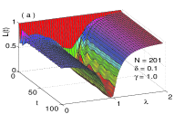
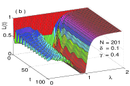
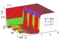
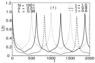
To better understand the LE (12), we plot it as a function of and in Fig.1, and as a function of only in Fig.2. For simplicity, we only set and . It is demonstrated that the decay of is enhanced at the critical point of quantum phase transition in Fig.1(a), since the XY model with corresponds to the Ising model. There exists a deep valley in the around the line , which is the same results as quan . However, for the general XY model where is adjusted in , we find that the decay of is enhanced in a different degree in the range . When , the applitudes of in Fig.1(b) is smaller than those corresponding to Fig.1(a) and the range of resulting in increases. When we continue to decrease to in Fig.1(c), it is seen that the nearly approaches zero in the range , where the central system transits from a pure state to a mixed state. So we can conclude that for a smaller , the critical point of quantum phase transition is the transition point of whether the decay of the is enhanced or not.
Comparing with the results in quan , for the general XY model, we also see that decays and revives as time increases in Fig.2(e) and (f). This may serve as a witness of QPT. At the same time, if we appropriately adjust the parameters , and as shown in Fig.2(e) and (f), it is found that the two plots of with the same have the identical profile, indicating that the period of the revival of the is proportional to the size of the surrounding system in the case of finite . Fig.2(g) and (h) reflect that the decreasing leads to fast decaying of the , which complies with the situation described by Fig.1(a)-(c). In quantum chaosperes the sensitivity of perturbations in the Hamiltonian system can be understood according to the LEjalabert . Here, for some paremeters shown in Fig.2(g) and (h), the becomes chaotic, which is due to the competition between the two phases separated by .


III Analysis of vanishing decoherence
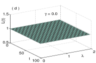
Interestingly, we find that the does not vary with time in the XX model with , i.e., the coherence of the central spin will not be affected by the special environment. The reasons are in the following. From Eqs.(6-8), we see that
| (13) |
which directly results in that the ground state of no longer lies in the two-dimensional Hilbert space spanned by and , but only one of them like Eq.(14). To obtain the explicit form of the ground state, we let and in Eq.(8), and from them know that . Considering Eqs.(8-10), we can express the ground state
| (14) |
since in Eq.(10) when , and () or (). Therefore the LE becomes
| (15) |
which means that the , initial equal to 1, will not decay at all, and the central system preserves its initial coherence except for an additional phase factor in one of eigenstate of the central system. For our model with the central system surrounded by the XX spin-1/2 bath, notice that the purity quan ; cucchietti Tr is defined to describe decoherence, it is also, independent of the central system and this special environment. What’s more, the result (15) is regardless of the number of the lattice and what the external magnetic field is, it seems to be counterintuitive, but it is indeed the case. We can see Fig.1(d). At the same time, we emphasize that the non-decay of the LE in this case is nontrivial because of the difference between and .
The result can be better understood as follows. Evolving from the initial system-environment state , which are not entangled, it becomes at an arbitrary , where and are driven by the Hamiltonians and , respectively. It is known that and are different, however, it happens that the anisotropy parameter leads to their same evolution, resulting in . The real time-dependent denotes an additional phase factor.
Finally, we assume that the XX model environment to be initially prepared in an arbitrary excited state with . A -particle state has the form , with all the distinct, i.e., it is
| (16) | |||||
where Substituting Eq.(16) into Eq.(4), we find that the LE is also, which implies that the partial excited states of the environment does not induce decoherence to the central system. However, if the environment is initially prepared in a thermal state, the LE is no longer equal to unit, but will decay with time.
Of particular interest is the case in which the XY model lies initially in an excited state. The -particle state can be written as
| (17) | |||||
After calculation by substituting Eq.(17) into Eq.(4) the LE is derived as with . It can be seen that: (i) the excited states have no any contributions to modulating the LE; (ii) if all the particles are excited, i.e., , which is assumed to be the initial state of the bath, the LE of the central system is unit also. Notice that if the initial state of the XY model bath is thermal, the LE of the central system will decay with time. The vanishing decoherence may arise in view of the non-interacting environments in cc : if we let all spins lie initially in either up or down, the decoherence factor will be unit as well. It is worthwhile for us to find out its physical nature.
IV Conclusions
In summary, for a central system uniformly coupled to a XY spin-1/2 bath in a transverse field, we explicitly calculate the Loschmidt echo(LE) to characterize decoherence quantitatively. We find that the anisotropy parameter affects decoherence of the central system sensitively when , in particular, the LE becomes unit without varying with time when , implying that environment-induced decoherence vanishes. At the same time, we show that decoherence can vanish provided that the initial state of the XX spin-1/2 bath lies in either the ground state or the partial particles are excited, or it lies in the state that all particles are excited. Although it is difficult to make the initial state of the spin bath pure at zero temperature and then difficult to fulfil the vanishing decoherence in real experiments, in a theoretical sense, our findings may shed light on understanding of decoherence.
V Acknowledgement
We greatly acknowledge the helpful discussions with H.T.Quan and X.Z.Yuan.
References
- (1) W. G .Unruh, Phys. Rev. A 51, 992 (1995).
- (2) D. P. DiVincenzo, Science 270, 225 (1995).
- (3) A. R. Calderbank and P. W. Shor 54, 1098 (1996).
- (4) A. M. Steane, Phys. Rev. Lett. 77, 793 (1996).
- (5) D. Gottesman, Stabilizer Codes and Quantum Error Correction. Ph.D. thesis, California Institute of Technology, Pasadema, CA, 1997.
- (6) D. Bacon, J. Kempe, D. A. Lidar, and K. B. Whaley, Phys. Rev. Lett. 85, 1758 (2000).
- (7) L. M. Duan and G. C. Guo, Phys. Rev. Lett. 79, 1953 (1997).
- (8) W. H. Zurek, Rev. Mod.Phys. 75, 715 (2003); Phys. Today 44, No. 10, 36(1991).
- (9) A. Peres, Quantum Theory: Concepts and Methods, (Kluwer Academic Publishers, Dordrecht, 1995).
- (10) U. Weiss, Quantum Dissipative Systems, 2nd ed. (World Scientific, Singapore, 1999).
- (11) T. J. Osborne and M. A. Nielsen, Phys. Rev. A 66, 032110 (2002).
- (12) L. A. Wu, M. S. Sarandy, and D. A. Lidar, Phys. Rev. Lett. 93, 250404 (2004).
- (13) C. M. Carollo and J. K. Pachos, Phys. Rev. Lett. 95, 157203 (2005).
- (14) S. L. Zhu, Phys. Rev. Lett. 96, 077206 (2006).
- (15) A. Hamma, quant-ph/0602091.
- (16) H. T. Quan, Z. Song, X. F. Liu, P. Zanardi, and C. P. Sun, Phys. Rev. Lett. 96, 140604 (2006).
- (17) D. Rossini, T. Calarco, V. Giovannetti, S.Montangero, R. Fazio, quant-ph/0605051.
- (18) S. Sachdev, Quantum Phase Transition (Cambridge University Press, Cambridge, 2000).
- (19) F. M. Cucchitti, D. A. R. Dalvit, J. P. Paz, and W. H. Zurek, Phys. Rev. Lett. 91, 210403(2003).
- (20) F. M. Cucchitti, J. P. Paz, and W. H. Zurek, Phys. Rev. A 72, 052113(2005).
- (21) F. M. Cucchitti, S. F. Vidal, and J. P. Paz, quant-ph/0604136.
- (22) R. A. Jalabert and H.M. Pastawski, Phys. Rev. Lett. 86, 2490 (2001).