Majorization in Quantum Adiabatic Algorithms

Abstract

The majorization theory has been applied to analyze the mathematical structure of quantum algorithms. An empirical conclusion by numerical simulations obtained in the previous literature indicates that step-by-step majorization seems to appear universally in quantum adiabatic algorithms. In this paper, a rigorous analysis of the majorization arrow in a special class of quantum adiabatic algorithms is carried out. In particular, we prove that for any adiabatic algorithm of this class, step-by-step majorization of the ground state holds exactly. For the actual state, we show that step-by-step majorization holds approximately, and furthermore that the longer the running time of the algorithm, the better the approximation.

I INTRODUCTION

In the past two decades, quantum computation has attracted a great deal of attention, for it was demonstrated that the performance of quantum algorithms exceeds that of all known classical corresponding algorithms for some computational tasks. Among all quantum algorithms proposed so far, Shor’s factorization algorithm SHOR94 and Grover’s search algorithm GROVER97 are two famous examples. However, the design of quantum algorithms seems to be very difficult Shor03 . Therefore, uncovering some underlying mathematical structure of quantum algorithms becomes a very important question. For example, it has been observed that majorization theory seems to play an important role in the efficiency of quantum algorithms OLM021 ; OLM022 ; LM02 . The intuition is that in many quantum algorithms, the initial state of the system is an equal superposition state and the final state before measurement is some computational basis state corresponding to the final result. In the process of computation, the probability distribution associated to the state of the system in the computational basis is step-by-step majorized until it is maximally ordered. In OLM021 , by carrying out a systematic analysis of a wide variety of quantum algorithms from the majorization theory point of view, R. Orús et al. concluded that step-by-step majorization is found in the known instances of fast and efficient algorithms, such as quantum fourier transform, Grover’s algorithm, the algorithm for the hidden affine function problem. On the other hand, R. Orús et al. offered an example to show that some quantum algorithms, which do not give any computational speed-up, violates step-by-step majorization. These facts indicate that step-by-step majorization seems to be necessary for the efficiency of quantum algorithms.

In OLM021 and LM02 , the analysis of the role of majorization in quantum adiabatic algorithms, a novel paradigm for the design of quantum algorithms, was also carried out. Through numerical simulations to several special cases R. Orús et al. got an empirical conclusion that quantum algorithms based on adiabatic evolution naturally show step-by-step majorization provided that the Hamiltonians and the initial state are chosen with sufficient symmetry and the evolution is slow enough.

In a quantum adiabatic algorithm, the evolution of the quantum register is governed by a hamiltonian that varies continuously and slowly. If the initial state of the system is the ground state of the initial hamiltonian, the state of the system at any moment in the whole process of computation will differ from the ground state of the hamiltonian at that moment by a negligible amount. Thus, in a quantum adiabatic algorithm the ground state of the hamiltonian is a “guide”, and the actual state of the system always evolves around this guide. In this paper, we will analyze the majorization arrow in a special class of quantum adiabatic algorithms. We prove that in any algorithm of this class step-by-step majorization of the ground state holds perfectly. For the actual state, we show that step-by-step majorization holds approximately and that the longer the running time, the better the approximation. Thus the results obtained in this paper offers stronger evidences to support the conclusion drawn by R. Orús et al.

The rest of the paper is organized as follows. In Sec. II we briefly review quantum adiabatic computation and majorization theory. In Sec. III we prove that step-by-step majorization of the ground state holds. In Sec. IV we discuss step-by-step majorization of the actual state. Finally, in Sec. V we summarize our conclusions and discuss the role majorization plays in the efficiency of quantum algorithms.

II PRELIMINARIES

For the convenience of the readers, in this section we will recall quantum adiabatic computation and majorization theory.

Quantum adiabatic computation, proposed by Farhi FGGS00 , is based on quantum adiabatic evolution. Suppose the state of a quantum system is $|\psi(t)\rangle(0\leq t\leq T)$, which evolves according to the Schrödinger equation

$$i\frac{d}{dt}|\psi(t)\rangle=H(t)|\psi(t)\rangle,$$ (1)

where $H(t)$ is the Hamiltonian of the system. Suppose $H_{0}=H(0)$ and $H_{1}=H(T)$ are the initial and the final Hamiltonians of the system. Then we let the hamiltonian of the system vary from $H_{0}$ to $H_{1}$ slowly along some path. For example, an interpolation path is one choice,

$$H(t)=f(t)H_{0}+g(t)H_{1},$$ (2)

where $f(t)$ and $g(t)$ are continuous functions with $f(0)=g(T)=1$ and $f(T)=g(0)=0$ ($T$ is the running time of the evolution). Let $|E_{0},t\rangle$ and $|E_{1},t\rangle$ be the ground state and the first excited state of the Hamiltonian at time t, and let $E_{0}(t)$ and $E_{1}(t)$ be the corresponding eigenvalues. The quantum adiabatic theorem LIS55 shows that we have

$$|\langle E_{0},T|\psi(T)\rangle|^{2}\geq 1-\varepsilon^{2},$$ (3)

provided that

$$\frac{D_{max}}{g_{min}^{2}}\leq\varepsilon,\ \ \ \ 0<\varepsilon\ll 1,$$ (4)

where $g_{min}$ is the minimum gap between $E_{0}(t)$ and $E_{1}(t)$

$$g_{min}=\min_{0\leq t\leq T}[E_{1}(t)-E_{0}(t)],$$ (5)

and $D_{max}$ is a measurement of the evolving rate of the Hamiltonian

$$D_{max}=\max_{0\leq t\leq T}|\langle E_{1},t|\frac{dH}{dt}|E_{0},t\rangle|.$$ (6)

Quantum adiabatic computation is a novel paradigm for the design of quantum algorithms. For example, Quantum search algorithm proposed by Grover GROVER97 has been implemented by quantum adiabatic computation in RC02 . Recently, the new paradigm for quantum computation has been used to try to solve some other interesting and important problems, such as Deutsch-Jozsa problem DKK02 ; SL05 ; WY06 , hidden subgroup problem RAO03 , 3SAT problem FGGS00 ; ZH06 , traveling salesman problem TDK06 and Hilbert’s tenth problem TDK01 .

Let’s first define a special class of quantum adiabatic algorithms, on which we will focus in this work. Suppose $f:\{0,1\}^{n}\rightarrow R$ is a function bounded by a polynomial of n. Let $H_{0}$ and $H_{1}$ be the initial and the final hamiltonians of a quantum adiabatic evolution with a linear path $H(t)$. Concretely,

$$H_{0}=I-|\alpha\rangle\langle\alpha|,$$ (7)

$$H_{1}=\sum\limits_{i=1}^{N}{f(i)|i\rangle\langle i|},$$ (8)

$$H(s)=(1-s)H_{0}+sH_{1},$$ (9)

where

$$|\alpha\rangle=\frac{1}{\sqrt{N}}\sum\limits_{i=1}^{N}{|i\rangle},\ \ N=2^{n},$$ (10)

and $s=s(t)$ a continuous increasing function with $s(0)=0$ and $s(T)=1$ ($T$ is the running time of the quantum adiabatic evolution). According to quantum adiabatic theorem, this class of algorithms can be used to minimize the function $f(i),i=1,2,...,N$. The quantum adiabatic algorithms for search problem in RC02 , hidden subgroup problem in RAO03 , 3SAT problem in ZH06 and traveling salesman problem in TDK06 belong to this class.

Now let’s turn to the majorization theory. Majorization is an ordering on N-dimensional real vectors. Suppose $x=(x_{1},x_{2},...,x_{N})$ and $y=(y_{1},y_{2},...,y_{N})$ are two N-dimensional vectors. If $x$ is majorized by $y$, $x$ is more disordered than another. To be concrete, let $x^{\downarrow}$ mean $x$ re-ordered so the components are in decreasing order. We say $x$ is majorized by $y$, namely $x\prec y$, provided $\sum\limits_{i=1}^{k}{x_{i}^{\downarrow}}\leq\sum\limits_{i=1}^{k}{y_{i}^{\downarrow}}$ for $k=1,2,...,N-1$ and $\sum\limits_{i=1}^{N}{x_{i}^{\downarrow}}=\sum\limits_{i=1}^{N}{y_{i}^{\downarrow}}$. It has been proven that majorization is at the heart of the solution of a large number of quantum information problems. For example, majorization characterizes when one quantum bipartite pure states can be transformed to another deterministically via local operations and classical communication Nilsen99 . For more details about majorization, see RB97 .

In OLM021 and LM02 , majorization theory was related to quantum algorithms. It can be shown as follows: let $|\psi^{(m)}\rangle$ be the state of the register of a quantum computers at an operating stage labeled by $m=1,...M$, where $M$ is the total number of steps in the algorithm. Let $N$ be the dimension of the Hilbert space. Suppose $\{|i\rangle\}_{i=1}^{N}$ is the basis in which the final measurement is performed. Then suppose in this basis the state $|\psi^{(m)}\rangle$ is

$$|\psi^{(m)}\rangle=\sum\limits_{i=1}^{N}{a_{i}^{(m)}|i\rangle}.$$ (11)

If we measure $|\psi^{(m)}\rangle$ in the basis $\{|i\rangle\}_{i=1}^{N}$, the probability distribution associated to this state is $p^{(m)}=\{p_{i}^{(m)}\}$, where

$$p_{i}^{(m)}\equiv|a_{i}^{(m)}|^{2}=|\langle i|\psi^{(m)}\rangle|^{2},\ \ i=1,2,...,N.$$ (12)

If $p^{(m)}\prec p^{(m+1)}$ for every $m$, we say this algorithm enjoys the majorization relation step by step.

Especially, majorization theory has been applied to analyze quantum adiabatic algorithms. Suppose $t_{1}$ and $t_{2}$ are two arbitrary time point in an adiabatic evolution, and $t_{1}<t_{2}$. If it always holds that the probability distribution associated to the state of the system at $t_{1}$ is majorized by that at $t_{2}$, we say this adiabatic algorithm enjoys step-by-step majorization. In OLM021 and LM02 , R. Orús et al. studied majorization in local and global quantum adiabatic search algorithms. Note that both these two algorithms belong to the class of quantum adiabatic algorithms we will discuss.

III STEP-BY-STEP MAJORIZATION OF THE GROUND STATE

As mentioned above, in a quantum adiabatic algorithm, the state of the system at any time is always close to the ground state of the hamiltonian of that moment with a small distance. So analyzing the evolution of the ground state may help us to understand that of the actual state.

In this section, we prove that, for any quantum adiabatic algorithm of the class of quantum adiabatic algorithms described by Eqs.(7)-(10), step-by-step majorization of the ground state holds perfectly. Before proving this result, we first consider the following two lemmas.

We have known that the purpose of quantum adiabatic algorithms given by Eqs.(7)-(10) is to find the minimum of the function $f(x)$. The following lemma shows that only the range of $f(x)$ affects our discussion and the distribution of this set does not.

Lemma 1

Suppose there are two quantum adiabatic evolutions given by Eqs.(7)-(10) with different $H_{1}$. Concretely, these two final hamiltonians are

$$H_{1}=\sum\limits_{i=1}^{N}{f(i)|i\rangle\langle i|}$$ (13)

and

$$H_{1}^{\prime}=\sum\limits_{i=1}^{N}{f^{\prime}(i)|i\rangle\langle i|},$$ (14)

where $f^{\prime}(i)=f(\pi(i))$. Here $\pi$ is a permutation of $1,2,...,N$. Let the ground states of these two quantum adiabatic evolution be real vectors $(a_{1},a_{2},...,a_{N})^{T}$ and $(a_{1}^{\prime},a_{2}^{\prime},...,a_{N}^{\prime})^{T}$, respectively. Then we have

$$a_{i}^{\prime}=a_{\pi(i)},1\leq i\leq N.$$ (15)

Proof. The proof is easy as long as we note that $P_{\pi}H^{\prime}(s)P_{\pi}=H(s)$, where $P_{\pi}$ is a permutation matrix such that $P_{\pi}|i\rangle=|\pi(i)\rangle$ and

$$H^{\prime}(s)=(1-s)H_{0}+sH_{1}^{\prime}.$$ (16)

$\Box$

It can be shown that we can choose the global phase of the ground state of $H(s)$ given by Eq.(9) such that it is a real vector. In this paper, we always assume ground states to be real.

Usually, it is difficult to work out the ground state of $H(s)$ exactly. However, the following lemma indicates that there are close relations among the components of this ground state. Our proof for the main result of this section is based on these relations.

Lemma 2

Suppose there is a quantum adiabatic evolutions given by Eqs.(7)-(10). Let real vector

$$|\psi(s)\rangle=(a_{1},a_{2},...,a_{N})^{T}$$ (17)

be the ground state of this quantum adiabatic evolution and $\lambda(s)$ the corresponding eigenvalue. Then we have

$$(t(s)+sf(i))a_{i}=(t(s)+sf(j))a_{j},\ \ i,j=1,2,...,N,$$ (18)

where $t(s)=1-s-\lambda(s)$ is a strictly decreasing function of $s$.

Proof. By the definitions of $|\psi(s)\rangle$ and $\lambda(s)$, we have

$$H(s)|\psi(s)\rangle=\lambda(s)|\psi(s)\rangle.$$ (19)

Substituting Eq.(9) and Eq.(17) into Eq.(19) yields

$$\frac{1-s}{N}\sum_{i=1}^{N}{a_{i}}=t(s)a_{i}+sf(i)a_{i},$$ (20)

where $t(s)=1-s-\lambda(s)$. Note that $t(s)$ is the biggest eigenvalue of

$$G(s)=(1-s)I-H(s).$$ (21)

For every $s\in[0,1)$ and $ds>0$, an explicit calculation shows that

$$G(s+ds)-G(s)=-ds\times(|\alpha\rangle\langle\alpha|+\sum\limits_{i=1}^{N}{f(i)|i\rangle\langle i|}).$$ (22)

Because $G(s)-G(s+ds)$ is a strictly positive matrix, it can be shown that $t(s)$ is a strictly decreasing function of $s$ RB97 . It is easy to get $t(0)=1$ and $t(1)=0$. Then we have $0<t(s)<1$ for any $s\in(0,1)$.

By Eq.(20) we can obtain

$$(t(s)+sf(i))a_{i}=(t(s)+sf(j))a_{j},\ \ i,j=1,2,...,N.$$ (23)

$\Box$

Now we are able to present the main result of this section. It establishes the step-by-step majorization property of the ground state of $H(s)$.

Theorem 1

Suppose $H_{0}$ and $H_{1}$ given by Eq.(7) and Eq.(8) are the initial and the final hamiltonians of a quantum adiabatic algorithm. Suppose this quantum adiabatic algorithm has a linear path given by Eq.(9). Then the ground state of this algorithm shows perfect step-by-step majorization.

Proof. Suppose the ground state of $H(s)$ is

$$|\psi(s)\rangle=(a_{1},a_{2},...,a_{N})^{T},$$ (24)

and the corresponding eigenvalue is $\lambda(s)$. Suppose $\min_{1\leq i\leq N}f(i)=0$. Otherwise we can let

$$H(s)=H(s)-s\times I\times\min_{1\leq i\leq N}f(i),$$ (25)

which doesn’t change the ground state of $H(s)$. For convenience we suppose $f(1)\leq f(2)\leq f(3)\leq...\leq f(N)$, which doesn’t affect our analysis for majorization later by Lemma 1. On the other hand, by Lemma 2 we have

$$(t(s)+sf(i))a_{i}=(t(s)+sf(j))a_{j},\ \ i,j=1,2,...,N,$$ (26)

where $t(s)$ is defined as before. Substituting Eq.(26) into

$$\sum_{i=1}^{N}{{a_{i}}^{2}}=1$$ (27)

gives

$${a_{1}}^{2}=\frac{1}{\sum_{i=1}^{N}{(\frac{1}{1+\frac{s}{t(s)}f(i)})^{2}}}.$$ (28)

Note that $t(s)$ is a strictly decreasing function of $s$, which means $a_{1}$ is a strictly increasing function of $s$. For any other $a_{i}$, the monotony is a little more complicated. It’s possible that they are not monotonous. However, we can prove that their increasing and decreasing are well-regulated. Concretely, for $s>0$ and $1-s\geq ds>0$, let $({a_{1}}^{\prime},{a_{2}}^{\prime},...,{a_{N}}^{\prime})^{T}$ be the ground state of $H(s+ds)$. Then we have if $a_{i}\geq{a_{i}}^{\prime}$, $a_{j}\geq{a_{j}}^{\prime}$, where $i<j$.

This conclusion can be proved as follows. From Eq.(26), we obtain

$$\frac{a_{i}}{a_{j}}=\frac{t(s)+sf(j)}{t(s)+sf(i)},$$ (29)

and

$$\frac{{a_{i}}^{\prime}}{{a_{j}}^{\prime}}=\frac{t(s+ds)+(s+ds)f(j)}{t(s+ds)+(s+ds)f(i)}.$$ (30)

Because $t(s)$ is a strictly decreasing function, it can be checked that

$$\frac{t(s)+sf(j)}{t(s)+sf(i)}\leq\frac{t(s+ds)+(s+ds)f(j)}{t(s+ds)+(s+ds)f(i)}.$$ (31)

So,

$$\frac{a_{i}}{a_{j}}\leq\frac{{a_{i}}^{\prime}}{{a_{j}}^{\prime}}.$$ (32)

Thus if ${a_{i}}^{\prime}\leq a_{i}$, we have ${a_{j}}^{\prime}\leq a_{j}$.

According to the discussion above, we know that for every $s\in(0,1)$ there is a special integer $i_{0}(s)$. When $i\leq i_{0}(s)$ we have $a_{i}\leq{a_{i}}^{\prime}$ and when $i>i_{0}(s)$ we have $a_{i}>{a_{i}}^{\prime}$.

Now we are in a position to prove our main conclusion. Namely,

$$({a_{1}}^{2},{a_{2}}^{2},...,{a_{N}}^{2})^{T}\prec({a_{1}}^{\prime 2},{a_{2}}^{\prime 2},...,{a_{N}}^{\prime 2})^{T}.$$ (33)

Firstly, according to Eq.(26) it can be checked that the components of $({a_{1}}^{2},{a_{2}}^{2},...,{a_{N}}^{2})^{T}$ and $({a_{1}}^{\prime 2},{a_{2}}^{\prime 2},...,{a_{N}}^{\prime 2})^{T}$ are in decreasing order. Secondly, for any $s\in(0,1)$ and any $k=1,2,...,N$, if $k\leq i_{0}(s)$, we have $\sum\limits_{i=1}^{k}{a_{i}^{2}}\leq\sum\limits_{i=1}^{k}{a_{i}^{\prime 2}}$ because $a_{i}\leq a_{i}^{\prime}$ for $i\leq k$. If $k>i_{0}(s)$, $a_{i}>a_{i}^{\prime}$ for $i\geq k$, so we have $\sum\limits_{i=k+1}^{N}{a_{i}^{2}}\geq\sum\limits_{i=k+1}^{N}{a_{i}^{\prime 2}}$. Thus we also get $\sum\limits_{i=1}^{k}{a_{i}^{2}}\leq\sum\limits_{i=1}^{k}{a_{i}^{\prime 2}}$ because $\sum\limits_{i=1}^{N}{a_{i}^{2}}=\sum\limits_{i=1}^{N}{a_{i}^{\prime 2}}=1$. This completes the proof of Eq.(33). Namely, step-by-step majorization of the guide state holds perfectly. $\Box$

Note that if the form of Eq.(7) doesn’t change, we can replace the ground state $|\alpha\rangle$ in Eq.(7) with any other vector of Hadamard basis and get the same conclusion. Because it can be proved if $|\alpha\rangle$ is replaced by any other vector of Hadamard basis, for any $s$ any component of the ground state of $H(s)$ will not change up to the sign. Moreover, it can be shown that the path in Eq.(9) along which the hamiltonian varies can also be replaced by any interpolation path in Eq.(2) provided $\frac{g(t)}{f(t)+g(t)}$ is a increasing function of $t$, which doesn’t destroy step-by-step majorization either.

IV STEP-BY-STEP MAJORIZATION OF THE ACTUAL STATE

In this section, based on the result of the above section we consider the majorization relation in the actual state of quantum adiabatic algorithms of the class discussed in this paper. We show that step-by-step majorization of the actual state holds approximately, and the degree of the approximation is determined by the running time OLM021 ; LM02 .

Suppose in a quantum adiabatic evolutions given by Eqs.(7)-(10), the actual state of the system is

$$|\psi^{\prime}(s)\rangle=(b_{1},b_{2},...,b_{N})^{T}.$$ (34)

Let

$$B_{k}=\sum_{i=1}^{k}{|b_{i}|^{2}},\ \ k=1,2,...,N.$$ (35)

In OLM021 R. Orús et al. studied $s-B_{1}$ curve ($B_{1}$ is the probability of finding the right solution) and $s-B_{2}$ curve of global quantum adiabatic evolution for search problem by numerical simulations. If step-by-step majorization holds perfectly, these curves should be monotonous. However, they observed that oscillation appears at the end of $s-B_{1}$ curve and $s-B_{2}$ curve, which destroys step-by-step majorization (See Figure.1). Furthermore, they also observed that the oscillation becomes weaker and weaker and step-by-step majorization tends to appear as long as the running time becomes longer and longer.

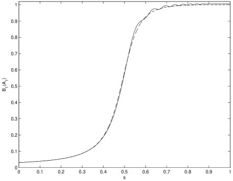
Figure 1: A case that oscillation appears at the end of $s-B_{1}$ curve (the solid curve). The dashed curve is $s-A_{1}$ curve.

Now, we prove that for any quantum adiabatic evolution of the class discussed in this paper, the oscillation at the end of $s-B_{k}(1\leq k\leq N)$ curve, if any, will continue decreasing in amplitude if the running time becomes longer and longer.

We consider an arbitrary state of the system near the end of the quantum adiabatic evolution. Let

$$A_{k}=\sum_{i=1}^{k}{a_{i}^{2}},\ \ k=1,2,...,N,$$ (36)

where $(a_{1},a_{2},...,a_{N})^{T}$ is the ground state as before. Then from Eq.(26) and Eq.(28) we have

$$A_{k}=\frac{\sum_{i=1}^{k}{(\frac{1}{1+\frac{s}{t}f(i)})^{2}}}{\sum_{i=1}^{N}{(\frac{1}{1+\frac{s}{t}f(i)})^{2}}},\ \ k=1,2,...,N,$$ (37)

From Eq.(9) it holds that

$$\frac{H(s)}{1-s}=H_{0}+\frac{s}{1-s}H_{1}\ (s<1).$$ (38)

It can be seen that $\frac{\lambda(s)}{1-s}$, the ground state eigenvalue of $\frac{H(s)}{1-s}$, is a strictly increasing function of $s$ RB97 . So

$$\frac{d}{ds}(\frac{\lambda}{1-s})>0,$$ (39)

which makes

$$\frac{d}{ds}(\frac{t}{1-s})=\frac{d}{ds}(\frac{1-s-\lambda}{1-s})<0.$$ (40)

A simple calculation shows that

$$-\frac{dt}{ds}>\frac{t}{1-s},$$ (41)

then

$$\frac{d}{ds}(\frac{s}{t})>\frac{s}{t}(\frac{1}{s}+\frac{1}{1-s}),\ \ 0<s<1.$$ (42)

Calculating the derivative of Eq.(37) we obtain

$$\frac{dA_{k}}{ds}= 2\sum_{i=2}^{k}\sum_{j=k+1}^{N}{a_{i}^{2}a_{j}^{2}(\frac{f(j)\frac{d}{ds}(\frac{s}{t})}{1+\frac{s}{t}f(j)}-\frac{f(i)\frac{d}{ds}(\frac{s}{t})}{1+\frac{s}{t}f(i)})}$$ (43)

$$+2a_{1}^{2}\sum_{i=k+1}^{N}{a_{i}^{2}\frac{f(i)\frac{d}{ds}(\frac{s}{t})}{1+\frac{s}{t}f(i)}}.$$ (44)

Since

$$\frac{f(j)\frac{d}{ds}(\frac{s}{t})}{1+\frac{s}{t}f(j)}>\frac{f(i)\frac{d}{ds}(\frac{s}{t})}{1+\frac{s}{t}f(i)}$$ (45)

when $N\geq j>i\geq 1$, we have

$$\frac{dA_{k}}{ds}>2a_{1}^{2}\sum_{i=k+1}^{N}{a_{i}^{2}\frac{f(i)\frac{d}{ds}(\frac{s}{t})}{1+\frac{s}{t}f(i)}}.$$ (46)

Let $m=\min_{2\leq i\leq N}f(i)$. If $m>1$, it holds that

$$\begin{aligned} \frac{f(i)\frac{d}{ds}(\frac{s}{t})}{1+\frac{s}{t}f(i)}>&\frac{\frac{s}{t}f(i)(\frac{1}{s}+\frac{1}{1-s})}{\frac{s}{t}f(i)+1}\\ >&\frac{\frac{f(i)}{t}+\frac{s}{t}f(i)}{1+\frac{s}{t}f(i)}\\ >&1.\end{aligned}$$ (47)

Here, we use Eq.(42) and the fact $t<1<f(i)$ and $\frac{1}{1-s}>1$. Similarly, if $m<1$, it follows that

$$\begin{aligned} \frac{f(i)\frac{d}{ds}(\frac{s}{t})}{1+\frac{s}{t}f(i)}>&\frac{\frac{s}{t}f(i)(\frac{1}{s}+\frac{1}{1-s})}{\frac{s}{t}f(i)+1}\\ =&m\frac{\frac{1}{m}\cdot\frac{f(i)}{t}+\frac{1}{m(1-s)}\frac{s}{t}f(i)}{1+\frac{s}{t}f(i)}\\ >&m.\end{aligned}$$ (48)

Thus we obtain

$$\frac{f(i)\frac{d}{ds}(\frac{s}{t})}{1+\frac{s}{t}f(i)}>c,$$ (49)

where $c=min\{m,1\}$. Substituting Eq.(48) into Eq.(45), we have

$$\frac{dA_{k}}{ds}>2c\cdot a_{1}^{2}\sum_{i=k+1}^{N}{a_{i}^{2}}.$$ (50)

Note that

$$a_{1}^{2}>\frac{\sum_{i=1}^{k}{a_{i}^{2}}}{k}=\frac{1}{k}A_{k}.$$ (51)

We finally obtain

$$\frac{dA_{k}}{ds}>\frac{2c}{k}A_{k}(1-A_{k}).$$ (52)

According to quantum adiabatic theorem, we know that for any positive $\delta$ we have a finite running time $T$ such that

$$|\langle\psi^{\prime}(s)|\psi(s)\rangle|\geq 1-\delta^{2}/2$$ (53)

for any $s\in(0,1)$. Since

$$\begin{aligned} ||\psi\rangle-|\psi^{\prime}\rangle|^{2}=&2-2\langle\psi(s)|\psi^{\prime}(s)\rangle\\ <&\delta^{2},\end{aligned}$$ (54)

it can be seen that for any $s$

$$\sum_{i=1}^{k}|a_{i}-b_{i}|^{2}<\delta^{2}.$$ (55)

Here, we choose the global phase of $|\psi^{\prime}(s)\rangle$ such that $\langle\psi(s)|\psi^{\prime}(s)\rangle$ is real. According to Cauchy’s inequality, it holds that

$$\sum_{i=1}^{k}|a_{i}-b_{i}|<\sqrt{k}\delta.$$ (56)

Note that

$$|a_{i}+b_{i}|<2,$$ (57)

it follows that

$$\sum_{i=1}^{k}|a_{i}^{2}-b_{i}^{2}|=\sum_{i=1}^{k}|a_{i}-b_{i}|\cdot|a_{i}+b_{i}|<2\sqrt{k}\delta.$$ (58)

Thus

$$|\sum_{i=1}^{k}|a_{i}|^{2}-\sum_{i=1}^{k}|b_{i}|^{2}|\leq\sum_{i=1}^{k}|a_{i}^{2}-b_{i}^{2}|<2\sqrt{k}\delta.$$ (59)

Now let us consider two points $(s_{1},A_{k}^{\prime})$ and $(s_{2},A_{k})$ on $s-A_{k}$ curve (about the ground state) and two points $(s_{1},B_{k}^{\prime})$ and $(s_{2},B_{k})$ on $s-B_{k}$ curve (about the actual state), where $s_{2}-s_{1}=\triangle s$, $0<\triangle s\ll 1$. These four points are all near the end of the quantum adiabatic evolution. If step-by-step majorization of the actual state holds, $s-B_{k}$ curve should be a monotonically increasing curve. Suppose that Eq.(52) holds. According to Eq.(58) we have

$$|A_{k}-B_{k}|<2\sqrt{k}\delta,\ \ \ |A_{k}^{\prime}-B_{k}^{\prime}|<2\sqrt{k}\delta.$$ (60)

On the other hand, according to the discussion above, it holds that

$$A_{k}-A_{k}^{\prime}>\frac{2c}{k}A_{k}(1-A_{k})\cdot\bigtriangleup s.$$ (61)

Then if

$$\delta<\frac{c}{2k\sqrt{k}}A_{k}(1-A_{k})\cdot\bigtriangleup s,$$ (62)

we have $B_{k}^{\prime}<B_{k}$.

Note that for arbitrary small $\bigtriangleup s$ we can find a corresponding $\delta$ or running time $T$ such that Eq.(61) holds. Thus, it can be judged that when the running time continues becoming longer, the oscillation at the end of $s-B_{k}$ curve becomes weaker and weaker. This explains the results of numerical simulations for global adiabatic search algorithms in OLM021 , which is a special case of our discussion above. In fact, this is consistent with our intuition. By quantum adiabatic theorem, we know that when the running time becomes longer, the distance between the actual state of the system and the ground state becomes smaller. Since it has been shown that the ground states shows exact step-by-step majorization, it’s natural that the actual state enjoys the same relation approximately. The longer the running time, the better the approximation.

It should be pointed out that this paper only deals with a special class of quantum adiabatic algorithms. Whether all quantum adiabatic algorithms enjoy step-by-step majorization (exactly or approximately) remains open.

V CONCLUSION

In conclusion, we have shown that for any algorithm of a special class of quantum adiabatic algorithms, step-by-step majorization of the ground state holds perfectly. We have also shown that step-by-step majorization of the actual state holds approximately. This supports the conclusion that majorization seems to appear universally in quantum adiabatic algorithms. For further studies, whether step-by-step majorization holds for more quantum adiabatic algorithms should be examined carefully.

As mentioned at the beginning of this paper, step-by-step majorization has been applied to analyze the efficiency of quantum algorithms by Latorre et al LM02 . They pointed out that that just obeying step-by-step majorization can not guarantee the efficiency OLM021 . The results obtained in this paper offer facts to indicate the same conclusion. It have been shown that the running time of the class of algorithms discussed in this paper is exponential in $n$, the problem size ZH06 ; FGGN05 ; RAO05 ; WY061 . It seems that the performance of these algorithms are not very good. However, these algorithms are in different situation in efficiency. Some of them are optimal, such as local adiabatic search algorithm RC02 , while the others are not, such as the adiabatic algorithm for the hidden subgroup problem RAO03 . However, as pointed out above, these algorithms enjoy the similar majorization relation. On the other hand, Latorre et al illustrated that all known fast and efficient quantum algorithms show step-by-step majorization. For further studies, whether step-by-step majorization is really necessary for efficiency is an important and interesting question.

VI ACKNOWLEDGMENTS

We are grateful to R. Orús, J. I. Latorre and M. A. Martín-Delgado for helpful comments and suggestions. We thank the colleagues in the Quantum Computation and Information Research Group for helpful discussions. This work was partly supported by the National Nature Science Foundation of China (Grant Nos. 60503001, 60321002, and 60305005).

References

- (1) Shor. P. W, Proc. 35th Annual Symposium on the Foundations of Computer Science, Shafi Goldwasser, ed., (IEEE Computer Society Press), 121-134 (1994).
- (2) L. K. Grover, Phys. Rev. Lett 79, 325 (1997); e-print quant-ph/9706033.
- (3) P. Shor, Jorurnal of the ACM, 50(1), 87-90 (2003).
- (4) R. Orús, J. I. Latorre and M. A. Martín-Delgado, European Physical Journal D 29 119 (2004); e-print quant-ph/0212094.
- (5) J. I. Latorre and M. A. Martín-Delgado, Phys. Rev. A 66 022305 (2002); e-print quant-ph/0111146.
- (6) R. Orús, J. I. Latorre and M. A. Martín-Delgado, Quantum Information Processing 1 283 (2002); e-print quant-ph/0206134.
- (7) E. Farhi, J. Goldstone, S. Gutmann, M. Sipser; e-print quant-ph/0001106.
- (8) L. I. Schiff, Quantum Mechanics (McGraw-Hill, Singapore, 1955).
- (9) J. Roland and N. J. Cerf, Phys. Rev. A 65, 042308(2002); e-print quant-ph/0107015.
- (10) S. Das, R. Kobes, G. Kunstatter, Phys. Rev. A 65, 062310(2002); e-print quant-ph/0111032.
- (11) M. S. Sarandy and D. A. Lidar, Phys. Rev. Lett 95, 250503(2005); e-print quant-ph/0502014.
- (12) Z. Wei and M. Ying, Phys. Lett. A 354, 271 (2006); e-print quant-ph/0512008.
- (13) M. V. Panduranga Rao, Phys. Rev. A 67, 052306(2003).
- (14) M.Znidaric and M. Horvat, Phys. Rev. A 73, 022329(2006); e-print quant-ph/0509162.
- (15) T. D. Kieu, e-print quant-ph/0601151.
- (16) T. D. Kieu, e-print quant-ph/0110136.
- (17) E. Farhi, J. Goldstone, S. Gutmann and D. Nagaj, e-print quant-ph/0512159.
- (18) M. V. Panduranga Rao, Technical Report IISc-CSA-TR-2005 C17, http://archive.csa.iisc.ernet.in/TR/2005/17/.
- (19) Z. Wei and M. Ying, e-print quant-ph/0604077.
- (20) M. A. Nielsen, Phys. Rev. Lett. 83, 436 (1999); e-print quant-ph/9811053.
- (21) R. Bhatia, Matrix Analysis, Springer-Verlag, 1997.