Abstract

Permutation and its partial transpose play important roles in quantum information theory. The Werner state is recognized as a rational solution of the Yang–Baxter equation, and the isotropic state with an adjustable parameter is found to form a braid representation. The set of permutation’s partial transposes is an algebra called the “PPT” algebra which guides the construction of multipartite symmetric states. The virtual knot theory having permutation as a virtual crossing provides a topological language describing quantum computation having permutation as a swap gate. In this paper, permutation’s partial transpose is identified with an idempotent of the Temperley–Lieb algebra. The algebra generated by permutation and its partial transpose is found to be the Brauer algebra. The linear combinations of identity, permutation and its partial transpose can form various projectors describing tangles; braid representations; virtual braid representations underlying common solutions of the braid relation and Yang–Baxter equations; and virtual Temperley–Lieb algebra which is articulated from the graphical viewpoint. They lead to our drawing a picture called the “ABPK” diagram describing knot theory in terms of its corresponding algebra, braid group and polynomial invariant. The paper also identifies nontrivial unitary braid representations with universal quantum gates, and derives a Hamiltonian to determine the evolution of a universal quantum gate, and further computes the Markov trace in terms of a universal quantum gate for a link invariant to detect linking numbers.

Key Words: Partial Transpose, Temperley–Lieb Algebra, Virtual Braid

PACS numbers: 02.10.Kn, 03.65.Ud, 03.67.Lx

1 Introduction

In a vector space $V$, there are rich algebraic structures over the direct sum of its tensor products $V^{\otimes n},n\in{\mathbb{N}}$, for example, the braid relation describing knot theory [1]. In the vector space $V^{\otimes n}$, two types of operations can be defined: either global or local. For example, the transpose in $V^{\otimes n}$ is a global operator on $V^{\otimes n}$ itself, while the partial transpose is a local operator in $V^{\otimes n}$ and acts on the subspace of $V^{\otimes n}$. The paper focuses on the permutation $P$ and its partial transpose $P_{\ast}$ and tries to exhaust their underlying algebraic and topological properties.

The paper’s goals take root in quantum information theory [2]. The partial transpose itself has become a standard tool in quantum entanglement theories for detecting the separability of a given quantum state, see [3] for more references. The Peres–Horodecki criterion [4, 5] says that the partial transpose of a separable density operator is positive. A state $\rho$ is called separable or “classically correlated”, i.e., convex combinations of product density operators [6, 7],

$$\rho=\sum_{i}\lambda_{i}\,\rho_{A}^{(i)}\otimes\rho_{B}^{(i)},\,\,\Theta_{2}(\rho)=\sum_{i}\lambda_{i}\,\rho_{A}^{(i)}\otimes\Theta(\rho_{B}^{(i)}),\,\,\sum_{i}\lambda_{i}=1,\,\,\lambda_{i}\geq 0$$ (1)

where the symbol $\Theta_{2}$ denotes the partial transpose, the symbol $\Theta$ denotes the transpose and $\rho_{A}$, $\rho_{B}$ are states for subsystems $A$, $B$, respectively.

Here the Werner state [7] is identified as a rational solution of the Yang–Baxter equation (YBE) [8, 9], i.e., $Id+uP$ as the linear combination of identity and permutation, while the isotropic state [10] is found to form a braid representation, i.e., $Id+vP_{\ast}$ with a specified parameter $v$. Permutation as an element of the group algebra ${\cal S}_{n}$ of the symmetric group $S_{n}$ and its partial transpose form a new algebra called the $PPT_{n}$ algebra which is isomorphic to the Brauer algebra [11]. It plays important roles in constructing multipartite symmetric states [12, 13] in quantum information theory. In terms of Brauer diagrams, complicated computations can be simplified, for example, proving that quantum data hiding is at least asymptotically secure in the large system dimension [13, 14].

Recently, knot theory is involved in the study of quantum information theory. A series of papers explore natural similarities between topological entanglement and quantum entanglement, see [15, 16, 17] for universal quantum gates and unitary solutions of the YBE; see [18, 19, 20] for quantum topology and quantum computation; see [21, 22] for quantum entanglement and topological entanglement; see [23] for teleportation topology. They identify nontrivial unitary solutions of the YBE with universal quantum gates.

Now let $P$ be a swap permutation matrix specified by $P(|\xi\rangle\otimes|\eta\rangle)=|\eta\rangle\otimes|\xi\rangle$ and let the $\check{R}$-matrix be a unitary solution to the braid relation (the braid version of the YBE). Examples are the following forms

$$\check{R}=\left(\begin{array}[]{cccc}a&0&0&0\\ 0&0&d&0\\ 0&c&0&0\\ 0&0&0&b\end{array}\right),\qquad\tau=\check{R}P=\left(\begin{array}[]{cccc}a&0&0&0\\ 0&c&0&0\\ 0&0&d&0\\ 0&0&0&b\end{array}\right),$$ (2)

where $a,b,c,d$ can be any scalars on the unit circle in the complex plane. From the point of view of braiding and algebra, $\tau$ is a solution to the algebraists version of the YBE with $\tau=\check{R}P$, and $P$ is to be regarded as an algebraic permutation or as a representation of a virtual or flat crossing. Then from the point of view of quantum gates, we have the phase gate $\tau$ and the swap gate $P$. The $\check{R}$-matrix can be used to make an invariant of knots and links that is sensitive to linking numbers.

The virtual braid group [24, 25, 26, 27] is an extension of the classical braid group by the symmetric group. Each virtual braid operator can be interpreted as a swap gate. With virtual operators in place, we can compose them with the $\check{R}$-matrix to obtain phase gates and other apparatus in quantum computation. Therefore the virtual braid group provides a useful topological language for building patterns of quantum computing.

Besides applications of permutation and its partial transpose to quantum information theory, there are unexpected underlying algebraic and topological structures. Here the permutation’s partial transpose $P_{\ast}$ is recognized as an idempotent of the Temperley–Lieb ($TL$) algebra [28]. The projectors in terms of $Id$, $P$ and $P_{\ast}$ suggest the concept of the $D_{n}$ tangle allowing both classical and virtual crossings which generalizes the $T_{n}$ tangle only having classical crossings [29]. It is well known that braids can be represented in the $TL$ algebra [30, 31, 32]. The linear combinations of $Id$, $P$ and $P_{\ast}$ are found to form braid representations, for example the isotropic state $Id+vP_{\ast}$; flat braid representations underlying common solutions of the braid relation and YBEs; unitary braid representation via Yang–Baxterization [33] and a general unitary braid representation observed from a solution of the coloured YBE [34, 35].

In view of a series of results in this paper, we articulate the concept of the virtual Temperley–Lieb algebra which forms a virtual braid representation similar to the $TL$ algebra representation of the braid group. We define a generalized Temperley–Lieb algebra which is isomorphic to the Brauer algebra in the graphical sense. As a natural summary, we draw the ABPK diagram describing knot theory in terms of its corresponding algebra, braid and polynomial to emphasize roles of the virtual Temperley–Lieb algebra in the virtual knot theory.

The plan of our paper is organized as follows. Section 2 interprets permutation’s partial transpose as an idempotent of the $TL$ algebra and introduces the concept of the $D_{n}$ tangle. Section 3 observes the Werner state and isotropic state from the point of YBE solutions under dual symmetries. Section 4 defines the $PPT_{n}$ algebra and lists the axioms of the Brauer algebra with an example generated by the permutation $P^{\pm}$ and its partial transpose’s deformation $Q_{\ast}$. Section 5 presents the family of virtual braid groups by sketching axioms defining virtual, welded and unrestricted braid groups. Section 6 applies the linear combinations of $Id$, $P$ and $P_{\ast}$ to virtual braid representations and YBE solutions, and proposes the virtual Temperley–Lieb algebra and show it in the $ABPK$ diagram. Section 7 identifies nontrivial unitary braid representations with universal quantum gates and calculates the Markov trace for a link invariant to support such an identification. The last section concludes the paper and makes comments on further research. The appendix A sketches the Hecke algebra representation of the braid group. The appendix B provides a proof for Theorem 1.

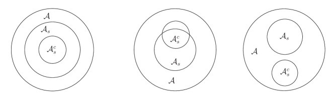
Figure 1: The commutant ${\cal A}^{c}_{s}$ of the subalgebra ${\cal A}_{s}$ of the algebra $\cal A$.

The braid representation $\sigma$-matrix and YBE solution $\check{R}$-matrix are $d^{2}\times d^{2}$ matrices acting on $V\otimes V$ where $V$ is an $d$-dimensional complex vector space. The $\sigma$-matrix ($\check{R}$-matrix) is essentially a generalization of permutation [8, 9]. The symbols $\sigma_{i}$ and $\check{R}_{i}$ denote $\sigma$ and $\check{R}$ acting on the tensor product $V_{i}\otimes V_{i+1}$. The symbols $Id$ or $1\!\!1$ denote the identity map from $V$ to $V$. The commutant of the algebra ${\cal A}_{s}$, a subalgebra of the algebra ${\cal A}$, is the set ${\cal A}_{s}^{c}$ of elements of the algebra ${\cal A}$ commuting with all elements of the subalgebra ${\cal A}_{s}$, so that it is either a subset or independent of ${\cal A}_{s}$ or intersects ${\cal A}_{s}$, see Figure 1.

2 Permutation and its partial transpose

We define the permutation $P$, and realize its partial transpose $P_{\ast}$ to be an idempotent of the $TL$ algebra. We combine $Id$, $P$ and $P_{\ast}$ into projectors, propose the concept of the $D_{n}$ tangle and finally make diagrammatic representations for the extended Temperley–Lieb algebra.

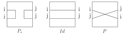
Figure 2: Permutation, permutation’s partial transpose and identity.

2.1 Permutation’s partial transpose

For two given independent finite Hilbert spaces ${\cal H}_{1}$ and ${\cal H}_{2}$ with bases $\{|i\rangle\}$ and $\{|j\rangle\}$ respectively, the tensor products $|i\rangle\otimes|j\rangle$ denoted by $|ij\rangle$, $i,j=1,\cdots,d$, gives the product basis for ${\cal H}_{1}\otimes{\cal H}_{2}$. The permutation operator $P$ has the form as $P=\sum_{i,j=1}^{d}|ij\rangle\langle ji|$ which satisfies $P|\xi\eta\rangle=|\eta\xi\rangle$. See Figure 2. The partial transpose operator $\Theta_{2}$ is defined by acting on the operator product $A\otimes B$ and only transforming indices belonging to the basis of the second Hilbert space ${\cal H}_{2}$, namely $\Theta_{2}(A\otimes B)=A\otimes B^{T}$. When the basis of ${\cal H}_{2}$ is fixed, the symbol $B^{T}$ denotes the transpose of the matrix $B$. With the partial transpose $\Theta_{2}$ acting on the permutation $P$, we have a new operator $P_{\ast}$ given by

$$P_{\ast}=\Theta_{2}\circ P=\sum^{d}_{i,j=1}(|i\rangle\otimes\langle j|)(|j\rangle\otimes\langle i|)^{T}=d|\Omega\rangle\langle\Omega|,\qquad|\Omega\rangle=\frac{1}{\sqrt{d}}\sum_{i=1}^{d}|ii\rangle$$ (3)

where $|\Omega\rangle$ is called the Schmidt form and $P_{\ast}$ acts on $|\xi\eta\rangle$ by

$$P_{\ast}|\xi\eta\rangle=\sum_{i,j=1}^{d}|ii\rangle\langle jj|\xi\eta\rangle=\sum_{i=1}^{d}|ii\rangle\delta_{\xi\eta}.$$ (4)

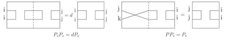
Figure 3: The products of $P_{\ast}$ and $P$, $P_{\ast}$.

The permutation $P$ and its partial transpose $P_{\ast}$ satisfy $PP_{\ast}=P_{\ast}P=P_{\ast}$ and $P_{\ast}P_{\ast}=d\,P_{\ast}$, see Figure 3. In the four dimensional case (d=2), the operators $P$ and $P_{\ast}$ have the forms in matrix:

$$P=\left(\begin{array}[]{cccc}1&0&0&0\\ 0&0&1&0\\ 0&1&0&0\\ 0&0&0&1\end{array}\right),\qquad P_{\ast}=\left(\begin{array}[]{cccc}1&0&0&1\\ 0&0&0&0\\ 0&0&0&0\\ 1&0&0&1\end{array}\right).$$ (5)

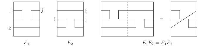
Figure 4: The generators $E_{1}$ and $E_{2}$ of the $TL_{3}$ algebra.

The permutation’s partial transpose $P_{\ast}$ is an idempotent of the $TL$ algebra. The $TL_{n}(\chi)$ algebra is generated by $1\!\!1$ and $n-1$ hermitian operators $E_{i}$ satisfying

$$TLR(\chi):\,\,E_{i}^{2} = \chi E_{i},\qquad(E_{i})^{\dagger}=E_{i},\,\,\,i=1,\ldots,n-1,$$

$$E_{i}E_{i\pm 1}E_{i} = E_{i},\qquad E_{i}E_{j}=E_{j}E_{i},\,\,\,|i-j|>1,$$ (6)

which is denoted as “$TLR(\chi)$” for the Temperley–Lieb relation with a loop parameter $\chi$. We check that $P_{\ast}$ satisfies the axioms of the $TL_{n}(d)$ algebra,

$$P_{\ast}P_{\ast}=\sum^{d}_{i,j,i^{\prime},j^{\prime}}|ii\rangle\langle jj|i^{\prime}i^{\prime}\rangle\langle j^{\prime}j^{\prime}|=d\sum_{i,j}^{d}|ii\rangle\langle jj|=dP_{\ast}.$$ (7)

Define the generators $E_{1},E_{2}$ of the $TL_{2}(d)$ algebra in terms of $P_{\ast}$,

$$E_{1}=P_{\ast}\otimes Id,\qquad E_{2}=Id\otimes P_{\ast},\qquad E_{1}^{2}=dE_{1},\,\,E_{2}^{2}=dE_{2},$$ (8)

see Figure 4. After a little algebra, we have

$$E_{1}E_{2}E_{1}|ijk\rangle=\sum_{l=1}^{d}|llk\rangle\delta_{ij}=E_{1}|ijk\rangle,$$ (9)

similar to $E_{2}E_{1}E_{2}=E_{2}$.

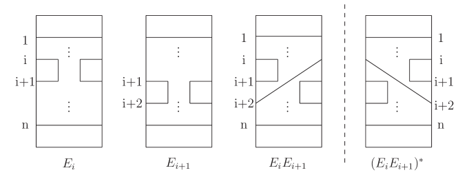
Figure 5: The generators $E_{i}$ and $E_{i+1}$ of the $TL_{n}$ algebra.

Here are the generators of the $TL_{n}(d)$ algebra:

$$E_{0}=(Id)^{\otimes(n)},\,\,E_{1}=P_{\ast}\otimes(Id)^{\otimes(n-2)},\,\,E_{2}=Id\otimes P_{\ast}\otimes(Id)^{\otimes(n-3)}$$

$$E_{i}=(Id)^{\otimes(i-1)}\otimes P_{\ast}\otimes(Id)^{\otimes(n-i-1)},\cdots,E_{n-1}=(Id)^{\otimes(n-2)}\otimes P_{\ast}.$$ (10)

See Figure 5 for their graphical representations.

2.2 Projectors and $D_{n}$ tangles

We construct projectors in terms of $Id$, $P$ and $P_{\ast}$. The operators $\frac{P_{\ast}}{d}$, $\frac{1\!\!1-P}{2}$ and $\frac{1}{2}(1\!\!1+P)-\frac{1}{d}P_{\ast}$ form a set of projection operators, satisfying

$$P_{1} = \frac{P_{\ast}}{d},\qquad P_{2}=\frac{1\!\!1-P}{2},\qquad P_{3}=\frac{1}{2}(1\!\!1+P)-\frac{1}{d}P_{\ast},$$

$$P_{1}^{2} = P_{1},\qquad P_{2}^{2}=P_{2},\qquad P_{3}^{2}=P_{3},$$

$$P_{1}P_{2} = 0,\qquad P_{1}P_{3}=0,\qquad P_{2}P_{3}=0,$$ (11)

$$P_{1}+P_{2}+P_{3}=1\!\!1.$$

The operators $\frac{P_{\ast}}{d}$ and $1\!\!1-\frac{P_{\ast}}{d}$ also form a set of projectors,

$$(\frac{P_{\ast}}{d})^{2}=\frac{P_{\ast}}{d},\qquad(1\!\!1-\frac{P_{\ast}}{d})^{2}=1\!\!1-\frac{P_{\ast}}{d},\qquad\frac{P_{\ast}}{d}(1\!\!1-\frac{P_{\ast}}{d})=0.$$ (12)

In addition, the operators $1\!\!1-\frac{2}{d}P_{\ast}$ and $P-\frac{2}{d}P_{\ast}$ are permutation-like,

$$(1\!\!1-\frac{2}{d}P_{\ast})^{2}=1\!\!1=P^{2}=(P-\frac{2}{d}P_{\ast})^{2}.$$ (13)

We extend our construction of projectors in terms of $Id$, $P$ and $P_{\ast}$ via the concept of the $D_{n}$ tangle. A $D_{n}$ tangle contains classical or virtual crossings with $n$ begin-points in a top row and $n$ end-points in a bottom row. Here the virtual crossing refers to permutation. A $D_{n}$ tangle without any crossings is also called an elementary tangle $T_{n}$ [29]. A $D_{n}$ tangle with only virtual crossings is called a virtual tangle $P_{n}$ [36]. We set up examples for the $T_{2}$ tangle, $P_{2}$ tangle and $D_{2}$ tangle in Figure 6.

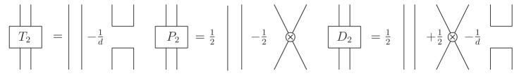
Figure 6: Projectors in terms of $2$ tangles.

Following a recursive procedure of deriving the Jones–Wenzl projector $T_{n}$ from a given $T_{2}$ diagram [29], we can generalize our construction $T_{2}$, $P_{2}$, $D_{2}$ to $T_{n}$, $P_{n}$, $D_{n}$, respectively.

At $d=2$, the operators $1\!\!1-P_{\ast}$ and $P-P_{\ast}$ are permutation-like. The operators $\frac{P_{\ast}}{2}$, $\frac{1\!\!1-P}{2}$ and $\frac{1\!\!1+P-P_{\ast}}{2}$ provide a set of projectors and operators $\frac{P_{\ast}}{2}$, $1\!\!1-\frac{P_{\ast}}{2}$ also. The projectors play basic roles in the Yang–Baxter theory, especially in six-vertex models [1]. A solution of the YBE in terms of the set of projectors simplifies involved calculation and make related geometric (algebraic) descriptions clear. We apply projectors via $P$ and $P^{\ast}$ to study new quantum algebras in eight-vertex models [16, 17]. Our results will appear elsewhere [37].

2.3 On the $TL_{n}$ algebra and $TL$ diagrams

One of the best known representations of the $TL$ algebra, where, in terms of diagrams, each cup and each cap is a Kronecker delta, has been used in lots of physics literature (e.g. Wu and collaborators on the intersecting string model for Potts type models [38, 39]). This representation gives a series of specializations of the Jones polynomial by making the variable in the bracket model fit the dimension of the representation (We also do some of this calculation in the present paper). Our work sets up a representation of the $TL$ algebra in terms of permutation’s partial transpose, which has a natural diagrammatic representation. It is worthwhile examining the potentiality of the partial transpose for setting up braid representations.

As a matter of fact, Figures 2–5 naturally exhibit $TL$ diagrams [29, 40]. They assign diagrammatical descriptions to the $TL_{n}$ algebra. Such a diagram is a planar $(n,n)$ diagram including a rectangle in the plane with $2n$ distinct points: $n$ on its left (top) edge and $n$ on its right (bottom) edge which are connected by disjoint strings drawn within in the rectangle. The identity is the diagram with all strings horizontal (vertical), while $E_{i}$ has its $i$th and $i+1$th left (top) (and right (bottom)) boundary points connected and all other strings horizontal (vertical). The multiplication $E_{i}E_{j}$ identifies right (bottom) points of $E_{i}$ with corresponding left (top) points of $E_{j}$, removes the common boundary and replaces each obtained loop with a factor $\chi$. The adjoint of $E^{\ast}_{i}$ is an image under mirror reflection of $E_{i}$ on a vertical (horizontal) line. So we have horizonal (vertical) $TL$ diagrams for showing the $TL$ algebra. Here, we take horizonal $TL$ diagrams for the multiplication of elements of the $TL$ algebra and vertical $TL$ diagrams for explaining braids or crossings.

3 The YBE solutions under dual symmetries

We sketch various formulations of the YBE and then study the Werner state [7], and the isotropic state [10] for examples of solutions of the YBE under dual symmetries. The Werner state has the form of $Id+uP$, $u$ being the parameter and its partial transpose is called the isotropic state $Id+uP_{\ast}$.

3.1 The YBEs and Yang–Baxterization

The YBE [8, 9] was originally found in the procedure of achieving exact solutions of two-dimensional quantum field theories or lattice models in statistical physics. It has the form

$$\check{R}_{i}(x)\,\check{R}_{i+1}(xy)\,\check{R}_{i}(y)=\check{R}_{i+1}(y)\,\check{R}_{i}(xy)\,\check{R}_{i+1}(x)$$ (14)

with the asymptotic condition $\check{R}_{i}(0)=\sigma_{i}$ and $x$ called the spectral parameter. In terms of new parameters $u,v$ given by $x=e^{u}$ and $y=e^{v}$, the YBE (14) has the other form

$$\check{R}_{i}(u)\,\check{R}_{i+1}(u+v)\,\check{R}_{i}(v)=\check{R}_{i+1}(v)\,\check{R}_{i}(u+v)\,\check{R}_{i+1}(u).$$ (15)

Furthermore, the algebraic YBE mentioned in the introduction reads

$$R_{12}(x)R_{13}(xy)R_{23}(y)=R_{23}(y)R_{13}(xy)R_{12}(x),$$ (16)

$R_{ij}$ acting on $V_{i}\otimes V_{j}$, which has a solution by $R(x)=\check{R}(x)P$.

Taking the limit of $x\to 0$ leads to the braid relation from the YBE (14) and the $\sigma$-matrix from the $\check{R}$-matrix. Note that both $\sigma_{i}$ and $\check{R}_{i}(x)$ are fixed up to an overall scalar factor. Concerning relations between the $\sigma$-matrix and $x$-dependent solutions of the YBE (14), we construct the $\check{R}(x)$-matrix from a given $\sigma$-matrix. Such a construction is called Yang–Baxterization [33]. It is important to make distinctions between the braid relations and YBEs. The braid relations are topological but the YBE relations are not necessarily topological due to the spectral parameter.

3.2 The Werner state and isotropic state

The Werner state $\rho_{W}$ [7] for a biparticle has the form

$$\rho_{W}=p\,|\psi^{-}\rangle\langle\psi^{-}|+\frac{1-p}{4}{1\!\!1}_{4}$$ (17)

where the symbol ${1\!\!1}_{4}$ is a four by four unit matrix and the Bell state $|\psi^{-}\rangle$ takes the form $|\psi^{-}\rangle=\frac{1}{\sqrt{2}}(|01\rangle-|10\rangle)$. So the Werner state $\rho_{W}$ has the form in matrix

$$\rho_{W}=\left(\begin{array}[]{cccc}\frac{1-p}{4}&0&0&0\\ 0&\frac{1+p}{4}&\frac{1-3p}{4}&0\\ 0&\frac{1-3p}{4}&\frac{1+p}{4}&0\\ 0&0&0&\frac{1-p}{4}\end{array}\right).$$ (18)

Set $p=\frac{1-2f}{3}$, then the Werner state $\rho_{W}$ is a linear combination of ${1\!\!1}_{4}$ and $P$, namely,

$$\rho_{W}=\frac{1}{6}((2-f){1\!\!1}_{4}+(2f-1)P)$$ (19)

which has a generalized form in $d$-dimension,

$$\rho_{W}=\frac{1}{d(d+1)}((d-f){1\!\!1}_{d}+(d\,f-1)P).$$ (20)

Choosing $u=\frac{df-1}{d-f}$, $f\neq d$, we obtain

$$\rho_{W}(u)=\frac{d-1}{d(u+d)}({1\!\!1}_{d}+u\,P)$$ (21)

which is a well known rational solution $\check{R}(u)$-matrix of the YBE (15). For a given $\check{R}(u)$-matrix, a standard “RTT” relation procedure [16, 17] specifies a Hamiltonian calculated by $H=\frac{d}{du}{\check{R}}(u)|_{u=0}$. The Werner state $\rho_{W}$ is related to a Hamiltonian given by

$$H=\sum_{i=1}^{N}P_{i,i+1}=\frac{1}{2}\sum_{i=1}^{N}(1\!\!1_{4}+\sigma^{x}_{i}\otimes\sigma^{x}_{i+1}+\sigma^{y}_{i}\otimes\sigma^{y}_{i+1}+\sigma^{z}_{i}\otimes\sigma^{z}_{i+1})$$ (22)

which is the Hamiltonian of the $XXX$ spin chain and where the Pauli matrices $\sigma^{x}$, $\sigma^{y}$ and $\sigma^{z}$ have the conventional formalism

$$\sigma^{x}=\left(\begin{array}[]{cc}0&1\\ 1&0\end{array}\right),\qquad\sigma^{y}=\left(\begin{array}[]{cc}0&-i\\ i&0\end{array}\right),\qquad\sigma^{z}=\left(\begin{array}[]{cc}1&0\\ 0&-1\end{array}\right).$$ (23)

The isotropic state $\rho_{I}$ is the partial transpose of the Werner state $\rho_{W}$,

$$\rho_{I}(v)=1\!\!1_{d}+vP_{\ast}=\Theta_{2}(\rho_{W}).$$ (24)

It forms a braid representation when the parameter $v$ satisfies

$$v_{\pm}=-\frac{1}{2}(d\mp\sqrt{d^{2}-4}),\qquad d\geq 2.$$ (25)

See the subsection 6.1 for the proof. The corresponding $\check{R}_{\pm}(u)$-matrix via Yang–Baxterization [41] has the form

$$\check{R}_{\pm}(u)=u\rho_{I}(v_{\pm})-u^{-1}\rho_{I}^{-1}(v_{\pm})=(uv_{\pm}-u^{-1}v_{\mp})+(u-u^{-1})P_{\ast},$$ (26)

which determines a local Hamiltonian with nearest neighbor interactions,

$$H_{i,i+1}=\frac{1}{2}1\!\!1_{4}+\frac{1}{2}(\sigma_{i}^{x}\otimes\sigma_{i+1}^{x}-\sigma_{i}^{y}\otimes\sigma_{i+1}^{y}+\sigma_{i}^{z}\otimes\sigma_{i+1}^{z}).$$ (27)

3.3 On the YBE solutions under dual symmetries

Classical invariant theory tells us that the linear combinations $aId+bP$ of identity and permutation are the only operators commuting with all unitary operators of the form $U\otimes U$. Similarly, the operators $aId+bP_{*}$ span the commutant of the operators $U\otimes\overline{U}$, where $\overline{U}$ denotes the complex conjugate of the matrix $U$ in the standard basis, which we have fixed throughout. Moreover, the linear combinations of $Id,P$ and $P_{*}$ span the commutant of the operators $U\otimes U$ with $U$ real orthogonal. These facts are heavily used in the characterization of symmetric states in quantum information theory, where the states with the two kinds of symmetry are called Werner states [7] and isotropic states [10], respectively [12].

It is very natural to look at such symmetries for constructing solutions of the braid and YBE relations. Indeed, we can require all $\check{R}(u)$ to commute with $U\otimes U$ for all unitaries in an appropriate subgroup $G$ of the unitary group. This property has then an immediate extension to relations on $n$ strands, and also automatically admits the ordinary permutation operators to serve as virtual generators. Obviously, the construction of solutions then proceeds by first decomposing the representation $U\otimes U$ into irreducible representations of $G$, typically leaving a much lower dimensional space in which to solve the required non-linear equations.

The choice of the operators $Id,P,P_{*}$ is by no means arbitrary, but reflects the choice of orthogonal symmetry as the underlying symmetry group $G$ for the single strand. Computations in the commutant of the operators $U^{\otimes n}$ on $n$ strands are simplified by choosing a basis, whose multiplication law can be represented graphically [13]. As usual, we can write a permutation $\pi$ as a (flat) braiding diagram, with $n$ strands going in at positions $(1,\ldots,n)$ and coming out at $(\pi_{1},\ldots,\pi_{n})$. This corresponds to the operator

$$V_{\pi}=\sum_{i_{1},\ldots,i_{n}}^{d}|i_{\pi_{1}}\cdots i_{\pi_{n}}\rangle\,\langle i_{1},\cdots,i_{n}|.$$ (28)

If we apply a partial transposition to any tensor factor, a pair of corresponding indices are swapped between the ket and the bra factor of each term. Thus we are still left with a sum over $n$ indices, each of which appears exactly twice, but the distribution of these $2n$ indices over ket and bra is completely arbitrary. The multiplication works exactly as for permutations, with the new feature that strands can turn back. Also closed loops can appear, which appear in the product only as a scalar factor $d$.

Note that such graphical representations are the Brauer diagrams since the Brauer algebra $D_{n}$ [11] maps surjectively to the commutant of the action of the orthogonal group on the tensor powers of its representation. The Brauer diagrams are similar to the $TL$ diagrams but allow strings to intersect. The next section focuses on the Brauer algebra and the $PPT_{n}$ algebra generated by permutation’s partial transposes.

4 The $PPT_{n}$ algebra and Brauer algebra

In terms of $Id$, $P$ and $P_{\ast}$, we can set up multipartite symmetric states under transformations of unitary group, orthogonal group and the tensor product of unitary group and its complex conjugation. Since the Peres–Horodecki criterion [4, 5] involves a state and its partial transpose, we figure out the set of permutation’s partial transposes and articulate it as the $PPT$ algebra. This algebra plus permutations whose partial transposes are not themselves is isomorphic to the Brauer algebra [11]. Here we define the $PPT_{n}$ algebra, explain it with examples, sketch the axioms of the Brauer algebra and draw Brauer diagrams to show permutation and its partial transpose.

4.1 The $PPT_{n}$ algebra

The transpose $\Theta$ in the $n$-fold finite dimensional Hilbert space ${\cal H}^{\otimes n}$ is defined by its action on a given operator

$$\Theta(|i_{1}i_{2}\cdots i_{n}\rangle\langle j_{1}j_{2}\cdots j_{n}|)=|j_{1}j_{2}\cdots j_{n}\rangle\langle i_{1}i_{2}\cdots i_{n}|,$$ (29)

while the partial transpose $\Theta_{k}$, $1\leq k\leq n$ takes the action,

$$\Theta_{k}(|i_{1}\cdots i_{k}\cdots i_{n}\rangle\langle j_{1}\cdots j_{k}\cdots j_{n}|)=|j_{1}\cdots j_{k}\cdots j_{n}\rangle\langle i_{1}\cdots i_{k}\cdots i_{n}|,$$ (30)

so that the multi-partial transpose $\Theta_{l_{1}l_{2}\cdots\,l_{j}}$ is defined as

$$\Theta_{l_{1}l_{2}\cdots\,l_{j}}=\Theta_{l_{1}}\Theta_{l_{2}}\cdots\Theta_{l_{j}},\qquad\Theta=\prod_{i=1}^{n}\Theta_{k},\qquad 1\leq j<n.$$ (31)

Note that the set of $\Theta_{k}$ forms an abelian group defined by $\Theta_{k}^{2}=Id,\Theta_{i}\Theta_{j}=\Theta_{j}\Theta_{i}$.

The symmetric group $S_{n}$ consists of all possible permutations of $n$-objects. Its group algebra ${\cal S}_{n}$ is generated by cyclic permutations $\pi_{i}=(i,i+1)$ and $Id$, satisfying

$$\pi_{i}\pi_{i+1}\pi_{i} = \pi_{i+1}\pi_{i}\pi_{i+1},\qquad i=1,\cdots,n-1,$$

$$\pi_{i}^{2} = Id,\qquad\pi_{i}\pi_{j}=\pi_{j}\pi_{i},\qquad j\neq i\pm 1.$$ (32)

Denote an operator $V_{j}$ in ${\cal H}^{\otimes n}$ in terms of Dirac’s bras and kets,

$$V_{j}=\sum_{i_{1},\ldots,i_{n}}^{d}|i_{1},\cdots,i_{j+1}i_{j},\cdots i_{n}\rangle\,\langle i_{1},\cdots,i_{j}i_{j+1},\cdots,i_{n}|$$ (33)

which satisfies the following relations given by

$$V_{i}V_{i+1}V_{i} = V_{i+1}V_{i}V_{i+1},\qquad i=1,\cdots,n-1,$$

$$V_{i}^{2} = Id,\qquad V_{i}V_{j}=V_{j}V_{i},\qquad j\neq i\pm 1$$ (34)

so that the set of $V_{j}$ forms a representation of the symmetry group algebra ${\cal S}_{n}$.

The action of $\Theta_{j}$ on $V_{j}$ leads to an idempotent $E_{j}$ given by

$$E_{j}=\Theta_{j}(V_{j})=\sum_{i_{1},\ldots,i_{n}}^{d}|i_{1},\cdots,i_{j}i_{j},\cdots i_{n}\rangle\,\langle i_{1},\cdots,i_{j+1}i_{j+1},\cdots,i_{n}|$$ (35)

satisfying the $TLR(d)$ relation with the loop parameter $d$ similar to the permutation’s partial transpose $P_{\ast}$ presented before. The $PPT_{n}(i)$ algebra denoting the action of $\Theta_{i}$ on the ${\cal S}_{n}$ algebra have the generators as

$$V_{1},V_{2},\cdots,E_{i-1},E_{i},\cdots V_{n-1}.$$ (36)

For the multi-partial transpose $\Theta_{l_{1}l_{2}\cdots\,l_{j}}$, the $PPT_{n}(l_{1}l_{2}\cdots l_{j})$ algebra is generated in the same way as the $PPT_{n}(i)$ algebra. The $PPT_{n}(i)$ algebra is isomorphic to the symmetric group algebra ${\cal S}_{n}$ generated by $Id$ and $V_{j}$ since their generators are in one to one correspondence by $V_{i-1}\to E_{i-1}$, $V_{i}\to E_{i}$. The $\Theta_{k}$ acting on the product $V_{i}V_{j}$ has the form

$$\Theta_{k}(V_{i}^{2}) = Id,\qquad\Theta_{k+1}(V_{k}V_{k+1})=\Theta_{k+1}(V_{k+1})\Theta_{k+1}(V_{k})$$

$$\Theta_{k}(V_{i}V_{j}) = \Theta_{k}(V_{i})\Theta_{k}(V_{j}),\qquad\textrm{for other cases}$$ (37)

which show that $\Theta_{1}$ is a homomorphism between the generators of ${\cal S}_{n}$ and those of $PPT_{n}$, the transpose $\Theta$ is an anti-homomorphism but the $\Theta_{k},k\geq 2$ is neither homomorphism nor anti-homomorphism.

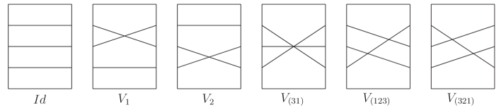
Figure 7: Brauer diagrams for the symmetric group algebra ${\cal S}_{3}$.

The Brauer algebra is generated by $TL$ idempotents and virtual crossings (i.e., permutations) and it can be also generated by a $TL$ idempotent plus the symmetric group algebra ${\cal S}_{n}$. For example, the idempotent $E_{i}$ is related to $E_{i-1}$ in the way

$$\Theta_{i}(V_{i})=E_{i}=V_{i-1}V_{i}E_{i-1}V_{i}V_{i-1}=V_{i-1}V_{i}\Theta_{i}(V_{i-1})V_{i}V_{i-1}.$$ (38)

So the $PPT_{n}(i)$ algebra at $n>2$ is a subalgebra of the Brauer algebra. The $PPT_{n}(i)$ algebra together with $V_{i-1}$ and $V_{i}$ denoted by the $\overline{PPT}_{n}(i)$ algebra is isomorphic to the Brauer algebra, similarly for the algebra $\overline{PPT}_{n}(l_{1}l_{2}\cdots l_{j})$.

4.2 Examples for the $PPT_{n}$ algebra

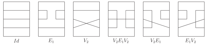
Figure 8: Brauer diagrams for the $PPT_{3}$ algebra.

The symmetric group $S_{3}$ is the set given by

$$S_{3}=\{e,(12),(23),(31),(123),(321)\}$$ (39)

including the identity $e$. It has two generators $\pi_{1}$ and $\pi_{2}$ yielding the other elements by

$$(13)=\pi_{2}\pi_{1}\pi_{2},\,\,(123)=\pi_{2}\pi_{1},\,\,(321)=\pi_{1}\pi_{2}.$$ (40)

Introduce a representation of ${\cal S}_{3}$ via a map

$$D:\pi\to V_{\pi}=\sum_{i,j,k=1}^{d}|\pi(ijk)\rangle\langle ijk|,\qquad\pi\in S_{3}$$ (41)

and every $V_{\pi}$ has its own Brauer diagram, see Figure 7.

Figure 9: The transformation between two idempotents $E_{1}$ and $E_{2}$.

The partial transpose $\Theta_{1}$ is a homomorphism between ${\cal S}_{3}$ and $PPT_{3}(1)$, see Figure 8,

$$E_{1} = \Theta_{1}(V_{(12)}),\qquad V_{2}=\Theta_{1}(V_{(23)})=V_{(23)},\qquad\Theta_{1}(V_{(13)})=V_{2}E_{1}V_{2},$$

$$Id = \Theta(V_{e}),\qquad\Theta_{1}(V_{(123)})=V_{2}E_{1},\qquad\Theta_{1}(V_{(321)})=E_{1}V_{2}$$ (42)

where the generator $E_{1}$ is an idempotent and the other generator $V_{2}$ is a permutation,

$$E_{1}^{2}=dE_{1},\qquad V_{2}^{2}=1\!\!1,\qquad E_{1}V_{2}E_{1}=V_{2}.$$ (43)

The $PPT_{3}(1)$ algebra, generated by $Id$, $E_{1}$ and $V_{2}$, and $V_{1}$ form the $\overline{PPT}_{3}(1)$ algebra which is isomorphic to the Brauer algebra $D_{3}(d)$. For example, the idempotent $E_{2}$ of $D_{3}(d)$ can be generated by $V_{(13)}E_{1}V_{(13)}$ and $V_{(13)}=V_{1}V_{2}V_{1}$, see Figure 9. The $PPT_{3}(1)$ algebra minus the generator $V_{2}$ is isomorphic to the $TL_{2}(d)$ algebra.

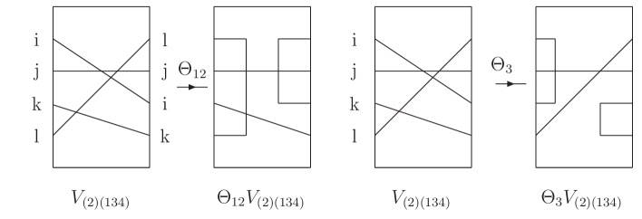
Figure 10: Brauer diagrams for partial transposes in the $PPT_{4}$ algebra.

At $n=4$, consider the permutation element $(2)(134)$ of the symmetric group $S_{4}$. The partial transpose $\Theta_{12}$ denotes the transpose in the first and second Hilbert spaces. They have the following presentations

$$V_{(2)(134)}=\sum_{i,j,k,l=1}^{d}|ljik\rangle\langle ijkl|,\qquad\Theta_{12}V_{(2)(134)}=\sum_{i,j,k,l=1}^{d}|ijik\rangle\langle ljkl|.$$ (44)

See Figure 10. In terms of Brauer diagrams, we calculate the product $V_{(2)(134)}\Theta_{12}V_{(2)(134)}$ and recognize it as the adjoint of $\Theta_{3}V_{(2)(134)}$ where $\Theta_{3}$ denotes the transpose in the third Hilbert space,

$$\Theta_{3}V_{(2)(134)}=\sum_{i,j,k,l=1}^{d}|ljkk\rangle\langle ijil|,$$ (45)

and we also show $\Theta_{12}V_{(2)(134)}$ to be an idempotent which allows intersecting strings, see Figure 11.

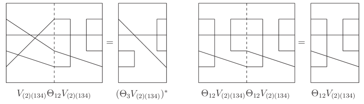
Figure 11: Brauer diagrams for multiplications in the $PPT_{4}$ algebra

4.3 The axioms of the Brauer algebra

Here we list the axioms of the Brauer algebra $D_{n}(x)$ [11]. The parameter $x$ called the loop parameter takes the dimension $d$ in this paper. Its generators have $TL$ idempotents $E_{i}$ and virtual crossings $v_{i}$, $i=1,\cdots,n-1$, see Figure 12.

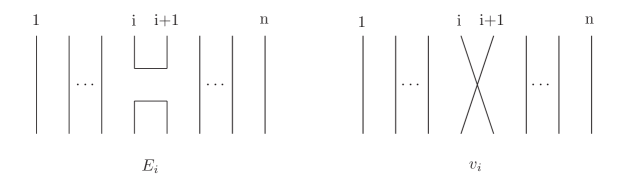
Figure 12: Generators $E_{i}$ and $v_{i}$ of the Brauer algebra.

$TL$ idempotents $E_{i}$ satisfy the $TLR(x)$ relation (2.1) and virtual crossings $v_{i}$ are defined by the virtual crossing relation denoted by “$VCR$”,

$$VCR:\,\,v_{i}^{2} = 1\!\!1,\qquad v_{i}v_{i+1}v_{i}=v_{i+1}v_{i}v_{i+1},$$

$$v_{i}v_{j} = v_{j}v_{i},\qquad j\neq i\pm 1.$$ (46)

They satisfy the mixed relations by

$$(ev/ve):E_{i}v_{i}=v_{i}E_{i}=E_{i},\qquad E_{i}v_{j}=v_{j}E_{i},\qquad j\neq i\pm 1,$$

$$(vee):v_{i\pm 1}E_{i}E_{i\pm 1}=v_{i}E_{i\pm 1},\qquad(eev):E_{i\pm 1}E_{i}v_{i\pm 1}=E_{i\pm 1}v_{i},$$ (47)

for example, see Figure 13 for the $(eev)$ axiom. The Brauer algebra generated by idempotents $E_{i}$ and virtual crossings $v_{i}$ are defined by the $TLR(x)$, $VCR$, $(ev/ve)$, $(vee)$ and $(eev)$ relations. These defining axioms can drive the other mixed relations. The axioms $(vee)$ and $(eev)$ lead to the $(vee)$ and $(evv)$ relations, respectively,

$$(vee)\Rightarrow(vve):v_{i\pm 1}v_{i}E_{i\pm 1}=E_{i}E_{i\pm 1},$$

$$(eev)\Rightarrow E_{i}E_{i\pm 1}E_{i}v_{i\pm 1}=E_{i}E_{i\pm 1}v_{i}\Rightarrow(evv):E_{i}v_{i\pm 1}v_{i}=E_{i}E_{i\pm 1}.$$ (48)

Identifying $(vve)$ with $(evv)$ leads to the $(vev)$ relation,

$$(vve),(evv)\Rightarrow v_{i\pm 1}v_{i}E_{i\pm 1}=E_{i}v_{i\pm 1}v_{i}\Rightarrow(vev):v_{i\pm 1}E_{i}v_{i\pm 1}=v_{i}E_{i\pm 1}v_{i}.$$ (49)

Furthermore, the relations $(vev)$ and $(vve)$ suggest the relation $(eve)$,

$$(vev)\Rightarrow E_{i}v_{i\pm 1}E_{i}=v_{i\pm 1}v_{i}E_{i\pm 1}E_{i}=E_{i}E_{i\pm 1}E_{i}\Rightarrow(eve):E_{i}v_{i\pm 1}E_{i}=E_{i}.$$ (50)

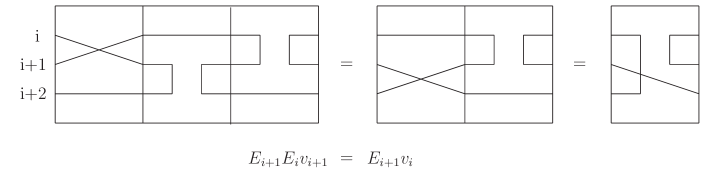
Figure 13: The $(eev)$ axiom of the Brauer algebra.

At the diagrammatical level, it is explicit that the permutation $P$ and its partial transpose $P_{\ast}$ form the Brauer algebra. Introduce a new permutation notation $P^{\pm}$ and denote $Q_{\ast}$ as a $q$ deformation of permutation’s partial transpose $P_{\ast}$. They have the forms

$$P^{\pm}=\left(\begin{array}[]{cccc}1&0&0&0\\ 0&0&\pm 1&0\\ 0&\pm 1&0&0\\ 0&0&0&1\end{array}\right),\qquad Q_{\ast}=\left(\begin{array}[]{cccc}1&0&0&-q\\ 0&0&0&0\\ 0&0&0&0\\ -q^{-1}&0&0&1\end{array}\right).$$ (51)

We check that $P^{\pm}$ and $Q_{\ast}$ form the Brauer algebra. The $Q_{\ast}$ is a $TL$-idempotent satisfying

$$Q_{\ast}Q_{\ast}=2Q_{\ast},\qquad Q_{\ast i}Q_{\ast i\pm 1}Q_{\ast i}=Q_{\ast i}$$ (52)

and the hermitian $Q_{\ast}$ requires the deformed parameter $q$ living at the unit circle. The three mixed relations for the defining axioms are verified by

$$P^{\pm}Q_{\ast} = Q_{\ast}P^{\pm}=Q_{\ast},$$

$$P_{i}^{\pm}Q_{\ast i+1}Q_{\ast i} = P^{\pm}_{i+1}Q_{\ast i},\qquad Q_{\ast i+1}Q_{\ast i}P^{\pm}_{i+1}=Q_{\ast i+1}P^{\pm}_{i}.$$ (53)

Note that in the following sections we will focus on $P_{\ast}$ instead of $Q_{\ast}$ since they behave in the same way. The Brauer algebra is a limit of the Birman–Wenzl algebra [42, 43] in which the defining axioms and derived mixed relations are independent of each other. The Birman–Wenzl algebra was devised to explain the Kauffman two variable polynomial in terms of its trace functional.

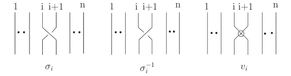
Figure 14: The braid generators and virtual braid generator.

5 The virtual, welded and unrestricted braid groups

Besides the commutant of the tensor power of the orthogonal group, $PPT_{n}$ algebra and Brauer algebra, there are the virtual knot theory and its underlying virtual $TL$ algebra via permutation and its partial transpose. We sketch the axioms defining the family of virtual braids, then construct the virtual braid representations in terms of the linear combination of $Id$, $P$ and $P_{\ast}$.

The classical braid group $B_{n}$ (the Artin braid group) on $n$ strands is generated by the braids $\sigma_{i}$ and it consists of all words of the form $\sigma_{j_{1}}^{\pm 1}\sigma_{j_{2}}^{\pm 1}...\sigma_{j_{n}}^{\pm 1}$ modulo the braid relations, see Figures 14-15:

$$BGR:\,\,\sigma_{i}\sigma_{i+1}\sigma_{i} = \sigma_{i+1}\sigma_{i}\sigma_{i+1},\qquad i=1,\cdots,n-1,$$

$$\sigma_{i}\sigma_{j} = \sigma_{j}\sigma_{i},\qquad j\neq i\pm 1,$$ (54)

which is denoted as “$BGR$” for the braid group relation.

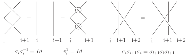
Figure 15: Identity and the braid relation.

The virtual braid group $VB_{n}$ [24, 25, 26, 27] is an extension of the classical braid group $B_{n}$ by the symmetric group $S_{n}$. It has both the braids $\sigma_{i}$ and virtual crossings $v_{i}$. A virtual crossing $v_{i}$ is represented by two crossing arcs with a small circle placed around the crossing point. In virtual crossings, we do not distinguish between under and over crossing but which are described respectively in the classical knot theory.

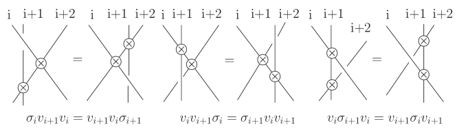
Figure 16: The virtual braid relations.

The virtual generators $v_{i}$ satisfy the $VCR$ relation (4.3) and they form a representation of the symmetric group $S_{n}$. The virtual generators $v_{i}$ and braid generators $\sigma_{j}$ satisfy the mixed relations:

$$VBR:\,\,\sigma_{i}v_{j} = v_{j}\sigma_{i},\qquad j\neq i\pm 1,$$

$$v_{i}\sigma_{i+1}v_{i} = v_{i+1}\sigma_{i}v_{i+1},$$ (55)

which is denoted as “$VBR$” for the virtual braid relation. Here the second mixed relation is also called the special detour relation.

There are the following relations also called special detour moves for virtual braids and they are easy consequences of (4.3) and (5), see Figure 16:

$$\sigma_{i}^{\pm}v_{i+1}v_{i} = v_{i+1}v_{i}\sigma_{i+1}^{\pm},$$

$$v_{i}v_{i+1}\sigma_{i}^{\pm} = \sigma_{i+1}^{\pm}v_{i}v_{i+1},$$

$$v_{i}\sigma_{i+1}^{\pm}v_{i} = v_{i+1}\sigma_{i}^{\pm}v_{i+1}.$$ (56)

This set of relations taken together defines the basic isotopies for virtual braids.

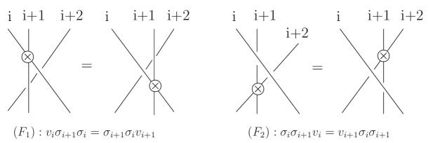
Figure 17: The forbidden moves: $(F_{1})$ and $(F_{2})$.

The move with two real crossings and one virtual crossing is a forbidden move in the virtual knot theory. However, there are two types of forbidden moves: the one with an over arc denoted by $(F_{1})$ and the other with an under arc denoted by $(F_{2})$,

$$(F_{1}):v_{i}\sigma_{i+1}\sigma_{i}=\sigma_{i+1}\sigma_{i}v_{i+1},\qquad(F_{2}):\sigma_{i}\sigma_{i+1}v_{i}=v_{i+1}\sigma_{i}\sigma_{i+1},$$ (57)

see Figure 17. The first forbidden move $(F_{1})$ preserves the combinatorial fundamental group, as is not true for the second forbidden move $(F_{2})$. This makes it possible to take an important quotient of the virtual braid group $VB_{n}$. The welded braid group $WB_{n}$ on $n$ strands [44] satisfies the same isotopy relations as the $VB_{n}$ group but allows the forbidden move $(F_{1})$. The unrestricted virtual braid group $UB_{n}$ allows the forbidden moves $(F_{1})$ and $(F_{2})$ although any classical knot can be unknotted in the virtual category if we allow both forbidden moves [45, 46]. Nevertheless, linking phenomena still remain.

The shadow of some link in three dimensional space without specifying the weaving of that link is a link or knot diagram which does not distinguish the over crossing from the under one. The shadow crossing without regard to the types of crossing is called a flat crossing. The flat virtual braid group $FV_{n}$ [25] consists of virtual crossings $v_{i}$ and flat crossings $c_{i}$. It satisfies the same relations as the $VB_{n}$ except the braid $\sigma_{i}$ replaced with the flat crossing $c_{i}$ satisfying $c_{i}^{2}=1\!\!1$. The generalization of the $FV_{n}$ is called the flat unrestricted braid group $FU_{n}$. It is the quotient of the $FV_{n}$ by adding the forbidden move of $FV_{n}$. Note that for the $FV_{n}$ there is only one type of forbidden move since here $(F_{1})$ is the same as $(F_{2})$, see,

$$(F_{1})\Rightarrow\sigma_{i+1}v_{i}\sigma_{i+1}=\sigma_{i}v_{i+1}\sigma_{i}\Rightarrow(F_{2}).$$ (58)

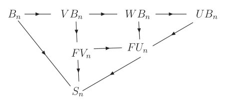
Figure 18: Relationships among various braid groups.

The flat unrestricted braid group $FU_{n}$ is a quotient of the welded braid group $WB_{n}$, obtained by setting all the squares of the braiding generators equal to $1\!\!1$. Thus there is a surjective homomorphism from $WB_{n}$ to $FU_{n}.$ This homomorphism is a direct analogue of the standard homomorphism from the braid group $B_{n}$ to the symmetric group $S_{n}$. Figure 18 draws a commutative diagram of these relationships where all structures map eventually to the symmetric group $S_{n}$ [47].

6 The virtual braid representations via $P$ and $P_{\ast}$

We set up virtual braid representations in terms of $Id$, $P$ and $P_{\ast}$. The isotropic state $Id+v_{\pm}P_{\ast}$ satisfies the braid relation. The braid (virtual crossing) $1\!\!1-P_{\ast}$ and virtual crossing (braid) $P$ form flat unrestricted braid representations which underlie common solutions of the braid relation and YBEs. The linear combination of $1\!\!1-P_{\ast}$ and $P$ leads to a family of unitary braid representations with adjustable parameters.

6.1 The braid representation via permutation’s partial transpose

Denote the operator $1\!\!1+vP_{\ast},v\neq 0$ by $\check{R}(v)$. Substituting $\check{R}(v)$ into both sides of the braid relation (5), we obtain

$$\check{R}_{i}(v)\check{R}_{i+1}(v)\,\check{R}_{i}(v)|ijk\rangle=|ijk\rangle+(2v+v^{3}+dv^{2})\sum_{l=1}^{d}|llk\rangle\delta_{ij}$$

$$+v\sum_{l=1}^{d}|ill\rangle\delta_{jk}+v^{2}\sum^{d}_{l=1}|kll\rangle\delta_{ij}+v^{2}\sum_{l=1}^{d}|lli\rangle\delta_{jk},$$

$$\check{R}_{i+1}(v)\,\check{R}_{i}(v)\,\check{R}_{i+1}(v)|ijk\rangle=|ijk\rangle+(2v+dv^{2}+v^{3})\sum_{l=1}^{d}|ill\rangle\delta_{jk}$$

$$+v\sum_{l=1}^{d}|llk\rangle\delta_{ij}+v^{2}\sum_{l=1}^{d}|lli\rangle\delta_{jk}+v^{2}\sum_{l=1}^{d}|kll\rangle\delta_{ij}.$$ (59)

Identifying both sides leads to an equation of the variable $v$,

$$2v+dv^{2}+v^{3}=v\Rightarrow v+v^{-1}=-d$$ (60)

which has solutions $v_{\pm}$ given by (25). So $1\!\!1+v_{\pm}P_{\ast}$ or $v_{\mp}\,1\!\!1+P_{\ast}$ forms a family of braid representations. The $P_{\ast}$ itself does not form a braid representation since the terms with the coefficient $v^{3}$ on both sides are different. In addition, the operator $\check{R}(v)$ is not a solution of the YBE (14) or (15). But $1\!\!1+uP,u\neq 0$ is a rational solution of the YBE (14) but not a solution of the braid relation. Note the calculation

$$(\check{R}(v))^{2}=1\!\!1+v(2+vd)P_{\ast}=\check{R}(v)+v(1+vd)P_{\ast}.$$ (61)

It says: at $v=-\frac{1}{d}$, the $\check{R}(v)$ is a projector; at $v=-\frac{2}{d}$, the $\check{R}(v)$ is permutation-like, and represents a braid only for $d=2$.

Note that a solution of the braid relation can be constructed in terms of a $TL$ idempotent, see the appendix A for the detail. Here we have $\check{R}_{\pm}=v_{\mp}1\!\!1+P_{\ast}$ so that the Hecke condition [41] is satisfied by

$$(\check{R}_{\pm})^{2}=(v_{\pm}-v_{\mp}){\check{R}_{\pm}}+1\!\!1,\qquad v_{\pm}+({v_{\pm}})^{-1}=-d.$$ (62)

Note that for $d=3$ the orthogonal group coincides with the spin-$1$ representation of $SU(2)$. The basic technique of using strand symmetry can of course also be extended to higher spin representations of $SU(2)$. For example, at spin $3/2$, we get a four dimensional commutant, in which the braid relation can be solved.

6.2 Flat unrestricted braid representations

In [24], remarks about quantum link invariants show that any braid group representation defined in the usual way by a solution to the braid version of the YBE (ie. a solution to the YBE that satisfies the braid relation) extends to a representation of the virtual braid group when the virtual generator is represented by the permutation (swap gate). Therefore the braid $1\!\!1+v_{\pm}P_{\ast}$ and the virtual crossing $P$ form a representation of the $VB_{2}$ group.

We construct a flat unrestricted braid representation $FU_{2}$. At $d=2$ and $u=-1$, the operator $1\!\!1-P_{\ast}$ denoted by $P^{\ast}$ forms a braid representation,

$$P^{\ast}=1\!\!1-\,P_{\ast}=\left(\begin{array}[]{cccc}0&0&0&-1\\ 0&1&0&0\\ 0&0&1&0\\ -1&0&0&0\end{array}\right),\qquad P^{\ast}P^{\ast}=1\!\!1.$$ (63)

and $P$ The $P_{\ast}$ acting on a state $|\xi\eta\rangle$ lead to

$$P|\xi\eta\rangle=|\eta\xi\rangle,\qquad P_{\ast}|\xi\eta\rangle=\sum_{l=0}^{1}|ll\rangle\delta_{\xi\eta},\qquad\xi,\eta=0,1,$$ (64)

so that the action of $P^{\ast}$ on $|ij\rangle$ takes the form

$$P^{\ast}|ij\rangle=|ij\rangle-(|00\rangle+|11\rangle)\delta_{ij}.$$ (65)

In terms of $P$ and $P^{\ast}$, we verify the following equalities:

$$P_{i}P_{i+1}P_{i}=P_{i+1}P_{i}P_{i+1},\qquad P^{\ast}_{i}P^{\ast}_{i+1}P^{\ast}_{i}=P^{\ast}_{i+1}P^{\ast}_{i}P^{\ast}_{i+1},$$ (66)

which proves that $P$ and $P^{\ast}$ form braid representations;

$$P_{i}^{2} = (P^{\ast}_{i})^{2}=1\!\!1,\qquad P_{i}P^{\ast}_{i+1}P_{i}=P_{i+1}P^{\ast}_{i}P_{i+1},$$

$$P_{i}P^{\ast}_{i+1}P^{\ast}_{i} = P^{\ast}_{i+1}P^{\ast}_{i}P_{i+1},\qquad P^{\ast}_{i}P^{\ast}_{i+1}P_{i}=P_{i+1}P^{\ast}_{i}P^{\ast}_{i+1},$$ (67)

which proves that the flat crossing $P^{\ast}$ and virtual crossing $P$ form a flat unrestricted braid representation $FU_{2}$;

$${P^{\ast}_{i}}^{2} = P_{i}^{2}=1\!\!1,\qquad P^{\ast}_{i}P_{i+1}P^{\ast}_{i}=P^{\ast}_{i+1}P_{i}P^{\ast}_{i+1},$$

$$P^{\ast}_{i}P_{i+1}P_{i} = P_{i+1}P_{i}P^{\ast}_{i+1},\qquad P_{i}P_{i+1}P^{\ast}_{i}=P^{\ast}_{i+1}P_{i}P_{i+1},$$ (68)

which proves the flat crossing $P$ and virtual crossing $P^{\ast}$ form the other flat unrestricted braid representation $FU_{2}$. Note that in higher dimensional ($d>2$) cases, substitute the braid $1\!\!1+v_{\pm}P_{\ast}$ and virtual crossing $P$ into two forbidden moves (57), we find that they are not satisfied at $d>2$. Also, the $1\!\!1+v_{\pm}P_{\ast}$ can not set up a flat braid representation for $d>2$.

6.3 Common solutions of (14), (15) and (5)

We consider the linear combination of $Id$, $P$ and $P_{\ast}$ by

$$\check{R}(u)=a1\!\!1+uP+bP_{\ast}.$$ (69)

Theorem 1 (below) presents a family of common solutions of the braid relation (5) and YBEs (14) and (15). See Figure 19.

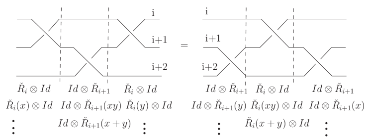
Figure 19: A common solution of the braid relation and YBEs.

Theorem 1. The $\check{R}(u)$ operator (69) forms a braid representation (5) only for $d=2,a=-b$ or $a=b=-u$ at $a\neq 0$ and it satisfies the YBE (14) or (15) only for $d=2,a=-b$ at $a\neq 0$, the coefficient of $P$ as the spectral parameter.

Before proving Theorem 1, we make the statements of Theorem 1 clear. The coefficient of $P_{\ast}$ being the spectral parameter leads to trivial results. For $a=b=-u$ and $d=2$, the $\check{R}(u)$-matrix has the form

$$\check{R}=1\!\!1-P+P_{\ast}=\left(\begin{array}[]{cccc}1&0&0&1\\ 0&1&-1&0\\ 0&-1&1&0\\ 1&0&0&1\\ \end{array}\right)$$ (70)

which is a known symmetric solution of the eight-vertex model. For $d=2,a=-b$, the $\check{R}(u)$-matrix takes the form

$$\check{R}(u)=aP^{\ast}+uP=\left(\begin{array}[]{cccc}u&0&0&-a\\ 0&a&u&0\\ 0&u&a&0\\ -a&0&0&u\end{array}\right),$$ (71)

which is a symmetric eight-vertex model with a parameter $u$ and also satisfies the YBEs (14) and (15), $u$ as the spectral parameter.

Note that the braid $\check{R}(u)$-matrix (71) and the virtual crossing $P$ form a unrestricted braid representation of $UB_{2}$. They satisfy both forbidden moves (57) but the $\check{R}(u)$-matrix has its square by

$$\check{R}(u)^{2}=(a^{2}+u^{2})+2au(P+P^{\ast}).$$ (72)

which is proportional to $Id$ only at $au=0$.

Now we present the proof for Theorem 1.

Proof. The proof has two parts. The first indicates that in higher ($d>2$) dimension the $\check{R}(u)$ operator (69) leads to trivial conclusions. We have to calculate all matrix entries of both sides of (5), (14) and (15) and then compare them one by one, see the appendix B for details.

The second verifies that at $d=2$ the $\check{R}(u)$-matrix (71) forms common solutions of (5), (14) and (15). The proof uncovers that flat unrestricted braid representations generated by (66), (6.2), (6.2) underlie the existence of common solutions of the braid relation (5) and YBEs (14), (15). After a little algebra, we have

$$\check{R}_{i}(x)\check{R}_{i+1}(z)\check{R}_{i}(y)=a^{3}P_{i}^{\ast}P^{\ast}_{i+1}P^{\ast}_{i}+xyzP_{i}P_{i+1}P_{i}$$ (73)

$$+ a^{2}yP^{\ast}_{i}P^{\ast}_{i+1}P_{i}+a^{2}zP_{i}^{\ast}P_{i+1}P_{i}^{\ast}+a^{2}xP_{i}P^{\ast}_{i+1}P^{\ast}_{i}$$

$$+ ayzP^{\ast}_{i}P_{i+1}P_{i}+axyP_{i}P_{i+1}^{\ast}P_{i}+axzP_{i}P_{i+1}P^{\ast}_{i},$$

$$\check{R}_{i+1}(y)\check{R}_{i}(z)\check{R}_{i+1}(x)=a^{3}P^{\ast}_{i+1}P^{\ast}_{i}P^{\ast}_{i+1}+xyzP_{i+1}P_{i}P_{i+1}$$

$$+ a^{2}xP^{\ast}_{i+1}P^{\ast}_{i}P_{i+1}+a^{2}zP^{\ast}_{i+1}P_{i}P^{\ast}_{i+1}+a^{2}yP_{i+1}P^{\ast}_{i}P^{\ast}_{i+1}$$

$$+ axzP^{\ast}_{i+1}P_{i}P_{i+1}+axyP_{i+1}P^{\ast}_{i}P_{i+1}+ayzP_{i+1}P_{i}P^{\ast}_{i+1}$$

which shows that the $\check{R}(u)$-matrix satisfies the following equation

$$\check{R}_{i}(x)\check{R}_{i+1}(z)\check{R}_{i}(y)=\check{R}_{i+1}(y)\check{R}_{i}(z)\check{R}_{i+1}(x).$$ (74)

We finish the proof by replacing the symbol $z$ with $xy$ or $x+y$ and requiring $x=y=z$. In addition, the equation (74) is related to the coloured Yang–Baxter equation [34].

$\hfill\Box$

6.4 Unitary braid representations via Yang–Baxterization

There is a bigger family of common solutions satisfying (5), (14) and (15). We derive it via Yang–Baxterization [33]. The $\check{R}(u)$-matrix (71) divided by a scaling factor $a$ has the form, which is an example of a general $\check{R}_{\pm}$-matrix by

$$\check{R}=\left(\begin{array}[]{cccc}t&0&0&-1\\ 0&1&t&0\\ 0&t&1&0\\ -1&0&0&t\\ \end{array}\right),\qquad t=\frac{u}{a},\qquad\check{R}_{\pm}=\left(\begin{array}[]{cccc}t&0&0&q\\ 0&1&\pm t&0\\ 0&\pm t&1&0\\ q^{-1}&0&0&t\\ \end{array}\right),$$ (75)

$q$ being the deformation parameter. The $\check{R}_{\pm}$-matrix has three distinguished eigenvalues:

$$\lambda_{1}=1+t,\,\,\,\lambda_{2}=1-t,\,\,\,\lambda_{3}=t-1.$$ (76)

Via Yang–Baxterization, the corresponding $\check{R}_{\pm}(x)$-matrix is obtained to be

$$\check{R}_{\pm}(x) = \check{R}_{\pm}+x(1-t^{2})\check{R}_{\pm}^{-1}$$ (81)

$$= \left(\begin{array}[]{cccc}t(1-x)&0&0&q(1+x)\\ 0&1+x&\pm t(1-x)&0\\ 0&\pm t(1-x)&1+x&0\\ q^{-1}(1+x)&0&0&t(1-x)\\ \end{array}\right).$$

The unitarity condition, with the normalization factor denoted by $\rho$,

$$\check{R}_{\pm}(x)\check{R}_{\pm}^{\dagger}(\bar{x})=\check{R}_{\pm}^{\dagger}(\bar{x})\check{R}_{\pm}(x)=\rho 1\!\!1,$$ (82)

leads to $\|q\|^{2}=1$ and $\|x\|^{2}=1$ for real $t$, the symbol $||\cdot||$ denotes the norm of a given complex number (function), see [16, 17, 48] for the detail of Yang–Baxterization. We present Theorem 2 as follows.

Theorem 2. The $\check{R}_{\pm}(x)$-matrix (81) satisfies the braid relation (5) and YBEs (14), (15), $x$ as the spectral parameter. The virtual crossing $P$ and the braid $\check{R}_{+}(x)$ (81) form a unrestricted braid representation $UB_{2}$, while the virtual crossing $P$ and the braid $\check{R}_{-}(x)$ (81) form a virtual braid representation $VB_{2}$.

Theorem 2 is proved similar as Theorem 1. The permutation $P^{\pm}$ and a new permutation-like matrix given by $Q^{\ast}=1\!\!1-Q_{\ast}$, satisfy flat braid relations,

$$P_{i}^{\pm}P_{i}^{\pm} = 1\!\!1,\qquad P^{\pm}_{i}P^{\pm}_{i+1}P^{\pm}_{i}=P^{\pm}_{i+1}P^{\pm}_{i}P^{\pm}_{i+1},$$

$$Q_{i}^{\ast}Q_{i}^{\ast} = 1\!\!1,\qquad Q^{\ast}_{i}Q^{\ast}_{i+1}Q^{\ast}_{i}=Q^{\ast}_{i+1}Q^{\ast}_{i}Q^{\ast}_{i+1}.$$ (83)

The flat crossing $Q^{\ast}$ and virtual crossing $P^{\pm}$ form a flat unrestricted braid representation $FU_{2}$:

$$P^{\pm}_{i}Q^{\ast}_{i+1}P^{\pm}_{i}=P^{\pm}_{i+1}Q^{\ast}_{i}P^{\pm}_{i+1},\qquad P^{\pm}_{i}Q^{\ast}_{i+1}Q^{\ast}_{i}=Q^{\ast}_{i+1}Q^{\ast}_{i}P^{\pm}_{i+1}.$$ (84)

The flat crossing $P^{\pm}$ and virtual crossing $Q^{\ast}$ form the other flat unrestricted braid representation $FU_{2}$:

$$Q^{\ast}_{i}P^{\pm}_{i+1}Q^{\ast}_{i}=Q^{\ast}_{i+1}P^{\pm}_{i}Q^{\ast}_{i+1},\qquad Q^{\ast}_{i}P^{\pm}_{i+1}P^{\pm}_{i}=P^{\pm}_{i+1}P^{\pm}_{i}Q^{\ast}_{i+1}.$$ (85)

In terms of $P^{\pm}$ and $Q^{\ast}$, the $\check{R}_{\pm}(x)$-matrix (81) is written as

$$\check{R}_{\pm}(x)=a(x)Q^{\ast}+c(x)P^{\pm},\qquad a(x)=1+x,\,\,c(x)=t(1-x).$$ (86)

Therefore the proof for Theorem 2 also underlies unrestricted braid representations specified by (6.4), (84) and (85).

Furthermore, we introduce the coloured YBE [34, 35] by

$$\check{R}_{i+1}(\mu,\nu)\check{R}_{i}(\lambda,\nu)\check{R}_{i+1}(\lambda,\mu)=\check{R}_{i+1}(\lambda,\mu)\check{R}_{i}(\lambda,\nu)\check{R}_{i+1}(\mu,\nu).$$ (87)

Choose $\check{R}(\lambda,\mu)=\lambda P^{\pm}+\mu Q^{\ast}$. It satisfies the coloured YBE because of unrestricted braid representations generated by $P^{\pm}$ and $Q^{\ast}$. In terms of $Q^{\ast}$ and $P^{\pm}$, the most general $\check{R}_{\pm}(X,Y)$-matrix has the form $\check{R}_{\pm}(X,Y)=a(X)Q^{\ast}+c(Y)P^{\pm}$, $X,Y$ denoting involved parameters. It is a solution of the braid relation (5). The unitary braid representation condition

$$\check{R}_{\pm}^{\dagger}\check{R}_{\pm}=(||a(X)||^{2}+||c(Y)||^{2})+(\bar{a}(X)c(Y)+\bar{c}(Y)a(X))(P^{\pm}-Q_{\ast})$$ (88)

requires $\bar{a}(X)c(Y)+\bar{c}(Y)a(X)=0$ and the hermitian $Q^{\ast}$ leads to $||q||=1$. For example, setting $a(X)=1+x$ and $c(X)=t(1-x)$, we have

$$(t+\bar{t})(1-||x||^{2})+(t-\bar{t})(\bar{x}-x)=0$$ (89)

which derives $||x||=1$ for $t=\bar{t}$, consistent with (81).

6.5 On unitary representations of the $TL_{n}$ and $B_{n}$

Via a family of unitary braid representations as above, we use it to compute knot invariants depending on adjustable parameters in order to detect connections between topological entanglements and quantum entanglements. Some representations of the $TL$ algebra [18] are found to have interesting unitary representations and we explain how these are related to quantum computing and the Jones polynomial. They are an elementary construction for more general representations due to H. Wenzl [49, 50]. We now know a lot about what happens when one tries to make braid representations unitary. Unitary solutions to the braid relation (YBE without spectral parameter) are classified [51]. The upshot is that there are very few solutions that have any power for doing knot theory, but this is just for the standard representation.

6.6 On the virtual Temperley–Lieb algebra

In terms of the permutation’s partial transpose $P_{\ast}$, we set up a representation of the $TL_{n}$ algebra and the braid representation $1\!\!1+v_{\pm}P_{\ast}$. Choosing the virtual crossing $P$ and the braid $1\!\!1+v_{\pm}P_{\ast}$, we have a virtual braid representation. Underlying what we have done is the algebra of $P$ and $P_{\ast}$. Regarding $P$ as a virtual crossing and $P_{\ast}$ as a $TL$-idempotent, we touch the concept of the virtual Temperley–Lieb ($vTL$) algebra. Thus it is of interest to articulate the $vTL$ algebra and axiomatize it in a relatively obvious way. This axiomatization is useful for understanding the extension of the Witten–Reshetikhin–Turaev invariant to the virtual knot theory [36].

The virtual $TL$ algebra is an algebra underlying the virtual knot theory. From the graphical point, it is an algebra of all possible connections between $n$ points and $n$ points and is generated by the usual $TL$ generators plus an operator that behaves like a permutation operator and is diagrammed by two flat crossing strands. The $vTL$ algebra so obtained is surjective to the so-called Brauer algebra discovered by Brauer in the 1930’s for the purpose of explicating invariants of the orthogonal group [11], [58]. Brauer had a diagrammatic for his algebra that is equivalent to the one we would get by extending the $TL$ algebra with virtual crossings, see the subsection 2.3. But to this day $TL$ diagrams (Kauffman diagrams [53]) and Brauer diagrams are regarded as separate subjects for the most part. Diagrams representing the $vTL$ algebra is called $vTL$ diagrams. Similar to horizontal (vertical) $TL$ diagrams, there are also horizontal (vertical) $vTL$ diagrams. Different from horizontal (vertical) $TL$ diagrams, horizontal (vertical) $vTL$ diagrams allows intersections of horizontal (vertical) lines.

We recall historical developments of knot theory since Jones’s original work in 1985. He constructed the braid representation via the Jones algebra or Temperley–Lieb algebra. In [54] the HOMFLY polynomial was found for the braid representation via the two-parameter Hecke algebra and on the heels of [54] the Kauffman two-variable polynomial [55] was proposed. Birman and Wenzl [42, 43] generalized the skein relations of the Kauffman two variable polynomial to an algebra generalizing the Hecke algebra (called now the Birman–Wenzl algebra $BW_{n}$) and this maps to the Brauer algebra [11] in analogy to the map of the Hecke algebra to the group algebra of the symmetric group. Afterwards, the virtual knot theory was articulated by involving the symmetric group $S_{n}$ [24, 25, 26, 27], where the virtual generalizations of knot polynomial [24, 56, 57] appeared. Here we draw a picture called the “ABPK” diagram describing knot invariants in terms of related algebra, braid group and polynomial invariant, see Figure 20. The horizontal axis denotes “Algebra”, “Braid” and “Polynomial” while the vertical-axis denotes different presentations of “Knot”.

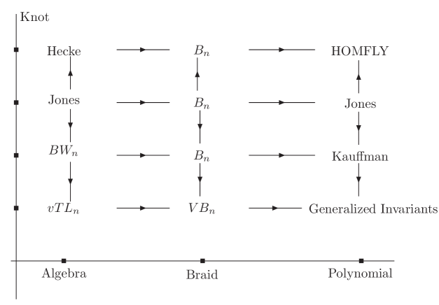
Figure 20: An $ABPK$ diagram showing knot theory

7 Universal quantum gate and unitary braid representation

In terms of identity $Id$, the permutation $P^{\pm}$ and its deformed partial transpose $Q_{\ast}$, we determine a family of unitary braid representation. We recognize these as universal quantum gates and write down the related Schrödinger equation and with it calculate the Markov trace for a link invariant to detect linking numbers.

7.1 Universal quantum gate

A two-qubit gate $G$ is a unitary linear mapping from $V\otimes V$ to $V\otimes V$ where $V$ is a two complex dimensional vector space. A gate $G$ is said to be entangling if there is a vector

$$|\alpha\beta\rangle=|\alpha\rangle\otimes|\beta\rangle\in V\otimes V$$

such that $G|\alpha\beta\rangle$ is not decomposable as a tensor product of two qubits. The Brylinskis prove that a two-qubit gate $G$ is universal iff it is entangling [52]. A pure state $|\psi\rangle$ is separable when

$$|\psi\rangle=\sum^{1}_{i,j=0}a_{ij}|ij\rangle,\qquad|ij\rangle=|i\rangle\otimes|j\rangle,\qquad a_{00}a_{11}\neq a_{01}a_{10}.$$ (90)

The unitary $\check{R}(x)$-matrix acting on the state $|\psi\rangle$ has the form

$$\check{R}|\psi_{pt}\rangle=\sum^{1}_{i,j=0}\sum_{k,l=0}^{1}\check{R}^{kl}_{ij}a_{ij}|kl\rangle=\sum^{1}_{k,l=0}\,b_{kl}|kl\rangle.$$ (91)

If there exists $a_{ij}$ leading to $b_{00}b_{11}=b_{01}b_{10}$, then such the $\check{R}$-matrix can be recognized as a universal quantum gate.

With a new variable $u$, the $\check{R}_{\pm}(u)$-matrix (81) has a simpler form

$$\check{R}_{\pm}(u)=\left(\begin{array}[]{cccc}u&0&0&q\\ 0&1&\pm u&0\\ 0&\pm u&1&0\\ q^{-1}&0&0&u\end{array}\right),\qquad u=t\frac{1-x}{1+x}$$ (92)

which is a unitary matrix for $||q||^{2}=1$ and real $t$, $||x||^{2}=1$, the latter two leading to imaginary $u$, i.e., $u=-\bar{u}$. It determines the coefficients $b^{\pm}_{ij}$ to be

$$\left(\begin{array}[]{c}b^{\pm}_{00}\\ b^{\pm}_{01}\\ b^{\pm}_{10}\\ b^{\pm}_{11}\end{array}\right)=\left(\begin{array}[]{c}u\,\,a_{00}+q\,\,a_{11}\\ a_{01}\,\pm u\,a_{10}\\ \pm u\,\,a_{01}+a_{10}\\ q^{-1}a_{00}+ua_{11}\end{array}\right)$$ (93)

and involved products given by

$$b^{\pm}_{00}b^{\pm}_{11} = (1+u^{2})\,a_{00}a_{11}+u(qa^{2}_{11}+q^{-1}a^{2}_{00}),$$

$$b^{\pm}_{01}b^{\pm}_{10} = (1+u^{2})\,a_{00}a_{11}\pm u(a^{2}_{01}+a^{2}_{10}).$$ (94)

As $u\neq 0$, i.e., $x\neq 1$ and $t\neq 0$, the unitary $\check{R}(x)$-matrix (81) is identified with a universal quantum gate.

7.2 The Hamiltonian and unitary evolution

Before deriving the Hamiltonian, we introduce the algebra of the Pauli matrices. Denote two linear combinations of $\sigma_{x}$ and $\sigma_{y}$ respectively by $\sigma_{n_{1}}$ and $\sigma_{n_{2}}$,

$$\sigma_{n_{1}}=\cos{\frac{\varphi}{2}}\,\,\sigma^{x}+\sin{\frac{\varphi}{2}}\,\,\sigma^{y},\qquad\sigma_{n_{2}}=\cos{\frac{\varphi+\pi}{2}}\,\,\sigma^{x}+\sin{\frac{\varphi+\pi}{2}}\,\,\sigma^{y}$$ (95)

which have the corresponding tensor products,

$$\sigma_{n_{1}}\otimes\sigma_{n_{1}}=\left(\begin{array}[]{cccc}0&0&0&q\\ 0&0&1&0\\ 0&1&0&0\\ q^{-1}&0&0&0\\ \end{array}\right),\,\,\,\,\,\,\sigma_{n_{2}}\otimes\sigma_{n_{2}}=-\left(\begin{array}[]{cccc}0&0&0&q\\ 0&0&-1&0\\ 0&-1&0&0\\ q^{-1}&0&0&0\\ \end{array}\right).$$ (96)

They satisfy the following formulas given by

$$\sigma_{n_{1}}\sigma_{n_{2}} = i\sigma^{z}=-\sigma_{n_{2}}\sigma_{n_{1}},\qquad\sigma_{n_{1}}\sigma_{n_{2}}\otimes\sigma_{n_{1}}\sigma_{n_{2}}=-\sigma^{z}\otimes\sigma^{z},$$

$$\sigma_{n_{1}}\otimes\sigma_{n_{1}} = -\sigma_{n_{2}}\sigma^{z}\otimes\sigma_{n_{2}}\sigma^{z},\qquad\sigma_{n_{2}}\otimes\sigma_{n_{2}}=-\sigma_{n_{1}}\sigma^{z}\otimes\sigma_{n_{1}}\sigma^{z}.$$ (97)

Here the $\check{R}(x)$-matrix (81) involves the normalization factor $\rho$. Choose $t=1$, then $\rho=4$. The $\check{R}_{+}(x)$-matrix (81) has the form of the tensor product of the Pauli matrices,

$$\check{R}_{+}(x) = \frac{1}{2}1\!\!1_{4}-\frac{1}{2}x\sigma^{z}\otimes\sigma^{z}+\frac{1}{2}\sigma_{n_{1}}\otimes\sigma_{n_{1}}-\frac{1}{2}x\sigma_{n_{2}}\otimes\sigma_{n_{2}}$$ (98)

$$= 1\!\!1_{4}-(\frac{1}{2}-\frac{1}{2}\sigma_{n_{1}}\otimes\sigma_{n_{1}})-x\sigma^{z}\otimes\sigma^{z}(\frac{1}{2}-\frac{1}{2}\sigma_{n_{1}}\otimes\sigma_{n_{1}})$$

$$= 1\!\!1_{4}-H_{+}-x\sigma^{z}\otimes\sigma^{z}H_{+}$$

and similarly the $\check{R}_{-}(x)$-matrix (81) has the form

$$\check{R}_{-}(x)=1\!\!1_{4}-H_{-}-x\sigma^{z}\otimes\sigma^{z}H_{-}$$ (99)

where the symbols $H_{+}$ and $H_{-}$ are given by

$$H_{+}=\frac{1}{2}(1\!\!1_{4}-\sigma_{n_{1}}\otimes\sigma_{n_{1}}),\qquad H_{-}=\frac{1}{2}(1\!\!1_{4}+\sigma_{n_{2}}\otimes\sigma_{n_{2}}).$$ (100)

Considering three projectors $H_{\pm}$ and $P_{z}$ which satisfy

$$H_{\pm}^{2}=H_{\pm},\qquad P_{z}^{2}=P_{z},\,\,P_{z}=\frac{1}{2}(1\!\!1_{4}+\sigma^{z}\otimes\sigma^{z}),$$

$$P_{z}H_{\pm}=H_{\pm}P_{z},\qquad(P_{z}H_{\pm})^{2}=P_{z}H_{\pm},$$ (101)

we represent the $\check{R}_{\pm}(x)$-matrix (81) by a unitary exponential function

$$\check{R}_{\pm}(\theta) = 1\!\!1_{4}-H_{\pm}-e^{-i\theta}\sigma^{z}\otimes\sigma^{z}H_{\pm}$$ (102)

$$= (1\!\!1_{4}-H_{\pm}+e^{-i\theta}H_{\pm})(1\!\!1_{4}-P_{z}H_{\pm}-P_{z}H_{\pm})$$

$$= e^{-i\theta H_{\pm}}e^{-i\pi P_{z}H_{\pm}}=e^{-i(\theta+\pi P_{z})H_{\pm}}$$

where a formula for the projector $A$ has been exploited,

$$e^{i\alpha A}=\sum_{n=0}^{\infty}\frac{(i\alpha)^{n}}{n!}A^{n}=1\!\!1_{4}+\sum_{n=1}^{\infty}\frac{(i\alpha)^{n}}{n!}A$$

$$=1\!\!1_{4}-A+\sum_{n=0}^{\infty}\frac{(i\alpha)^{n}}{n!}A=1\!\!1_{4}-A+e^{i\alpha}A.$$ (103)

Let us derive the Hamiltonian to determine the unitary evolution of a unitary quantum gate. Denote the state $\psi$ independent of the time variable $\theta$. Its time evolution $\psi(\theta)$ is specified by the $\check{R}(\theta)$-matrix (81), $\psi(\theta)=\check{R}(\theta)\psi$ which leads to the Schrödinger equation,

$$i\,\frac{\partial\psi(\theta)}{\partial\theta}=H(\theta)\psi(\theta),\qquad H(\theta)=i\frac{\partial\check{R}(\theta)}{\partial\theta}\check{R}^{{\dagger}}(\theta).$$ (104)

Hence the Hamiltonian $H_{\pm}(\theta)$ is the projector $H_{\pm}$ given before. The time evolution operator $U_{\pm}(\theta)$ has the form

$$U_{\pm}(\theta)=e^{-iH_{\pm}\theta}=1\!\!1_{4}-H_{\pm}+e^{-i\theta}H_{\pm}$$ (105)

which can set up the CNOT gate with the help of local unitary transformations or single qubit transformations [16].

7.3 The Markov trace as a link invariant

A basic point of this paper is to recognize nontrivial unitary braid representations as universal quantum gates. When a unitary braid representation can detect a link or knot in topological context, it often also has the power of entangling quantum states. Here we have the unitary $\check{R}_{\pm}(u)$-matrix (92) which is a universal quantum gate at $u\neq 0$. In the following, we calculate the Markov trace which is a link invariant in terms of the $\check{R}_{\pm}(u)$-matrix in order to show that at $u\neq 0$ we are able to detect linking numbers.

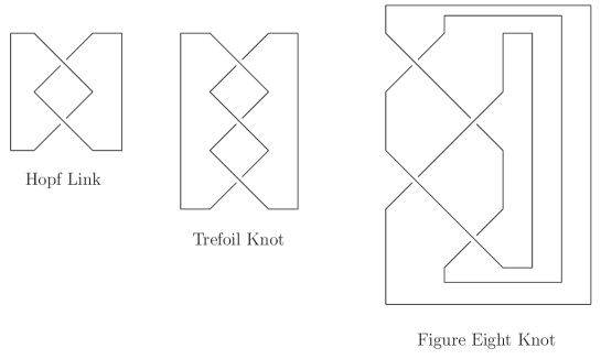
Figure 21: Examples for representing links or knots by the closures of braids

For a given link $L$, the link invariant for the Markov trace has the form

$$Z(L)=\alpha^{-w(b)}Z_{n}(b),\qquad b\in B_{n},\qquad L\sim\bar{b}.$$ (106)

The equivalence relation $L\sim\bar{b}$ says that the link $L$ is isotopic to the closure of a braid $b$, as we are told by the Alexander theorem. For example, the Hopf link, the Trefoil and the Figure Eight knot are represented by the closures of the braids $\sigma_{1}^{2}$, $\sigma_{1}^{3}$ and $\sigma_{1}\sigma_{2}^{-1}\sigma_{1}\sigma_{2}^{-1}$, respectively, see Figure 21. The writhe $w(b)$ of the braid $b$ is the sum of the signs of crossings of the braid $b$. Each under crossing $\sigma_{i}$ and over crossing $\sigma_{i}^{-1}$ contribute $1$ and $-1$ to $w(b)$ respectively. For example, the Hopf link, the Trefoil knot and the Figure Eight knot have the writhe numbers of $2,3,0$, respectively. The normalization factor $\alpha$ is determined by the specific choice of $Z_{n}(b)$ which is well defined on the braid group $B_{n}$ and satisfies the following conditions

$$Z_{n}(gbg^{-1}) = Z_{n}(b),\qquad g,b\in B_{n},$$

$$Z_{n}(b\sigma^{\pm 1}_{n}) = \alpha^{\pm 1}Z_{n}(b),\qquad\sigma_{n}\in B_{n+1},$$ (107)

the second equation also called the Markov move.

Now we set up the Markov trace in terms of the $\check{R}_{\pm}(u)$-matrix (92). To avoid notation ambiguities in this subsection, we denote the $\check{R}_{+}(u)$-matrix by the $\check{R}$-matrix but in fact the $\check{R}_{-}(u)$-matrix leads to the same link invariant. For the generators $\sigma_{i}$ of the braid group $B_{n}$, the representation $\rho_{n}(\sigma_{i})$ has the form

$$\rho_{n}(\sigma_{i})=Id^{\otimes i-1}\otimes\check{R}\otimes Id^{\otimes(n-i-1)},\qquad i=1,\cdots n-1$$ (108)

and thus the Markov trace $Z(L)$ is chosen to be

$$Z(L)=\alpha^{-w(b)}Tr(\rho_{n}(b)).$$ (109)

The normalized factor $\alpha$ is calculated by the partial trace $Tr_{2}(\check{R})$ of the $\check{R}$-matrix,

$$Tr_{2}(\check{R})=\alpha 1\!\!1_{2},\qquad Tr_{2}(\check{R})=\alpha^{-1}1\!\!1_{2}.$$ (110)

The $\check{R}$-matrix has the form

$$\check{R}=\left(\begin{array}[]{cccc}\check{R}^{00}_{00}&\check{R}^{00}_{01}&\check{R}^{00}_{10}&\check{R}^{00}_{11}\\[5.69054pt] \check{R}^{01}_{00}&\check{R}^{01}_{01}&\check{R}^{01}_{10}&\check{R}^{01}_{11}\\[5.69054pt] \check{R}^{10}_{00}&\check{R}^{10}_{01}&\check{R}^{10}_{10}&\check{R}^{10}_{11}\\[5.69054pt] \check{R}^{11}_{00}&\check{R}^{11}_{01}&\check{R}^{11}_{10}&\check{R}^{11}_{11}\end{array}\right),$$ (111)

and its partial trace $Tr_{2}(\check{R})$ is given by

$$Tr_{2}(\check{R}^{ai}_{bj})=\sum_{c=1}^{2}{\check{R}^{ac}_{bc}}=\left(\begin{array}[]{cc}\check{R}^{00}_{00}+\check{R}^{01}_{01}&\check{R}^{00}_{10}+\check{R}^{01}_{11}\\ \check{R}^{10}_{00}+\check{R}^{11}_{01}&\check{R}^{10}_{10}+\check{R}^{11}_{11}\end{array}\right).$$ (112)

If a reader is interested in the detail of the Alexander theorem and the Markov theorem, please consult [1] and [15].

Before computing link invariants, we go through the algebra of $P^{\pm}$, $Q_{\ast}$ given by (51) and $Q^{\ast}=1\!\!1_{4}-Q_{\ast}$. They have the properties

$$(Q^{\ast})^{2n}=(P^{\pm})^{2n}=1\!\!1,\qquad P^{\pm}Q_{\ast}=Q_{\ast}P^{\pm}=Q_{\ast},$$

$$P^{\pm}Q^{\ast}=P^{\pm}(1\!\!1_{4}-Q_{\ast})=P^{\pm}-Q_{\ast}=Q^{\ast}P^{\pm},\qquad n\in{\mathbb{N}}$$ (113)

along with the traces and partial traces of matrices,

$$Tr(P^{\pm})=Tr(Q_{\ast})=2,\qquad Tr(P^{\pm}Q_{\ast})=0,$$

$$Tr_{2}(P^{\pm})=Tr_{2}(Q)_{\ast}=Tr_{2}(Q^{\ast})=1.$$ (114)

With the help of them, we represent the $\check{R}_{\pm}(u)$-matrix (92) in terms of $P^{\pm}$ and $Q^{\ast}$, and derive its inverse given by

$$\check{R}_{\pm}(u)=uP^{\pm}+Q^{\ast},\qquad\check{R}_{\pm}^{-1}(u)=\frac{1}{1-u^{2}}(-uP^{\pm}+Q^{\ast})$$ (115)

which satisfy

$$\check{R}_{\pm}(u)+(1-u^{2})\check{R}_{\pm}^{-1}(u)=2(1\!\!1_{4}-Q_{\ast}),$$ (116)

leading to another normal way of computing a link invariant via the skein relation [1]. The normalization factor $\alpha$ can be fixed by

$$Tr_{2}(\check{R}_{\pm}(u))=1+u,\qquad Tr_{2}(\check{R}^{-1}_{\pm}(u))=\frac{1}{1+u},\qquad\alpha=1+u$$ (117)

As examples, we calculate the Markov traces corresponding to the closures of the braids $\sigma_{1}^{2n}$, $\sigma_{1}^{-2n}$, $\sigma_{1}^{2n+1}$ and $\sigma_{1}^{-2n-1}$ with the writhe number $2n$, $-2n$, $2n+1$ and $-2n-1$, respectively. It is well known that $\overline{\sigma_{1}^{2n}}$ and $\overline{\sigma_{1}^{-2n}}$ are links of two components with the linking numbers $n$ and $-n$. The linking number denotes the half sum of the signs of crossings between two components of a link. Also, $\overline{\sigma_{1}^{2n+1}}$ and $\overline{\sigma_{1}^{-2n-1}}$ are knots for positive number $n$ and they are unknots at $n=0$. The following trace formulas are helpful in calculation,

$$Tr(\check{R}_{\pm}^{2n}) = \sum_{k=0}^{2n}C_{2n}^{k}u^{k}Tr((P^{\pm})^{k}(Q^{\ast})^{2n-k})$$

$$=4\sum_{l=0}^{n}C_{2n}^{2l}u^{2l}=2((1+u)^{2n}+(1-u)^{2n}),$$

$$Tr(\check{R}_{\pm}^{2n+1}) = \sum_{k=0}^{2n+1}C_{2n+1}^{k}u^{k}Tr((P^{\pm})^{k}(Q^{\ast})^{2n+1-k})$$ (118)

$$=2\sum_{k=0}^{2n+1}C_{2n+1}^{k}u^{k}=2(1+u)^{2n+1}$$

where the symbol $C_{n}^{m}$ denotes $n!/m!(n-m)!$. Similarly we have

$$Tr(\check{R}_{\pm}^{-2n})=\frac{2}{(1-u)^{2n}}+\frac{2}{(1+u)^{2n}},\qquad Tr(\check{R}_{\pm}^{-2n-1})=\frac{2}{(1+u)^{2n+1}}.$$ (119)

The Markov traces for the links $\overline{\sigma_{1}^{2n}}$ and $\overline{\sigma_{1}^{-2n}}$ are obtained to be

$$Z(\overline{\sigma_{1}^{2n}}) = (1+u)^{-2n}Tr(\check{R}_{\pm}^{2n})=2(1+{u^{\prime}}^{n}),\qquad u^{\prime}=(\frac{1-u}{1+u})^{2},$$

$$Z(\overline{\sigma_{1}^{-2n}}) = (1+u)^{2n}Tr(\check{R}_{\pm}^{-2n})=2(1+{u^{\prime}}^{-n}),$$ (120)

and the Markov traces for knots $\overline{\sigma_{1}^{2n+1}}$ and $\overline{\sigma_{1}^{-2n-1}}$ are the result given by

$$Z(\overline{\sigma_{1}^{2n+1}})=Z(\overline{\sigma_{1}^{-2n-1}})=2.$$ (121)

They detect linking numbers for links of two components and distinguish links with nonvanishing linking numbers from knots of one component. But they can not classify knots in the examples we are concerned about. In addition, we compute the Markov traces for the Figure Eight knot $\sigma_{1}\sigma_{2}^{-1}\sigma_{1}\sigma_{2}^{-1}$, the Borromean rings $\sigma_{2}\sigma_{1}^{-1}\sigma_{2}\sigma_{1}^{-1}\sigma_{2}\sigma_{1}^{-1}$ and the Whitehead link $\sigma_{1}^{2}\sigma_{2}^{-1}\sigma_{1}\sigma_{2}^{-1}$, which are given by respectively

$$Z(Figure\,\,Eight)=2,\qquad Z(Borromean)=8,\qquad Z(Whitehead)=4.$$ (122)

Note that for simplicity we compute the Markov trace in terms of the $\check{R}_{\pm}(u)$-matrix (92) instead of its normalized unitary form. To conclude this subsection, we remark that when $u=0$ the $\check{R}_{\pm}(u)$-matrix (92) is neither a universal quantum gate nor detects the linking number, as supports the identification of a nontrivial unitary braid representation with a universal quantum gate.

8 Concluding remarks and outlooks

As a concluding remark, Figure 22, a fish diagram represents what we have done in the whole paper under the spell of permutation and its partial transpose. This fish sees a long history, relating the Brauer algebra to the virtual Temperley–Lieb algebra and further to the virtual braid group and finally to YBEs, and relating the commutant of the orthogonal group to the virtual knot theory. She unifies our proposal of the virtual Temperley–Lieb algebra from the viewpoint of the virtual knot theory [24, 25, 26] with the Hecke algebra representation of braid groups and link polynomials [30, 31, 32] into a complete picture.

Figure 22: Fish diagram for the Brauer algebra, $vTL_{n}$ algebra, $VB_{n}$ and $YBEs$.

The permutation $P$ and its partial transpose $P_{\ast}$ appear similar but behave differently. The $P$ and $1\!\!1+uP$ are the simplest examples for YBE solutions but $1\!\!1+uP$ does not form a braid representation. The permutation’s partial transpose $P_{\ast}$ is an idempotent of the $TL$ algebra and the $1\!\!1+vP_{\ast}$ can form a braid representation. It is worthwhile emphasizing that the Werner state has the form of $1\!\!1+uP$ and the isotropic state has $1\!\!1+vP_{\ast}$. The YBE in terms of matrix entries is a set of highly non-linear equations. Its solutions are difficult to obtain unless enough constraints are imposed. Common solutions of the braid relation (5), the multiplicative YBE (14) and additive YBE (15) are found by exploring the linear combinations of $Id$, $P$ and $P_{\ast}$. It is surprising because it satisfies three quite different highly non-linear equations and roots in the existence of flat unrestricted braid representations $FU_{2}$ of $P$ and $P^{\ast}$.

The partial transpose [4, 5] plays important roles in quantum information theory. Our research is expected to be helpful in topics such as Bell inequalities [7], quantum entanglement measures [12] and quantum data hiding [14]. We will apply topological contents of a family of unitary braid representations to universal quantum gates and quantum entanglement measures. Besides that, we set up new quantum algebras [37] from eight-vertex models [16, 17] with the help of projectors of $P$ and $P_{\ast}$. In the paper, we articulate the concepts of the $PPT_{n}$ algebra and virtual Temperley–Lieb algebras. The $PPT$ algebra underlies the construction of multipartite symmetric states [13] and plays crucial roles in detecting separable quantum states [12] and making quantum data hiding [14].

The family of virtual braid representations set up representations for the family of the virtual knot theory. The point about the virtual knot theory is that by adding a permutation to the braiding theory we actually bring the structure closer to quantum information theory where the permutation (swap gate) is very important. Once one has the swap gate one only needs to add a simple phase gate like $Diag(1,1,1,-1)$ to obtain universality (in the presence of $U(2)$). So it is certainly interesting to have these solutions. The $\check{R}_{\pm}$-matrices (75) or (81) are universal quantum gates, see [16, 17] for details.

Note that in [62] we study the applications of the $TL$ algebra, Brauer algebra or virtual $TL$ algebra to quantum teleportation phenomena. We find that the $TL$ algebra under local unitary transformations underlies quantum information protocols involving maximally entangled states, projective measurements and local unitary transformations. We propose that the virtual braid group is a natural language for the quantum teleportation. Especially, we realize the teleportation configuration to be a basic element of the Brauer algebra or virtual $TL$ algebra.

Appendix A The Hecke algebra representation of the braid group

The Hecke algebra $H_{n}$ of Type $A$ is generated by $1\!\!1$ and $n-1$ hermitian projections $e_{i}$ satisfying

$$e_{i}^{2} = e_{i},\qquad(e_{i})^{\dagger}=e_{i},\,\,\,i=1,\ldots,n-1,$$

$$e_{i}e_{i+1}e_{i}-\lambda e_{i} = e_{i+1}e_{i}e_{i+1}-\lambda e_{i+1},\qquad e_{i}e_{j}=e_{j}e_{i},\,\,\,|i-j|>1.$$ (123)

The parameter $\lambda$, which clearly must be in the interval $[0,1]$ if we want a $\ast$-representation on a Hilbert space, is fixed. Just to get three formulas used in the following, observe that for a pair of projections $p,q$, and a real number $0<\lambda<1$ the following are equivalent:

$$(1)\,\,pqp=\lambda p,\qquad(2)\,\,[q,pqp-\lambda p]=0,\qquad(3)\,\,pqp-\lambda p=qpq-\lambda q.$$ (124)

Proof: The turbo version is to appeal to the universal C*-algebra generated by two projections. (3)$\Rightarrow$(2), because the RHS commutes with $q$. Now (2) implies that $x=pqp-\lambda p$ is in the center of the C*-algebra generated by $p,q$. Consider any irreducible representation, in which $x$ is then a scalar. But $xp=x$, and hence $x\neq 0$ implies $p=1$, which implies $q=\lambda$, which is not a projection. It follows that $x=0$ in every irreducible representation, which is (1). Finally, assuming (1), we get (2) with the roles of $p,q$ interchanged $(qpq-\lambda q)p=q(pqp-\lambda p)$. Hence by the argument for (2)$\Rightarrow$(1) just given, both vanish.

$\hfill\Box$

Now fix $\alpha\neq\beta\in{\bf C}$, set

$$\sigma_{j}=\alpha e_{j}+\beta(1-e_{j}),$$

and ask, when these operators satisfy braid relations. Then, only using $e_{i}^{2}=e_{i}$, but not the $TL$ relation, we get

$$\sigma_{j}\sigma_{j+1}\sigma_{j}-\sigma_{j+1}\sigma_{j}\sigma_{j+1} = \alpha\beta(\alpha-\beta)(e_{j}-e_{j+1})$$ (125)

$$\quad+(\alpha-\beta)^{3}(e_{j}e_{j+1}e_{j}-e_{j+1}e_{j}e_{j+1})$$

where the terms $e_{j}e_{j+1}$ cancel. Hence by the equivalence (3)$\Leftrightarrow$(1), the braid relations are satisfied for the $\sigma_{i}$, iff the $e_{i}$ satisfy the Hecke algebra of type $A$ with

$$\lambda=\frac{-\alpha\beta}{(\alpha-\beta)^{2}}.$$ (126)

Note that since the braid relation is homogenous, the expression for $\lambda$ does not depend on a common factor of $\alpha$ and $\beta$. Exchanging the two eigenvalues of $\sigma_{i}$ gives the inverse (up to a factor), which again satisfies braid relations. Hence the expression for $\lambda$ is symmetric in $\alpha$ and $\beta$. Moreover, given $\lambda$, we can solve a quadratic equation for $(\alpha/\beta)$.

Suppose $\alpha,\beta$ have the same modulus, which is equivalent to saying that $\sigma_{i}$ is unitary up to a factor. Then by choosing the factor we may set $\alpha=\exp(it)$, $\beta=\exp(-it)$, with $0\leq t\leq\pi/2$, which produces $\lambda=1/(2\sin t)^{2}$. Note that we cannot choose $t\approx 0$, or, more precisely, we need $\sin t>1/2$, so that the eigenvalues of a unitary braid group generator must be at least $\pi/3$ apart. At the extreme other end ($t=\pi/2\Leftrightarrow\lambda=1/4$), we can write the eigenvalues as $\pm 1$, so that we effectively have a representation of the permutation group, rather than the braid group. In the regime $\lambda<1/4$ we can choose both eigenvalues $\alpha,\beta$ real, hence $\sigma_{i}^{*}=\sigma_{i}$. Clearly this is what happens in the paper. Note that $e_{i}=\frac{1}{d}P_{*}$ satisfies the $TL_{2}$ algebra with $\lambda=d^{-2}$, namely $d^{3}(e_{j}e_{j+1}e_{j})=de_{j}$ and $d^{2}e_{j}^{2}=d\cdot de_{j}$. Then the parameters $v_{\pm}$ (25) for fixing the braid generator correspond to the $\alpha,\beta$ satisfying (126).

Note on the Jones–Wenzl representation [30, 31, 32, 59]: Its parameter $\lambda$ denotes the quantum factorial $[2]$ given by

$$\lambda=[2]^{-2},\qquad[2]=-q^{2}-q^{-2}=-2\cos\frac{\pi}{r},\,\,q=\exp(\pi i/{2r}),\,\,r\geq 3.$$ (127)

The number “2” in brackets refers to $SU(2)$, while the general $SU(k)$ theory with $r\geq k+1$ gives rise to the HOMFLY polynomial [54, 60, 61]. Here we have

$$d=-q^{2}-q^{-2},\qquad q=\pm\frac{1}{2}i\sqrt{d\mp\sqrt{d^{2}-4}}.$$ (128)

As $r\to\infty$ and $q\to 1$, we obtain $d=2$ so that our projector is a kind of limit of the Jones–Wenzl projector.

Appendix B The proof at $d>2$ for Theorem 1

At $d>2$ and $a\neq 0$, Theorem 1 remarks that the $\check{R}(u)$ operator (69) does not satisfy the braid relation (5) and is not a solution of the YBE (14) or (15) with the coefficient of $P$ as the spectral parameter. As an example, we prove that the $\check{R}(u)$ operator (69) does not satisfy the YBE (15) for $d>2,a\neq 0$. The remaining two statements are verified in a similar way. The left handside of the YBE (15) acts on the basis $|ijk\rangle$ in the way

$$(\check{R}(u)\otimes Id)\,(Id\otimes\check{R}(u+v))\,(\check{R}(v)\otimes Id)|ijk\rangle$$ (129)

$$= (a^{3}+uav)|ijk\rangle+(a^{2}v+ua^{2})|jik\rangle$$

$$+(uab+2ba^{2}+bav+b^{2}ad+b^{2}(u+v)+b^{3})\sum_{l=1}^{d}|llk\rangle\delta_{ij}$$

$$+a^{2}(u+v)|ikj\rangle+av(u+v)|jki\rangle+(b(u+v)a+b^{2}u)\sum_{l=1}^{d}|lkl\rangle\delta_{ij}$$

$$+ba^{2}\sum_{l=1}^{d}|ill\rangle\delta_{jk}+avb\sum_{l=1}^{d}|jll\rangle\delta_{ik}+(b^{2}a+bu(u+v))\sum^{d}_{l,m=1}|kll\rangle\delta_{ij}$$

$$+ua(u+v)|kij\rangle+uv(u+v)|kji\rangle+uba\sum_{l=1}^{d}|lil\rangle\delta_{jk}+uvb\sum_{l=1}^{d}|ljl\rangle\delta_{ik}$$

$$+(ba(u+v)+b^{2}v)\sum_{l=1}^{d}|llj\rangle\delta_{ik}+(bv(u+v)+ab^{2})\sum_{l=1}^{d}|lli\rangle\delta_{jk},$$

while the action of the right handside of the YBE (15) on $|ijk\rangle$ has the form

$$(Id\otimes\check{R}(v))\,(\check{R}(u+v)\otimes Id)\,(Id\otimes\check{R}(u))|ijk\rangle$$ (130)

$$= (a^{3}+auv)|ijk\rangle+a^{2}(u+v)|jik\rangle+uv(u+v)|kji\rangle+au(u+v)|kij\rangle$$

$$+(ab(u+v)+b^{2}v)\sum_{l=1}^{d}|lil\rangle\delta_{jk}+a^{2}b\sum_{l}^{d}|llk\rangle\delta_{ij}+(ab^{2}+b(u+v)v)\sum_{l=1}^{d}|lli\rangle\delta_{jk}$$

$$+a(u+v)v|jki\rangle+(abv+abu+b^{2}(u+v)+b^{3}+2a^{2}b+ab^{2}d)\sum_{l=1}^{d}|ill\rangle\delta_{jk}$$

$$+a^{2}(u+v)|ikj\rangle+abv\sum_{l}^{d}|lkl\rangle\delta_{ij}+(ab(u+v)+ub^{2})\sum_{l=1}^{d}|jll\rangle\delta_{ki}$$

$$+(ab^{2}+ub(u+v))\sum_{l=1}^{d}|kll\rangle\delta_{ij}+uab\sum_{l=1}^{d}|llj\rangle\delta_{ki}+uvb\sum_{l=1}^{d}|ljl\rangle\delta_{ki}.$$

On both sides, there are $15$ terms independent of each other. The dimension of the vector space of the three-fold tensor product is $d^{3}$. If $d>2$ then $d^{3}>15$, we are allowed to recognize every term on both sides and obtain three equations of $a,b,d$ given by

$$\left\{\begin{array}[]{cll}abu&=&ab(u+v)+b^{2}v,\\ abv&=&ab(u+v)+b^{2}u,\\ a^{2}b&=&ab(u+v)+b^{2}(u+v)+b^{3}+2a^{2}b+ab^{2}d.\end{array}\right.$$ (131)

At $a\neq 0$ and $u,v$ as constants, there is a unique solution: $d=2,a=-b$, supporting the statement that the $\check{R}(u)$-matrix (71) satisfies the YBE (15).

References

- [1] L.H. Kauffman, Knots and Physics (World Scientific Publishers, 2002).
- [2] M. Nielsen and I. Chuang, Quantum Computation and Quantum Information (Cambridge University Press, 1999).
- [3] M.M. Wolf, Partial Transposition in Quantum Information Theory, PhD. Thesis (TU Braunschweig, 2003).
- [4] A. Peres, Separability Criterion for Density Matrices, Phys. Rev. Lett. 77 (1996) 1413-1415. Arxiv: quant-ph/9604005.
- [5] M. Horodecki, P. Horodecki and R. Horodecki, Separability of Mixed States: Necessary and Sufficient Conditions, Phys. Lett. A 223 (1996) 1. Arxiv: quant-ph/9605038.
- [6] R.F. Werner, Quantum Information Theory–An Introduction to Basic Theoretical Concepts and Experiments, Chapter Quantum Information Theory–An Invitation (Springer–Verlag, New York, 2001).
- [7] R.F. Werner, Quantum States with Einstein-Podolsky-Rosen Correlations Admitting a Hidden-Variable Model, Phys. Rev. A 40 (1989) 4277.
- [8] C.N. Yang, Some Exact Results for the Many Body Problems in One Dimension with Repulsive Delta Function Interaction, Phys. Rev. Lett. 19 (1967) 1312-1314.
- [9] R.J. Baxter, Partition Function of the Eight-Vertex Lattice Model, Annals Phys. 70 (1972) 193-228.
- [10] M. Horodecki and P. Horodecki, Reduction Criterion of Separability and Limits for A Class of Distillation Protoco, Phys. Rev. A 59 (1999) 4206.
- [11] R. Brauer, On Algebras Which Are Connected With the Semisimple Continuous Groups, Ann. of Math. 38 (1937) 857-872.
- [12] K.G. H. Vollbrecht and R.F. Werner, Entanglement Measures under Symmetry, Phys. Rev. A 64 (2001). Arxiv: quant-ph/0010095.
- [13] T. Eggeling, On Multipartite Symmetric States in Quantum Information Theory, PhD. Thesis (TU Braunschweig, 2003).
- [14] T. Eggeling and R.F. Werner, Hiding Classical Data in Multi-Partite Quantum States, Phys. Rev. Lett. 89 (2002). Arxiv: quant-ph/0203004.
- [15] L.H. Kauffman and S.J. Lomonaco Jr., Braiding Operators are Universal Quantum Gates, New J. Phys. 6 (2004) 134. Arxiv: quant-ph/0401090.
- [16] Y. Zhang, L.H. Kauffman and M.L. Ge, Universal Quantum Gate, Yang–Baxterization and Hamiltonian. Int. J. Quant. Inform., Vol. 3, 4 (2005) 669-678. Arxiv: quant-ph/0412095.
- [17] Y. Zhang, L.H. Kauffman and M.L. Ge, Yang–Baxterizations, Universal Quantum Gates and Hamiltonians. Quant. Inf. Proc. 4 (2005) 159-197. Arxiv: quant-ph/0502015.
- [18] L.H. Kauffman, Quantum Computation and the Jones Polynomial, in Quantum Computation and Information, S. Lomonaco, Jr. (ed.), AMS CONM/305, 2002, pp. 101-137. Arxiv: math. QA/0105255.
- [19] L.H. Kauffman, Quantum Topology and Quantum Computing, in Quantum Computation, S. Lomonaco (ed.), AMS PSAPM/58, 2002, pp. 273–303.
- [20] L. H. Kauffman and S. J. Lomonaco Jr., Quantum Knots, in E. Donkor, A.R. Pirich and H.E. Brandt (eds.), Quantum Information and Computation II, Spie Proceedings, (12 -14 April, Orlando, FL, 2004), Vol. 5436, pp. 268-284. Arxiv: quant-ph/0403228.
- [21] L.H. Kauffman and S.J. Lomonaco Jr., Quantum Entanglement and Topological Entanglement, New J. Phys. 4 (2002) 73.1–73.18.
- [22] L.H. Kauffman and S.J. Lomonaco Jr., Entanglement Criteria–Quantum and Topological, in E. Donkor, A.R. Pirich and H.E. Brandt (eds.), Quantum Information and Computation – Spie Proceedings, (21-22 April, Orlando, FL, 2003), Vol. 5105, pp. 51-58. Arxiv: quan-ph/0304091.
- [23] L.H. Kauffman, Teleportation Topology. Opt. Spectrosc. 9 (2005) 227-232. Arxiv: quan-ph/0407224.
- [24] L.H. Kauffman, Virtual Knot Theory, European J. Comb. 20 (1999) 663-690.
- [25] L. H. Kauffman, A Survey of Virtual Knot Theory, in “Proceedings of Knots in Hellas 98” (World Scientific, Singpore, 2000) 143-202.
- [26] L. H. Kauffman, Detecting Virtual Knots, Atti. Sem. Mat. Fis. Univ. Modena, Supplemento al Vol. IL (2001) 241-282.
- [27] S. Kamada, Braid Representation of Virtual Knots and Welded Knots, Arxiv: math. GT/0008092.
- [28] H.N.V. Temperley and E.H. Lieb, Relations between the ‘Percolation’ and ‘Colouring’ Problem and Other Graph-Theoretical Problems Associated with Regular Planar Lattices: Some Exact Results for the ‘Percolation’ Problem, Proc. Roy. Soc. A 322 (1971) 251-280.
- [29] L.H. Kauffman and S.L. Lin, Temperley–Lieb Recoupling Theory and Invariants of Three-Manifold, Ann. of Math. Stud. 114 (Princeton Univ. Press, 1994).
- [30] V.F.R. Jones, Heck Algebra Representations of Braid Groups and Link Polynomials, Ann. of Math. 126 (1987) 335-388.
- [31] V.F.R. Jones, Braid Groups, Heck Algebra and Type II Factors, Geometric Methods in Abstract Algebras, Proc. U.S.-Japan Symposium (Wiley, 1986) 242-273.
- [32] V.F.R. Jones, A Polynomial Invariant for Knots via Von Neuman Algebras, Bull. Amer. Math. Soc. (N.S.) 12 (1985) 103-111.
- [33] V.F.R. Jones, Baxterization, Int. J. Mod. Phys. A 6 (1991) 2035-2043.
- [34] J. Murakami, A State Model for the Multi-Variable Alexander Polynomial, Talk at Int. Workshop on Quantum Group (Euler International Mathematical Institute, Leninggrad, 1990).
- [35] M.L. Ge and K. Xue, Trigonometric Yang–Baxterization of Coloured -matrix, J. Phys. A: Math Gen. 26 (1993) 281-291.
- [36] H.A. Dye and L.H. Kauffman, Virtual Knot Diagrams and the Witten-Reshetikhin-Turaev Invariant, Arxiv: math. GT/0407407.
- [37] Y. Zhang, N.H. Jing and M.L. Ge, New Quantum Algebras via RRT Relation on Eight–Vertex Models, (in preparation).
- [38] F.Y. Wu, The Potts Model, Rev. Mod. Phys. 54 (1982) 235-68.
- [39] F.Y. Wu, Knot Theory and Statistical Mechanics, Rev. Mod. Phys. 64 (1992) 1099-1131.
- [40] L.H. Kauffman, State Model for the Jones Polynomial, Topology 26 (1987) 395-407.
-
[41]
P.P. Kulish, On Spin Systems Related to the Temperley–Lieb Algebra,
J. Phys. A: Math. Gen. 36 (2003) L489-L493. - [42] J. Birman and H. Wenzl, Braids, Link Polynomials and a New Algebra, Trans. Amer. Math. Soc. 313 (1989) 249-273.
- [43] J. Murakami, The Kauffman Polynomial of Links and Representation Theory, Osaka J. Math. 24 (1987) 745-758.
- [44] R. Fenn, R. Rimanyi, C. Rourke, The Braid Permutation Group, Topology 36 (1997) 123–135.
- [45] T. Kanenobu, Forbidden Moves Unknot a Virtual Knot, J. Knot Theory and Its Ramifications 10 (2001) 89–96.
- [46] S. Nelson, Unknotting Virtual Knots With Gauss Diagram Forbidden moves, J. Knot Theory and Its Ramifications 10 (2001) 931–935.
- [47] L.H. Kauffman and S. Lambropoulou, Virtual Braids, Fund. Math. 184 (2004) 159-186. ArXiv: math.GT/0407349.
- [48] M.L. Ge, L. H. Gwa and H. K. Zhao, Yang–Baxterization of the Eight-Vertex Model: the Braid Group Approach, J. Phys. A: Math. Gen. 23 (1990) L 795-L 798.
- [49] H. Wenzl, Representations of Heck Algebra and Subfactors, PhD. Thesis (University of Pennsylvania, 1985).
- [50] H. Wenzl, Heck Algebras of Type A and Subfactors, Invent. Math. 92 (1988) 173-193.
- [51] H.A. Dye, Unitary Solutions to the Yang–Baxter Equation in Dimension Four, Quant. Inf. Proc. 2 (2003) 117-150. Arxiv: quant-ph/0211050.
- [52] J.L. Brylinski and R. Brylinski, Universal Quantum Gates, in Mathematics of Quantum Computation, Chapman & Hall/CRC Press, Boca Raton, Florida, 2002 (edited by R. Brylinski and G. Chen).
- [53] L.H. Kauffman, Knot Diagrammatics, in W. Menasco and M. Thistlethwaite (eds.), Handbook of Knot Theory, (Elsevier, 2005), pp. 233–318. Arxiv: math. GN/0410329.
- [54] P. Freyd, D. Yetter, J. Hoste, W.B.R. Lickorish, K. Miller, and A. Ocneanu, A New Polynomial Invariant of Knots and Links, Bull. Amer. Math. Soc. (N.S.) 12 (1985) 239-246.
- [55] L.H. Kauffman, An Invariant of Regular Isotopy, Trans. Amer. Math. Monthly 95 (1988) 195-242.
- [56] H.A. Dye and L.H. Kauffman, Minimal Surface Representations of Virtual Knots and Links, Arxiv: math. GT/0401035.
- [57] V.O. Manture, Kauffman-Like Polynomial and Curve in 2-Surfaces, J. Knot Theory and Its Ramifications 12 (2003) 1145-1153.
- [58] H. Wenzl, On the Structure of Brauer’s Centralized Algebras, Ann. of Math. 128 (1988) 179-193.
- [59] H. Wenzl, On Sequences of Projections, C. R. Math. Acad. Sci. Soc. R. Can. 9 (1987) 5-9.
- [60] M.H. Freedman, M.J. Larsen and Z. Wang, The Two-Eigenvalue Problem and Density of Jones Representation of Braid Groups, Comm. Math. Phys. 228 (2002) 177-199.
- [61] S. Reznikoff, Representations of the Temperley–Lieb Planar Algebra, PhD. Thesis (University of California, Berkeley, 2002).
- [62] Y. Zhang, Teleportation, Braid Group and Temperleyt–Lieb algebra, Arxiv: quant-ph/0601050.