Engineering multiphoton states for linear optics computation

Abstract

Transformations achievable by linear optical components allow to generate the whole unitary group only when restricted to the one-photon subspace of a multimode Fock space. In this paper, we address the more general problem of encoding quantum information by multiphoton states, and elaborating it via ancillary extensions, linear optical passive devices and photodetection. Our scheme stems in a natural way from the mathematical structures underlying the physics of linear optical passive devices. In particular, we analyze an economical procedure for mapping a fiducial 2-photon 2-mode state into an arbitrary 2-photon 2-mode state using ancillary resources and linear optical passive $N$-ports assisted by post-selection. We found that adding a single ancilla mode is enough to generate any desired target state. The effect of imperfect photodetection in post-selection is considered and a simple trade-off between success probability and fidelity is derived.

1 Introduction

A quantum computer N-C , although still a chimera as a concrete device, is already a venerable object for physicists, mathematicians and computer scientists, for the wide range of completely new perspectives that such a tool should offer for the development of science as well as for technological applications.

Photon states are stable against decoherence, and are currently produced and manipulated in modern laboratories. These features make the possibility of implementing quantum logic gates particularly attractive. One of the most promising architectures for implementing a quantum computer by means of optical systems is based on a scheme proposed by Knill, Laflamme and Milburn (KLM) KLM . In this scheme, information is encoded by (tensor products of) single-photon two-mode states of the quantized e.m. field; precisely, the qubit states are identified with a couple of single-photon states on two optical modes (dual rail logic) and multi-qubits are obtained by tensor products. The basic ingredients for the elaboration of information in the KLM scheme are linear optical passive (LOP) components review — essentially, phase shifters and beam splitters — by which one is able to realize the single qubit gates; all other operations can be obtained in a non-deterministic way exploiting, in addition, ancillary optical modes and photodetection. One can show that, with the KLM scheme — hence, using only single photon sources, LOP devices and photodetectors — it is possible to simulate efficiently, i.e. by means of a polynomial amount of resources, an ideal quantum computer review_1 ; review_2 .

It is worth noting, however, that in the KLM scheme, states that are not in the dual rail logic (e.g. the state $|2000\rangle$) may be produced during the computation process, even if at the output they recombine to get back to the dual rail encoding. As it will be shown in the following, this is a consequence of the fact that the linear space spanned by all $n$-photon states (on a given number $N$ of optical modes) is the carrier Hilbert space of an irreducible unitary representation of $\mathrm{U}(N)$ which is associated in a natural way with the action of LOP devices. It seems then quite natural to investigate, in addition to the KLM dual rail logic, also the possibility of encoding information by means of $n$-photon $N$-mode states, with $n\geq 1$ and $N\geq 2$. The case where $n=1$ and $N\geq 2$, with gates implemented only by LOP components, has been considered by Cerf et al. Cerf . This scheme is easily seen to be not scalable.

In this paper, we will consider the case where information is encoded by $n$-photon states, with $n>1$, on $N\geq 2$ modes and logic gates are obtained by LOP components and photodetectors. As anticipated, this scheme stems in a natural way from the mathematical structures underlying the physics of LOP devices, structure that has been investigated in two previous papers P-R ; future . We will now address, as a first step, the following problem: to engineer any desired state — which may be regarded as the ‘input state’ of a quantum computation process — in the chosen encoding space, starting with a fixed ‘fiducial state’, namely, a photon state that can be easily produced by single-photon sources. For the sake of definiteness, we will focus on the case where $n=N=2$. This is the simplest case that is not contemplated in the Cerf et al. and in the KLM schemes. Notice that in our case the building blocks of quantum information are qutrits instead of qubits.

The paper is structured as follows. In Section 2, the basic mathematical ingredients for a natural and systematic description of LOP transformations are recalled. Next, in Sections 3 and 4, our encoding and elaboration scheme is presented. The effect of realistic imperfect photodetection is then discussed in Section 5. Finally, in Section 6, we end up with some concluding remarks.

2 A group theoretical approach to LOP components

A generic LOP transformation can be described as a $2N-$port, namely a black box with $N$ input modes and $N$ output modes. A pictorial representation is given in figure 1. In two previous papers P-R ; future , it has been shown that the natural mathematical description of the action of LOP transformations is based on the theory of representations of semi-simple Lie groups and algebras; in this framework a special role is played by the Jordan-Schwinger map JSmap ; JSmap_1 . In this section, we recall the basic ingredients of such a description.

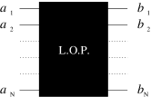
Figure 1: a black-box picture of a $2N-$port based on L.O.P. transformation

Let us consider a set of $N$ optical modes with the associated field operators

$$a_{i},a_{i}^{\dagger}\ \ \ \ i=1,2\ldots N,$$ (1)

where the index $i$ may label both spatial or polarization modes of the field, with the canonical commutation relations

$$[a_{i},a_{j}^{\dagger}]=\delta_{ij}{\mathbbm{I}},\ \ \ \ [a_{i},a_{j}]=[a_{i}^{\dagger},a_{j}^{\dagger}]=0,$$ (2)

where ${\mathbbm{I}}$ is identity operator. It is well known that the set of operators $\{a_{i},a_{i}^{\dagger},{\mathbbm{I}}\}$, endowed with the canonical commutation relations (2), are the generators of a realization of the $N-$dimensional Heisenberg-Weyl algebra $\mathcal{W}(N)$ P-R . We indicate with $\mathcal{H}^{(N)}$ the bosonic Fock space associated with the chosen set of $N$ modes.

We are interested in Linear Optical Passive (LOP) transformations, i.e., maps that are linear in the field amplitudes

$$\left\{\begin{array}[]{ccc}a_{i}&\longrightarrow&b_{i}=M_{ij}a_{j}+N_{ij}a_{j}^{\dagger}\\ a_{i}^{\dagger}&\longrightarrow&b_{i}^{\dagger}=M_{ij}^{*}a_{j}^{\dagger}+N_{ij}^{*}a_{j}\end{array}\right.$$ (5)

(where the sum over repeated indices is assumed) and preserve the total photon number operator

$$\sum_{i=1,\ldots N}b_{i}^{\dagger}b_{i}=\sum_{i=1,\ldots N}a_{i}^{\dagger}a_{i}.$$ (6)

It is easy to show that the only maps with properties (5-6) are of the form:

$$\left\{\begin{array}[]{ccc}a_{i}&\longrightarrow&b_{i}=M_{ij}a_{j}\\ a_{i}^{\dagger}&\longrightarrow&b_{i}^{\dagger}=M^{*}_{ij}a_{j}^{\dagger}\end{array}\right.$$ (9)

where $M_{ij}$ is a $N\times N$ unitary matrix ($M\in\mathrm{U}(N)$). It is also a simple calculation to verify that a map of the form (9) preserves the canonical commutation relations:

$$[b_{i},b_{j}^{\dagger}]=[a_{i},a_{j}^{\dagger}]=\delta_{ij}{\mathbbm{I}},$$ (10)

$$[b_{i},b_{j}]=[b_{i}^{\dagger},b_{j}^{\dagger}]=[a_{i},a_{j}]=[a_{i}^{\dagger},a_{j}^{\dagger}]=0.$$ (11)

Thus one can consider the two realizations of the ($N$ dimensional) Heisenberg-Weyl algebra given by $\{a_{i},a_{i}^{\dagger},{\mathbbm{I}}\}$ and $\{b_{i},b_{i}^{\dagger},{\mathbbm{I}}\}$ and notice that by virtue of the Stone-von Neumann theorem Stone ; vonN they are unitarily equivalent, that is, it exists an unitary operator $U$ acting in the $N-$modes Fock space such that

$$\left\{\begin{array}[]{ccc}b_{i}&=&U^{\dagger}a_{i}U\\ b_{i}^{\dagger}&=&U^{\dagger}a_{i}^{\dagger}U\end{array}\right.$$ (14)

Notice that the operator $U$ is defined only up to an arbitrary phase factor. Since by construction $U$ commutes with the total photon number operator this phase factor is fixed by the action of $U$ on the vacuum state:

$$U|0\rangle=e^{i\phi(U)}|0\rangle.$$ (15)

This ambiguity can be removed if one considers an explicit construction of the unitary operator $U$. This can be done by means of the Jordan-Schwinger map.

2.1 The Jordan-Schwinger map

The Jordan-Schwinger (JS) map JSmap ; JSmap_1 , in its general formulation, maps a Lie algebra into an algebra of operators defined on a bosonic Fock space, this map being an algebra homomorphism. The JS map is defined as follows. Let us consider a $m-$dimensional Lie algebra realized as an algebra of $N\times N$ matrices with a given basis of generators

$$Q^{(\alpha)}\equiv||Q^{(\alpha)}_{ij}||\ \ \ \ \alpha=1,2,\ldots m\ \ i,j=1,2,\ldots N$$ (16)

and commutation relations

$$[Q^{(\alpha)},Q^{(\beta)}]=c^{\alpha\beta}_{\gamma}Q^{(\gamma)}.$$ (17)

Let us also consider a $N-$mode bosonic Fock space with field operators $a_{i},a_{i}^{\dagger}\ \ i=1,2,\ldots N$ and the (normal ordered) operators

$$d_{ij}=a_{i}^{\dagger}a_{j}.$$ (18)

The operators (18) satisfy the following commutation relations:

$$[d_{ij},d_{hk}]=d_{ik}\delta_{hj}-d_{hj}\delta_{ik}.$$ (19)

One can consider the following set of bosonic operators:

$$JS(Q^{(\alpha)})=Q^{(\alpha)}_{ij}d_{ij}.$$ (20)

The map defined on the basis (16)

$$Q^{(\alpha)}\longrightarrow JS(Q^{(\alpha)})=Q^{(\alpha)}_{ij}d_{ij}\;,$$ (21)

extended by linearity, defines the JS map. It is easy to show that by virtue of the commutation relations (19) the JS map is indeed an algebra homomorphism, namely

$$[JS(Q^{(\alpha)}),JS(Q^{(\beta)})]=c^{\alpha\beta}_{\gamma}JS(Q^{(\gamma)}).$$ (22)

Let us now come back to the transformation (14). The $N\times N$ unitary matrix $M$ can be written in terms of the exponential map as $M=\mbox{exp}(A)$, where $A$ is an element of the Lie algebra of the $N-$dimensional unitary group (namely a $N\times N$ anti-hermitian matrix). It is found that the related unitary operator $U$ can be written in the following way by exploiting the JS and the exponential map, namely

$$U=\mbox{exp}(JS(A)).$$ (23)

In order to check this, consider that, for $\epsilon<<1$, we have:

$$U^{\dagger}a_{k}U =\mbox{exp}(-\epsilon JS(A))a_{k}\mbox{exp}(\epsilon JS(A))$$

$$\sim a_{k}+\epsilon[a_{k},JS(A)]$$ (24)

where

$$[a_{k},JS(A)] =A_{ij}\left(a_{k}a_{i}^{\dagger}a_{j}-a_{i}^{\dagger}a_{j}a_{k}\right)$$

$$=A_{ij}\left((a_{i}^{\dagger}a_{k}+\delta_{ik})a_{j}-a_{i}^{\dagger}a_{j}a_{k}\right)=A_{kj}a_{j}.$$ (25)

The JS map allows to fix the arbitrary phase factor in (15). In fact, since the $JS(A)$ is a normally ordered operator, we have:

$$\mbox{exp}(JS(A))|0\rangle=|0\rangle,$$ (26)

so that $e^{i\phi(U)}=1$.

To summarize we have shown that LOP transformations on $N$ modes are described by means of the $N-$dimensional unitary group acting on field operators as in (9). Such an action of the $N-$dimensional unitary group induces a bosonic representation of the group $\mathrm{U}(N)$ acting on the $N$ modes bosonic Fock space

$$U=\Upsilon^{(N)}(M)$$ (27)

that can be explicitly defined by means of the JS map. Indeed it is easy to check that

$$\Upsilon^{(N)}(M_{1}M_{2})=\Upsilon^{(N)}(M_{1})\Upsilon^{(N)}(M_{2}).$$ (28)

Since, by construction, $\Upsilon^{(N)}(M)$ commutes with the total photon number operator, the unitary representation $\Upsilon^{(N)}$ can be written as the direct sum of unitary (sub) representations acting on the subspaces with fixed photon number

$$\Upsilon^{(N)}=\bigoplus_{n=0,1,\ldots\infty}\Upsilon^{(N)}_{n},$$ (29)

in correspondence with the decomposition

$$\mathcal{H}^{(N)}=\bigoplus_{n=0,1,\ldots\infty}\mathcal{H}^{(N)}_{n},$$ (30)

where $\mathcal{H}^{(N)}_{n}$ is the subspace with $n$ photons on $N$ optical modes. A simple calculation shows that the following relation holds:

$$\mbox{dim}\mathcal{H}^{(N)}_{n}=\frac{(n+N-1)!}{n!(N-1)!}.$$ (31)

Hence, the subspace $\mathcal{H}^{(N)}_{n}$ can be seen as the space of a qu-$d$it with $d=\mbox{dim}\mathcal{H}^{(N)}_{n}$. The (sub) representation with $n=0$ is the trivial representation of $\mathrm{U}(N)$:

$$\Upsilon^{(N)}_{0}(M)|0\rangle=|0\rangle;$$ (32)

while a special role is played by the $n=1$ (sub) representation since

$$\langle 0|a_{k}Ua_{l}^{\dagger}|0\rangle =\langle 0|U(U^{\dagger}a_{k}U)a_{l}^{\dagger}|0\rangle=\langle 0|b_{k}a_{l}^{\dagger}|0\rangle$$

$$=\sum_{m}M_{kh}\langle 0|a_{h}a_{l}^{\dagger}|0\rangle=M_{kl},$$ (33)

where we have used the fact that $UU^{\dagger}={\mathbbm{I}}$ and $U^{\dagger}|0\rangle=U|0\rangle=|0\rangle$. The nature of the representations $\{\Upsilon^{(N)}_{n}\}_{n=0,1,\ldots}$ has been studied in detail in P-R ; future . A remarkable result is that each (sub) representation $\Upsilon^{(N)}_{n}$ is a irreducible unitary representation (IUR) of the group $\mathrm{U}(N)$. For $N=2$ and $n=1$, $\Upsilon^{(2)}_{1}$ is the relevant (sub) representation for the implementation of single qubit gates in the framework of dual rail logic KLM ; P-R .

3 About two-mode multiphoton states

For the sake of definiteness, in the following we will focus on the case where $N=2$. This configuration is at the basis of the KLM scheme for a quantum computer KLM , in which the qubit Hilbert space is identified with the space $\mathcal{H}^{(2)}_{1}$ of one photon on two modes. An important requirement for a well defined quantum computation is the ability to perform an arbitrary one qubit gate DiVi , that is, a generic unitary transformation in the qubit space $\mathcal{H}^{(N)}_{1}$. It is a well known result that in KLM scheme every one qubit gates can be implemented with only two-modes LOP transformations. This follows directly from the fact that $\Upsilon^{(2)}_{1}$ is the fundamental representation of the group $\mathrm{U}(2)$ acting on the one photon subspace $\mathcal{H}^{(2)}_{1}$ (with $\mbox{dim}\mathcal{H}^{(2)}_{1}=2$). This is no more true in those subspaces characterized by a larger number of photons. For $n\geq 1$, $\Upsilon^{(2)}_{n}$ is a spin$-\frac{n}{2}$ representation acting in the $n$ photon subspace $\mathcal{H}^{(2)}_{n}$ P-R (with $\mbox{dim}\mathcal{H}^{(2)}_{n}=n+1$). Thus, in the case where $n\geq 2$ it is no more possible to realize a generic unitary gate in the $n-$photon subspace and, in general, it could not exist a LOP transformation (associated with some unitary matrix $M$) such that

$$|\psi\rangle=\Upsilon^{(2)}_{n}(M)|\psi_{0}\rangle,$$ (34)

for a generic couple of normalized state vectors $|\psi_{0}\rangle,|\psi\rangle\in\mathcal{H}^{(2)}_{n}$; in other words, for $n\geq 2$ not all the normalized vectors belong to the same $\mathrm{U}(2)-$orbit.

Let us recall that, given a representation $\Upsilon$ of a group $G$ in a Hilbert space $\mathcal{H}$, the orbit $\mathcal{O}_{\psi_{0}}$ of the group passing through a given vector $|\psi_{0}\rangle\in\mathcal{H}$ is defined as the set of all vectors $|\psi\rangle\in\mathcal{H}$ such that $|\psi\rangle=\Upsilon(g)|\psi_{0}\rangle$, for some $g\in G$. In the case where $n=1$, the orbit of the group $\mathrm{U}(2)$ in $\mathcal{H}^{(2)}_{1}$ passing through a vector of unit norm fulfills the whole unit sphere in $\mathcal{H}^{(2)}_{1}$. In the multiphoton case, the orbit of the group $\mathrm{U}(2)$, acting in $\mathcal{H}^{(2)}_{n}$ via the representation $\Upsilon^{(2)}_{n}$, passing through a normalized state vector $|\psi_{0}\rangle\in\mathcal{H}^{(2)}_{n}$, is only a proper sub-manifold of the unit sphere.

In order to illustrate these arguments explicitly, let us consider a generic $\mathrm{SU}(2)$ matrix:

$$M=\left[\begin{array}[]{cc}\alpha&\beta\\ -\beta^{*}&\alpha^{*}\end{array}\right],$$ (37)

with $\alpha=e^{i\chi}\cos{\theta}$, $\beta=e^{i\phi}\sin{\theta}$. The two-photon subspace $\mathcal{H}^{(2)}_{2}$ has dimension $d=3$, hence it can be seen as a qutrit space. In the number basis $\{|20\rangle,|11\rangle,|02\rangle\}$ the operator $\Upsilon^{(2)}_{2}(M)$ has a matrix representation

$$\Upsilon^{(2)}_{2}(M)\equiv\left[\begin{array}[]{ccc}\alpha^{2}&\sqrt{2}\alpha\beta&\beta^{2}\\ -\sqrt{2}\alpha\beta^{*}&|\alpha|^{2}-|\beta|^{2}&\sqrt{2}\alpha^{*}\beta\\ {\beta^{*}}^{2}&-\sqrt{2}\alpha^{*}\beta^{*}&{\alpha^{*}}^{2}\end{array}\right].$$ (41)

It explicitly shows that it is not possible to realize every (qutrit) unitary transformations. Also notice that

$$\Upsilon^{(2)}_{2}(M)|11\rangle=\sqrt{2}\alpha\beta|20\rangle+\left(|\alpha|^{2}-|\beta|^{2}\right)|11\rangle-\sqrt{2}\alpha^{*}\beta^{*}|02\rangle,$$ (42)

from which it is apparent that the state vectors $|11\rangle$ and $|20\rangle$ (or $|02\rangle$) do not belong to the same orbit.

To summarize, in the multiphoton case two categories of problems arise that are not present in the single photon case: 1) given a state vector $|\psi_{0}\rangle$, there is in general no LOP transformation that allows to map $|\psi_{0}\rangle$ into an arbitrary target state vector $|\psi\rangle$; 2) it is not possible to perform every qutrit unitary gate only with two-mode LOP transformations. The latter problem was investigated from different points of view in powers ; eff-unit ; knill_2 . These problems are related to the DiVincenzo’s criteria DiVi for a well defined quantum computation, namely the point 1) is related to the ability to initialize the state of the qutrit to a simple fiducial state; the point 2) is related to the ability to perform a universal set of quantum gates. In the following sections, we consider the first problem and suggest a solution based on photodetection on ancillary modes and conditional post-selection.

4 Projection via a post-selection protocol

A remarkable property of IURs is that every orbit is total total . This means that given a normalized target state vector $|\phi\rangle\in\mathcal{H}^{(N)}_{n}$ and an orbit $\mathcal{O}_{\psi_{0}}$ of the IUR $\Upsilon^{(N)}_{n}$, it is always possible to find a $|\psi\rangle\in\mathcal{O}_{\psi_{0}}$ with a non vanishing projection along $|\phi\rangle$:

$$\langle\phi|\psi\rangle\neq 0.$$ (43)

While the existence of a non-vanishing projection follows from the properties of the irreducible representations $\Upsilon^{(N)}_{n}$, how to realize physically (at least in principle) such a projection is a matter of a different nature. In the following we discuss with some examples a procedure based on photodetection on ancillary optical modes and conditional post-selection. The result is a non-deterministic protocol that allows to map a fixed input state into a desired target state with a certain probability. In order to illustrate the idea, let us consider the case of a qutrit encoded in the subspace with two photons on two modes $\mathcal{H}^{(2)}_{2}$. The proposed procedure consists in four steps. The first step is to initialize the qutrit system in a fixed input state $|\psi_{0}\rangle$. The second step is to add one extra optical mode that plays the role of an ancilla: the state of the ancillary mode is initialized in a number state with $m$ photons and we consider the extended state

$$|\psi_{0}\rangle\longrightarrow|\psi_{0}\rangle|m\rangle.$$ (44)

Hence, the relevant space for the system+ancilla is $\mathcal{H}^{(3)}_{2+m}$. The third step is to perform a three-mode LOP transformation that acts on $\mathcal{H}^{(3)}_{2+m}$ via the IUR $\Upsilon^{(3)}_{2+m}$.

$$|\psi_{0}\rangle|m\rangle\longrightarrow U|\psi_{0}\rangle|m\rangle=|\phi_{0}\rangle|0\rangle+|\phi_{1}\rangle|1\rangle+\ldots+|\phi_{m}\rangle|m\rangle.$$ (45)

The final step is a post-selection on the ancillary mode: the target state is obtained, with a certain probability $\mathcal{P}_{m}$, in correspondence of the detection of $m$ photons on the ancillary mode.

Overall the transformation of the initial state is described by a completely positive map ${\cal E}^{(m)}$ which depends on the initial preparation of the ancilla mode. The Kraus-Sudarshan form of $\longrightarrow{\cal E}^{(m)}$ is of course given by

$$|\psi_{0}\rangle\langle\psi_{0}|\longrightarrow{\cal E}^{(m)}(|\psi_{0}\rangle\langle\psi_{0}|)=\sum_{m^{\prime}}A_{m^{\prime}}^{(m)}|\psi_{0}\rangle\langle\psi_{0}|A_{m^{\prime}}^{(m){\dagger}}\>,$$ (46)

where $A_{m^{\prime}}^{(m)}=\langle m^{\prime}|U|m\rangle$. The post-selection conditioned on the photodetection of $m^{\prime}$ photons on the ancillary mode corresponds to a single branch of the map i.e. to the transformation

$$|\psi_{0}\rangle\longrightarrow A_{m^{\prime}}^{(m)}|\psi_{0}\rangle=|\phi_{m^{\prime}}\rangle.$$ (47)

In the following two examples are presented with $m=0,1$. In the appendix A it was shown that adding one ancillary mode is indeed sufficient in order to obtain the optimal working point.

4.1 On the ability to initialize the state of a qutrit to a simple fiducial state

Let us consider two computational modes with one extra ancillary mode and a three-mode LOP transformation:

$$a_{i}\longrightarrow b_{i}=M_{ij}a_{j}\ \ \ \ i,j=1,2,3.$$ (48)

Let us also take the third (ancillary) mode initialized in the vacuum state. Following the procedure outlined above, here we answer the question of whether is possible to find a three modes LOP transformation such that, after a photodetection on the third (ancillary) mode, a generic qutrit state

$$|\phi\rangle=A|20\rangle+B|11\rangle+C|02\rangle$$ (49)

is obtained, with a certain probability, on the first and second (computational) modes.

Figure 2: Photodetection assisted three-mode L.O.P. transformation

As input state we select the state $|\psi_{0}\rangle_{12}=|11\rangle_{12}$ that will be extended with one ancillary mode initialized in the vacuum state ($m=0$)

$$|\psi_{0}\rangle\longrightarrow|11\rangle_{12}|0\rangle_{3}.$$ (50)

The subscripts indicate the mode labels and will be omitted in what follows.

The action of a LOP transformation acting on (50) yields to:

$$|\psi\rangle=M_{p1}M_{q2}a^{\dagger}_{p}a^{\dagger}_{q}|000\rangle\ \ \ \ p,q=1,2,3.$$ (51)

The global (three-mode) output state, obtained after the three-mode LOP transformation has the form:

$$|\psi\rangle=|\phi_{0}\rangle|0\rangle+|\phi_{1}\rangle|1\rangle+|\phi_{2}\rangle|2\rangle,$$ (52)

where $|\phi_{n}\rangle$ are two-mode states. A post-selection conditioned to the vacuum on the third optical mode gives:

$$|\psi\rangle\longrightarrow|\phi_{0}\rangle|0\rangle=M_{p1}M_{q2}a^{\dagger}_{p}a^{\dagger}_{q}|00\rangle|0\rangle\ \ \ \ p,q=1,2\ \ ,$$ (53)

where

$$|\phi_{0}\rangle = \sqrt{2}M_{11}M_{12}|20\rangle$$ (54)

$$+ \left(M_{11}M_{22}+M_{21}M_{12}\right)|11\rangle$$

$$+ \sqrt{2}M_{21}M_{22}|02\rangle$$

is the un-normalized two-mode output. The square modulus $\mathcal{P}_{0}=\langle\phi_{0}|\phi_{0}\rangle$ gives the probability of success of the vacuum measurement. From a mathematical point of view, the question is whether is possible to find, for every target state (49), an unitary matrix $M$ such that the output state (54) and the target state (49) are equal apart of a normalization (and phase) factor.

The following propositions hold:

Proposition 1

for any $\alpha,\beta,\gamma,\delta$ with $|\alpha|^{2}+|\beta|^{2}\leq 1$, there exists an unitary matrix

$$M=\left[\begin{array}[]{ccc}\alpha&\gamma/k&e_{3}\\ \beta&\delta/k&e_{4}\\ e_{1}&e_{2}/k&e_{5}\end{array}\right]$$ (58)

for some $e_{1},\ldots e_{5}$ and real $k\neq 0$.

Proof: in order the matrix $M$ to be unitary the following equations have to be satisfied:

$$|\alpha|^{2}+|\beta|^{2}+|e_{1}|^{2} = 1$$ (59)

$$|\gamma|^{2}+|\delta|^{2}+|e_{2}|^{2} = k^{2}$$ (60)

$$|e_{3}|^{2}+|e_{4}|^{2}+|e_{5}|^{2} = 1$$ (61)

$$\alpha^{*}\gamma+\beta^{*}\delta+e_{1}^{*}e_{2} = 0$$ (62)

$$\alpha^{*}e_{3}+\beta^{*}e_{4}+e_{1}^{*}e_{5} = 0$$ (63)

$$\gamma^{*}e_{3}+\delta^{*}e_{4}+e_{2}^{*}e_{5} = 0.$$ (64)

Let us suppose that $e_{1}^{*}e_{2}\neq 0$. Equation (59) and (62) yield to

$$|e_{2}|=\frac{|\alpha^{*}\gamma+\beta^{*}\delta|}{\sqrt{1-|\alpha|^{2}-|\beta|^{2}}},$$ (65)

that inserted in (60) gives

$$k^{2}=|\gamma|^{2}+|\delta|^{2}+\frac{|\alpha^{*}\gamma+\beta^{*}\delta|^{2}}{1-|\alpha|^{2}-|\beta|^{2}}.$$ (66)

Once $k$, $e_{1}$ and $e_{2}$ are found, the remaining coefficients can be easy computed by an orthonormalization algorithm. Otherwise, if $e_{1}^{*}e_{2}=0$, there is always the trivial solution $e_{1}=e_{2}=e_{3}=e_{4}=0$ and $e_{5}=1$. $\Box$ Notice that one can always choose $\alpha,\beta,\gamma$ and $\delta$ such that the following normalization condition holds:

$$2|\alpha\gamma|^{2}+|\alpha\delta+\beta\gamma|^{2}+2|\beta\delta|^{2}=1.$$ (67)

The previous proposition implies that starting from the state $|11\rangle|0\rangle$ for any normalized target state (49) there exists a LOP three-mode transformation such that, after a post-selection measurement corresponding to the vacuum on the ancillary mode, the following transformation is obtained

$$|11\rangle|0\rangle\longrightarrow|\phi\rangle|0\rangle.$$ (68)

Proposition 2

$\mathcal{P}_{0}=k^{-2}$ is the probability of success of the post-selection measurement

Proof: within the scheme of figure 2 the output state is

$$|\phi_{0}\rangle=\frac{1}{k}\left(\sqrt{2}\alpha\gamma|20\rangle+\left(\alpha\delta+\beta\gamma\right)|11\rangle+\sqrt{2}\beta\delta|02\rangle\right)$$ (69)

With the normalization condition (67) we obtain that $\mathcal{P}_{0}=\langle\phi_{0}|\phi_{0}\rangle=k^{-2}$ is the probability of success. $\Box$ Given a normalized state vector in the form (49) the optimal gate corresponds to the maximum of $\mathcal{P}_{0}$ (or the minimum of $k^{2}$) with constraints:

$$\left\{\begin{array}[]{ccc}\sqrt{2}\alpha\gamma&=&A\\ \alpha\delta+\beta\gamma&=&B\\ \sqrt{2}\beta\delta&=&C\end{array}\right.$$ (73)

4.1.1 Examples

Let us suppose that we want to reach the state $|20\rangle$ starting from $|11\rangle$:

$$|11\rangle\longrightarrow|20\rangle.$$ (74)

In the following we are going to describe in which way the transformation (74) can be obtained with the maximum probability. Notice that the state $|20\rangle$ is obtained from (49) taking $B=C=0$, thus we are now looking for $\mathrm{U}(3)$ matrices of the form

$$M=\left[\begin{array}[]{ccc}\alpha&\gamma/k&e_{3}\\ 0&0&e_{4}\\ e_{1}&e_{2}/k&e_{5}\end{array}\right].$$ (78)

The normalization condition (67) implies that $2|\alpha\gamma|^{2}=1$, and (66) reads as follows

$$k^{2}=\frac{1}{2}\left(\frac{1}{|\alpha|^{2}}+\frac{1}{1-|\alpha|^{2}}\right).$$ (79)

Hence, the maximum of probability is $\mathcal{P}_{max}=1/2$ (that corresponds to the minimum of $k^{2}$) and it is reached for $|\alpha|^{2}=1/2$. Notice that this is the maximal probability allowed in the given set up knill_1 . The corresponding unitary matrix can be chosen as follows:

$$M=\left[\begin{array}[]{ccc}\frac{1}{\sqrt{2}}&\frac{i}{\sqrt{2}}&0\\ 0&0&1\\ \frac{i}{\sqrt{2}}&\frac{1}{\sqrt{2}}&0\end{array}\right].$$ (83)

This is not the only solution, with this choice the three-mode gate (83) can be decomposed as product of two-mode gates in the following way

$$M=\left[\begin{array}[]{ccc}1&0&0\\ 0&0&1\\ 0&1&0\end{array}\right]\left[\begin{array}[]{ccc}\frac{1}{\sqrt{2}}&\frac{i}{\sqrt{2}}&0\\ \frac{i}{\sqrt{2}}&\frac{1}{\sqrt{2}}&0\\ 0&0&1\end{array}\right].$$ (90)

The circuital implementation is schematically represented in figure 3 and consists of a symmetric $50\%$ beam splitter on the first and second mode ($\theta=\pi/4$, $\phi=\pi/2$), followed by a swap operation between the second and third mode.

Figure 3: Circuital implementation scheme of the three-mode L.O.P. transformation (83) with post-selection procedure

As an other example we are going to describe a post$-$selection assisted LOP transformation with one ancillary mode which is initialized with one photon. The computational space is $\mathcal{H}^{(2)}_{2}$ with an ancillary space $\mathcal{H}^{(1)}_{1}$, hence the global space is $\mathcal{H}^{(3)}_{3}$. With a procedure analogous to that presented above, it is easy to shown that the same circuit of equation (83) (and figure 3) allows to perform the transformation

$$|20\rangle|1\rangle\longrightarrow|11\rangle|1\rangle,$$ (91)

with an optimal probability of $1/2$.

5 Effects of imperfect photodetection

In the previous sections we have made the assumption that all the components are ideal: in this section we discuss the presence of real photodetectors. Light is revealed by exploiting its interaction with atoms/molecules or electrons in a solid: each photon ionizes a single atom or promotes an electron to a conduction band, and the resulting charge is then amplified to produce a measurable pulse. In practice, however, available photodetectors are not ideally counting all photons, and their performances are limited by a non-unit quantum efficiency $\eta$, namely only a fraction $\zeta$ of the incoming photons lead to an electric signal, and ultimately to a count. For intense beam of light the resulting current is anyway proportional to the incoming photon flux and thus we have a linear detector. On the other hand, detectors operating at very low intensities resort to avalanche process in order to transform a single ionization event into a recordable pulse. This implies that one cannot discriminate between a single photon or many photons as the outcomes from such detectors are either a click, corresponding to any number of photons, or nothing which means that no photons have been revealed. These Geiger-like detectors are often referred to as on/off detectors. For unit quantum efficiency, the action of an on/off detector is described by the two-value POVM $\{\Pi_{0}\doteq|0\rangle\langle 0|,\Pi_{1}\doteq{\mathbbm{I}}-\Pi_{0}\}$, which represents a partition of the Hilbert space of the signal. In the realistic case, when an incoming photon is not detected with unit probability, the POVM is given by bplis

$$\Pi_{0}(\eta) =\sum_{k=0}^{\infty}(1-\eta)^{k}\>|k\rangle\langle k|,$$

$$\Pi_{1}(\eta) ={\mathbbm{I}}-\Pi_{0}(\eta),$$ (92)

with $\eta$ denoting quantum efficiency. As a consequence the conditional state, occurring when the event ”no click” is registered is no longer the pure state given in Eq. (54). The conditional state is now given by the mixed state

$$\varrho_{0} = \frac{1}{P_{0}}\hbox{Tr}_{3}\left[|\psi\rangle\langle\psi|\>{\mathbbm{I}}\otimes{\mathbbm{I}}\otimes\Pi_{0}(\eta)\right]$$ (93)

$$= \frac{1}{P_{0}}\sum_{k=0}^{2}(1-\eta)^{k}|\phi_{k}\rangle\langle\phi_{k}|\;,$$

where $|\psi\rangle$ is given in Eq. (51), $|\phi_{k}\rangle$ are the unnormalized states corresponding to an ideal (unit quantum efficiency, perfect discrimination) photodetection of $k$ photons and $P_{0}$ is the global probability of the ”no click” event, i.e

$$P_{0}=\sum_{k=0}^{2}(1-\eta)^{k}\langle\phi_{k}|\phi_{k}\rangle.\;$$ (94)

The (unnormalized) conditional state $|\phi_{0}\rangle$ is given in Eq. (54) whereas $|\phi_{k}\rangle$, $k=1,2$ are given by

$$|\phi_{1}\rangle = \left(M_{11}M_{32}+M_{31}M_{12}\right)|10\rangle$$ (95)

$$+ \left(M_{31}M_{22}+M_{21}M_{32}\right)|01\rangle,$$

$$|\phi_{2}\rangle = \sqrt{2}M_{31}M_{32}|00\rangle\;.$$ (96)

Realistic photodetection thus degrades the quality of the preparation. In order to asses the whole procedure we use fidelity to the target state i.e.

$$F = \frac{1}{\langle\phi_{0}|\phi_{0}\rangle}\langle\phi_{0}|\varrho_{0}|\phi_{0}\rangle$$ (97)

$$= \frac{1}{\langle\phi_{0}|\phi_{0}\rangle\>P_{0}}\sum_{k}|\langle\phi_{0}|\phi_{k}\rangle|^{2}(1-\eta)^{k}.$$

Since the conditional states $|\phi_{k}\rangle$ are mutually orthogonal we obtain

$$F=\frac{\langle\phi_{0}|\phi_{0}\rangle}{\sum_{k=0}^{2}(1-\eta)^{k}\langle\phi_{k}|\phi_{k}\rangle}=\frac{\mathcal{P}_{0}}{P_{0}}.$$ (98)

Therefore there is a simple trade-off between the probability of success and the quality of the preparation, which can be used to suitably adapt the procedure to the desired task.

In the case of postselection corresponding to a click of the photodetector the roles of $\Pi_{0}$ and $\Pi_{1}$ in (92) are inverted. A click on the ancillary mode corresponds to the preparation of the computational modes in the mixed states

$$\varrho_{1}=\frac{1}{P_{1}}\sum A_{k}(\eta)|\phi_{k}\rangle\langle\phi_{k}|,$$ (99)

where

$$A_{k}(\eta)=1-(1-\eta)^{k}$$ (100)

and

$$P_{1}=\sum_{k=1}^{3}A_{k}(\eta)\langle\phi_{k}|\phi_{k}\rangle.$$ (101)

The corresponding fidelity to the target state $|\phi_{1}\rangle$ is

$$F=\frac{\langle\phi_{1}|\varrho|\phi_{1}\rangle}{\langle\phi_{1}|\phi_{1}\rangle}=\frac{1}{\langle\phi_{1}|\phi_{1}\rangle P_{1}}\sum A_{k}(\eta)|\langle\phi_{1}|\phi_{k}\rangle|^{2},$$ (102)

which simplifies to

$$F=\frac{A_{1}(\eta)\langle\phi_{1}|\phi_{1}\rangle}{\sum_{k=1}^{3}A_{k}(\eta)\langle\phi_{k}|\phi_{k}\rangle}=\eta\frac{\mathcal{P}_{1}}{P_{1}}.$$ (103)

Hence, also in this second example a simple trade off between probability of success and fidelity of real processes is obtained.

In general, the probability of success and fidelity are independent quantities in the sense that the maximization of the success probability does not imply the fidelity optimization. For example, the optical circuit in figure 3 corresponds to the maximal probability of success for both the transformations $|11\rangle|0\rangle\rightarrow|20\rangle|0\rangle$ and $|20\rangle|1\rangle\rightarrow|11\rangle|1\rangle$ with an optimal fidelity for the former and a non-optimal fidelity for the latter.

6 Conclusive remarks

In this paper we have addressed the problem of whether in addition to the KLM dual-rail quantum computation one can consider a more general $n$-photon $N$-mode encoding scheme; in other words, whether there is room for quantum information processing based on multiphoton encoding of qudits. In particular, we investigated the problem of the system initialization in Hilbert spaces that are carrier spaces of irreducible unitary representations of unitary groups, representations which are associated in a natural way with LOP transformations. Focusing on the case of the 2-photon 2-mode encoding, we found that LOP devices assisted by post-selection measurements allow to engineer any desired state in the encoding space starting from a suitable fiducial state; moreover, we have shown that the use of a single ancilla mode is enough to ensure the maximum probability of success. The effects of imperfect photodetection in post-selection have been considered and a simple trade-off between success probability and fidelity has been derived.

Of course the lack of further generality and detail in our present investigation is something to be remedied in the future. However, we think that it would unrealistic and may be futile, at this preliminary stage, to try to solve in its full generality the problem of simulating an ideal quantum computer within the encoding scheme that we have proposed here. Our main purpose is to suggest that a deeper understanding of the mathematical structures underlying LOP devices could be a powerful tool for the further development of optical quantum computation.

Appendix A One ancilla mode is enough

In the body of the paper we analyzed in some details the preparation scheme based on a single ancillary mode. In this section we show that adding a single ancilla is enough in the sense that with multiple ancillary modes no improvements of the probability of success can be reached. We consider the case in which the initial input state is the two photon state $|11\rangle$ and discuss the $m$ ancillary modes generalization of the propositions 1 and 2. The matrix (58) has the following generalized expression in the case of $m$ ancillary modes:

$$M=\left[\begin{array}[]{ccc}\alpha&\gamma/k&\mathbf{e_{3}}\\ \beta&\delta/k&\mathbf{e_{4}}\\ \mathbf{e_{1}}^{T}&\mathbf{e_{2}}^{T}/k&E_{5}\end{array}\right],$$ (107)

where $\mathbf{e_{i}}$ are $m$-component complex vectors and $E_{5}$ is a $m\times m$ matrix. Equations (59) (60) and (62) become:

$$\alpha^{*}\alpha+\beta^{*}\beta+|\mathbf{e_{1}}|^{2}=1$$ (108)

$$\gamma^{*}\gamma+\delta^{*}\delta+|\mathbf{e_{2}}|^{2}=k^{2}$$ (109)

$$\alpha^{*}\gamma+\beta^{*}\delta+\langle\mathbf{e_{1}},\mathbf{e_{2}}\rangle=0.$$ (110)

Taking $\langle\mathbf{e_{1}},\mathbf{e_{2}}\rangle\neq 0$ we obtain

$$k^{2}=|\gamma|^{2}+|\delta|^{2}+\frac{|\alpha^{*}\gamma+\beta^{*}\delta|^{2}}{|\cos{\theta}|(1-|\alpha|^{2}-|\beta|^{2})},$$ (111)

where

$$\langle\mathbf{e_{1}},\mathbf{e_{2}}\rangle=|\mathbf{e_{1}}||\mathbf{e_{2}}|\cos{\theta}.$$ (112)

From (111) it follows that the maximum probability is reached at $|\cos{\theta}|=1$ and correspond to the value in (66). Otherwise, in the case $\langle\mathbf{e_{1}},\mathbf{e_{2}}\rangle=0$, there is always the trivial solution $\mathbf{e_{1}}=\mathbf{e_{2}}=\mathbf{e_{3}}=\mathbf{e_{4}}=0$ and $E_{5}=\mathbb{I}$.

References

- (1) M. Nielsen, I. Chuang, Quantum Information and Quantum Computation Cambridge University Press, Cambridge (2000).
- (2) E. Knill, R. Laflamme, G. Milburn, A scheme for efficient quantum computation with linear optics Nature 409 46-52 (2001).
- (3) U. Leonhardt, The physics of simple optical instruments Rep. Prog. Phys. 66 1207-50 (2003).
- (4) P. Kok, W. J. Munro, K. Nemoto, T. C. Ralph, J. P. Dowling and G. J. Milburn, Review article: Linear optical quantum computation quant-ph/0512071 (2005).
- (5) C. R. Myers, R. Laflamme, Linear Optical Quantum Computation: an Overview quant-ph/0512104 (2005).
- (6) N. J. Cerf, C. Adami, P. G. Kwiat, Optical simulation of quantum logic Phys. Rev. A 57 R1477-R1480 (1998).
- (7) P. Aniello, R. Coen Cagli, An Algebraic Approach to Linear-Optical Schemes for Deterministic Quantum Computing J. Opt. B: Quantum Semiclass. Opt. 7 S711-S720 (2005).
- (8) P. Aniello, C. Lupo, M. Napolitano, Exploring Representation Theory of Unitary Groups via Linear Optical Passive Devices to appear on Open Sys. Inf. Dyn.
- (9) P. Jordan, Z. Phys. 94 531 (1935).
- (10) J. Schwinger, Quantum theory of angular momentum L. C. Biedenharm and H. Van Dam eds. (Academic Press) (1965).
- (11) M. H. Stone, Proc. Nat. Acd. Scie. U.S.A. 16, 172-175 (1930).
- (12) J. von Neumann, Math. Ann. 194, 570-578 (1931).
- (13) D. DiVincenzo, The Physical Implementation of Quantum Computation Fortschr. Phys. 48 771-783 (2000).
- (14) S. Scheel, K. Nemoto, W. J. Munro and P. L. Knight, Measurement-induced Nonlinearity in Linear Optics Phys. Rev. A 68, 032310 (2003).
- (15) G. G. Lapaire, P. Kok, J. P. Dowling and J. E. Sipe, Conditional linear-optical measurement schemes generate effective photon nonlinearities Phys. Rev. A 68, 04234 (2003).
- (16) E. Knill, Quantum gates using linear optics and postselection Phys. Rev. A 66, 052306 (2002).
- (17) S. A. Gaal, Linear Analysis and Representation Theory Springer-Verlag, Berlin (1973).
- (18) E. Knill, Bounds on the probability of success of postselected nonlinear sign shitfs implemented with linear optics Phys. Rev. A 68, 064303 (2003).
- (19) A. Ferraro, S. Olivares and M. G. A. Paris, “Gaussian States in Quantum Information”, Napoli Series on Physics and Astrophysics (Bibliopolis, Napoli, 2005).