Distribution of $G$–concurrence of random pure states

Abstract

Average entanglement of random pure states of an $N\times N$ composite system is analyzed. We compute the average value of the determinant $D$ of the reduced state, which forms an entanglement monotone. Calculating higher moments of the determinant we characterize the probability distribution $P(D)$. Similar results are obtained for the rescaled $N^{\text{th}}$ root of the determinant, called $G$–concurrence. We show that in the limit $N\to\infty$ this quantity becomes concentrated at a single point $G_{\star}=1/{\textrm{e}}$. The position of the concentration point changes if one consider an arbitrary $N\times K$ bipartite system, in the joint limit $N,K\to\infty$, $K/N$ fixed.

e-mail: valerio@cft.edu.pl    sommers@theo-phys.uni-essen.de     karol@cft.edu.pl

I Introduction

Designing protocols of quantum information processing one usually deals with some particular initial states. One is then interested in describing the evolution of such a concrete quantum state and its properties in time. For instance, one studies the time dependence of the degree of quantum entanglement, which characterizes the non–classical correlations between subsystems and is treated as a crucial resource in the theory of quantum information NC00 .

As a reference point one may compare the degree of entanglement of the analyzed state with analogous properties of a typical, random state. Such random states are also of a direct physical interest since they arise under the action of a typical quantum chaotic system – see e.g. Ha90 . In this work we investigate mean values of certain measures of quantum entanglement, averaged over the entire space of pure states of a Hilbert space of a given size.

There exist several measures of quantum entanglement which do not increase under local operations and satisfy the required properties listed in VP98 ; Ho01 , but it is hardly possible to single out the “best” universal quantity. On the contrary, different entanglement measures occurred to be optimal for various tasks, so it is likely we will have to learn to live with quite a few of them PV05 ; BZ06 .

The measures of quantum entanglement for a pure state of a bipartite system, $|\psi\rangle\in{\cal H}={\cal H}_{A}\otimes{\cal H}_{B}$, rely on its Schmidt coefficients Pe93 equivalent to the spectrum $\vec{\Lambda}$ of the reduced system, $\rho={\rm Tr}_{B}(|\psi\rangle\langle\psi|)$. By construction the sum of all Schmidt coefficients equals unity, $\sum_{i=1}^{N}\Lambda_{i}=1$, so just $\left(N-1\right)$ of them are independent. To quantify entanglement of a pure state one uses entanglement monotones Vi00 , defined as quantities which do not increase under Local Operations and Classical Communication (the so–called LOCC operations). Entanglement of a pure state of a $N\times N$ system is therefore completely described by a suitable set of $\left(N-1\right)$ independent entanglement monotones.

It is convenient to work with the ordered set of coefficients, $\Lambda_{1}\geqslant\Lambda_{2}\geqslant\dots\geqslant\Lambda_{N}\geqslant 0$. The first example of such a set of entanglement monotones found by Vidal consists of sums of $k$ largest coefficients, $E_{k}:=\sum_{i=1}^{k}\Lambda_{i}$ with $k=1,\dots,N-1$ Vi00 . Alternatively, one can use Rényi entropies of $\left(N-1\right)$ different orders. Another set of monotones may be constructed out of symmetric polynomials of the Schmidt coefficients of order $k=2,\ldots,N$ SZK02 ,

$$\tau_{2} = \sum_{k=1}^{N}\sum_{l=k+1}^{N}\Lambda_{k}\Lambda_{l},$$

$$\tau_{3} = \sum_{k=1}^{N}\sum_{l=k+1}^{N}\sum_{m=l+1}^{N}\Lambda_{k}\Lambda_{l}\Lambda_{m},$$

$$\vdots \vdots$$

$$\tau_{N} = \prod_{k=1}^{N}\Lambda_{k}\ \cdot$$

For large $N$ these polynomials become small, so it is of advantage to consider cognate quantities, $\tau_{k}^{\prime}=(\tau_{k})^{1/N}$. Gour noted that taking the $N$-th root of the polynomials does not spoil the monotonicity and proposed to used normalized quantities $\tau_{k}^{\prime}$ as alternative measures of quantum entanglement Gi05 . In particular he found unique properties of the last polynomial $\tau_{N}$, equal to the determinant of the reduced matrix, $D={\rm det}\;\rho$. Its rescaled $N$–th root,

$$G:=ND^{1/N}\quad,$$ (1)

proportional to the geometric mean of all Schmidt coefficients, was called $G$–concurrence in Gi05 , where its operational interpretation as a type of entanglement capacity was suggested. This quantity extended by the convex roof construction for mixed states, played a crucial role in demonstration of an asymmetry of quantum correlations HHH05 and was used to characterize the entanglement of assistance Gi05b .

The aim of this work is to compute mean values and to describe probability distributions for the determinant $D$ and its root $G$ of random pure states of a bipartite system, generated with respect to the natural, unitary invariant measure on the space of pure states, also called Fubini–Study (FS) measure. Our analysis is performed for a bipartite system of an arbitrary size $N$, and in particular we treat in detail the interesting limiting case $N\to\infty$. Although our study directly concerns bipartite systems, one may infer some statements valid also in the general case of multipartite systems.

The paper is organized as follows. In section II we review a concept of a random pure state and describe certain probability measures in this set. Average values of the $G$–concurrence are computed in section III, while the subsequent section concerns with probability distribution of this measure of quantum entanglement. The paper is concluded with some final remarks while the discussion of the asymptotics of probability distributions is postponed to an appendix.

II Random pure states and induced measures

Consider a pure state of a bipartite $N\times K$ system represented in a product basis

$$|\psi\rangle=\sum_{i=1}^{N}\sum_{j=1}^{K}A_{ij}|i\rangle\otimes|j\rangle\ .$$

The Schmidt coefficients $\Lambda_{i}$ coincide with the eigenvalues of a positive matrix $\rho_{N}=AA^{\dagger}$, equal to the density matrix obtained by a partial trace on the $K$–dimensional space. The matrix $A$ needs not to be Hermitian, the only constraint is the trace condition, $\operatorname*{Tr}AA^{\dagger}=1$. Furthermore, the natural unitarily invariant measure on the space of pure states corresponds to taking $A$ as a matrix from the Ginibre ensemble ZS01 . Thus our problem consists in analyzing the distribution of determinants of random Wishart matrices $AA^{\dagger}$ normalized by fixing its trace. Schmidt coefficients’s distributions are given by LS88

$$P^{(\beta)}_{N,K}(\Lambda_{1},\ldots,\Lambda_{N})\ =\ B^{(\beta)}_{N,K}\;\delta\left(1-\sum_{i}\Lambda_{i}\right)\prod_{i}\Lambda_{i}^{\left[\beta(K-N)+\beta-2\right]/2}\theta(\Lambda_{i})\prod_{i<j}|\Lambda_{i}-\Lambda_{j}|^{\beta}\ ,$$ (2a)

in which the cases of real or complex $$A \beta 1 2 B^{(\beta)}_{N,K}$$ are distinguished by the repulsion exponent  Me91 being equal , respectively and the normalization reads ZS01

$$B^{(\beta)}_{N,K}:=\frac{\Gamma(KN\beta/2){\left[\Gamma(1+\beta/2)\right]}^{N}}{\prod_{j=0}^{N-1}\Gamma\left[(K-j)\beta/2\right]\Gamma\left[1+(N-j)\beta/2\right]}\ .$$ (2b)

Formulae (2) describe a family of probability measures in the simplex of eigenvalues of a density matrix of size $N$. The integer number $K$, determining the size of the ancilla, can be treated as a free parameter.

Another important probability measure in the space of mixed quantum states is induced by the Euclidean geometry and the Hilbert–Schmidt (HS) distance. Assuming that each ball of a certain radius contains the same volume, one arrives at the HS measure ZS03

$$P^{(\beta)}_{\text{{HS}}}(\Lambda_{1},\ldots,\Lambda_{N})\ :=\ H_{N}^{(\beta)}\delta\left(\sum_{i=1}^{N}\Lambda_{i}-1\right)\prod_{i=1}^{N}\>\theta(\Lambda_{i})\prod_{i<j}|\Lambda_{i}-\Lambda_{j}|^{\beta}\ ,$$ (3a)

where the parameter $$\beta H_{N}^{(\beta)}$$ distinguishes as before between the real and the complex cases. The above normalization constant reads

$$\frac{1}{H_{N}^{(\beta)}}:=\frac{1}{\Gamma[N+\beta N(N-1)/2]}\prod_{j=1}^{N}\Biggl{[}\frac{\Gamma(1+j\beta/2)\Gamma[1+(j-1)\beta/2]}{\Gamma(1+\beta/2)}\Biggr{]}\quad\cdot$$ (3b)

We observe that the distribution (3), normalization constants included, can be recasted into the form (2), provided that we choose $K=N-1+2/\beta$, that is

$$K=\begin{cases}N&\text{for complex\ }\rho_{N},\ (\text{with}\ \beta=2)\\ N+1&\text{for real\ }\rho_{N},\ (\text{with}\ \beta=1)\end{cases}\ \cdot$$ (4)

Using this observation, one can get a useful procedure for generating random density matrices distributed according to the HS–measure taking normalized Wishart matrices $AA^{\dagger}$, with $A$ belonging to the Ginibre ensemble of Hermitian matrices of appropriate dimension.

Aiming to derive the averaged moments needed in Section III, it is convenient to change variable in (2) by putting $K=2\alpha/\beta+N-1$ and obtaining:

$$P^{(\alpha,\beta)}_{N}(\Lambda_{1},\ldots,\Lambda_{N}):=\ C_{N}^{(\alpha,\beta)}\delta\left(\sum_{i=1}^{N}\Lambda_{i}-1\right)\prod_{i=1}^{N}\Lambda_{i}^{\alpha-1}\>\theta(\Lambda_{i})\prod_{i<j}|\Lambda_{i}-\Lambda_{j}|^{\beta}\ ,$$ (5a)

with

$$\frac{1}{C_{N}^{(\alpha,\beta)}}:=\frac{1}{\Gamma[\alpha N+\beta N(N-1)/2]}\prod_{j=1}^{N}\Biggl{[}\frac{\Gamma(1+j\beta/2)\Gamma[\alpha+(j-1)\beta/2]}{\Gamma(1+\beta/2)}\Biggr{]}\quad\cdot$$ (5b)

In the above formula the real variable $\alpha$ can be used as a free parameter instead of the integer $K$.

III Average moments of $G$–concurrence

In this Section we are going to compute averages over an ensemble of random density matrices distributed according to the HS–measure, which is induced by the Euclidean geometry. This corresponds to fixing the size $K$ of the ancilla according to (4), depending on whether the real or the complex case is concerned.

Denoting the eigenvalues of the density matrix $\rho_{N}$ by $\left\{\Lambda_{j}\right\}$, the moments of the determinants $D(\Lambda_{1},\ldots,\Lambda_{N})=\prod_{j=1}^{N}\Lambda_{j}$ read

$$\langle D^{M}_{(\beta)}\rangle_{N}:=\int_{-\infty}^{\infty}\mathrm{d}\Lambda_{1}\cdots\int_{-\infty}^{\infty}\mathrm{d}\Lambda_{N}\;D^{M}(\Lambda_{1},\ldots,\Lambda_{N})\;P^{(\beta)}_{\text{{HS}}}(\Lambda_{1},\ldots,\Lambda_{N})\ \cdot$$ (6)

The product of Heaviside step functions, present in the definition (3a) of $P^{(\beta)}_{\text{{HS}}}$, allows us to extend the domain of integration on the entire axis. The integrand of (6) coincides with the factor present in the right hand side of equation (5a), provided that the parameter $\alpha$ is set there to $1+M$. Using this the integral (6) can be computed from (5b), and reads

$$\begin{cases}\langle D^{M}_{\mathds{C}}\rangle_{N}&=\frac{C_{N}^{\left(1,2\right)}}{C_{N}^{\left(1+M,2\right)}}=\frac{\Gamma\left(N^{2}\right)}{\Gamma\left(MN+N^{2}\right)}\prod_{j=1}^{N}\frac{\Gamma\left(M+j\right)}{\Gamma\left(j\right)}\\ \langle D^{M}_{\mathds{R}}\rangle_{N}&=\frac{C_{N}^{\left(1,1\right)}}{C_{N}^{\left(1+M,1\right)}}=\frac{\Gamma\left(\frac{N^{2}+N}{2}\right)}{\Gamma\left(MN+\frac{N^{2}+N}{2}\right)}\prod_{j=1}^{N}\frac{\Gamma\left(M+\frac{j+1}{2}\right)}{\Gamma\left(\frac{j+1}{2}\right)}\end{cases}\quad\cdot$$ (7)

For sake of clarity, from now on the sub– and super–script ${(\beta=2)}$ and ${(\beta=1)}$ will be often replaced by ${\mathds{C}}$, respectively ${\mathds{R}}$. Making use of equation (1), one obtains the moments of the $G$–concurrence by imposing $\alpha=1+M/N$ in the ratios ${C_{N}^{\left(1,\beta\right)}/C_{N}^{\left(\alpha,\beta\right)}}$, rescaled by a factor $N^{M}$. Thus we get now

$$\begin{cases}\langle G^{M}_{\mathds{C}}\rangle_{N}&=N^{M}\frac{C_{N}^{\left(1,2\right)}}{C_{N}^{\left(1+M/N,2\right)}}=N^{M}\frac{\Gamma\left(N^{2}\right)}{\Gamma\left(M+N^{2}\right)}\prod_{j=1}^{N}\frac{\Gamma\left(\frac{M}{N}+j\right)}{\Gamma\left(j\right)}\\ \langle G^{M}_{\mathds{R}}\rangle_{N}&=N^{M}\frac{C_{N}^{\left(1,1\right)}}{C_{N}^{\left(1+M/N,1\right)}}=N^{M}\frac{\Gamma\left(\frac{N^{2}+N}{2}\right)}{\Gamma\left(M+\frac{N^{2}+N}{2}\right)}\prod_{j=1}^{N}\frac{\Gamma\left(\frac{M}{N}+\frac{j+1}{2}\right)}{\Gamma\left(\frac{j+1}{2}\right)}\end{cases}\qquad;$$ (8)

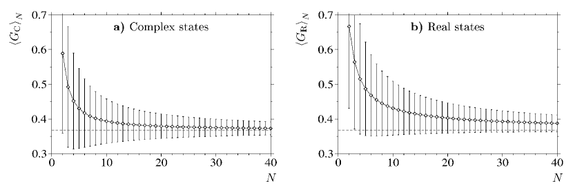
in FIG. 1 the mean values ${\langle G_{(\beta)}^{\phantom{2}}\rangle}_{N}^{\phantom{2}}$ and variance $\sigma^{2}_{N}={\langle G^{2}_{(\beta)}\rangle}_{N}^{\phantom{2}}-{\langle G_{(\beta)}^{\phantom{2}}\rangle}_{N}^{2}$ are represented as a function of $N$ for both complex and real cases.

Figure 1: Average of $G$–concurrence for (a) complex and (b) real random mixed states of a $N\times\left(N+2-\beta\right)$ system distributed according to the HS measure. The average is computed by means of equation (8); error bars represent the variance of $P_{N}^{(\beta)}(G)$. Dashed line represent the asymptote $G_{\star}=1/\textrm{e}$, whose explanation is given in Section V.

IV Probability distribution $P_{N}^{(\beta)}(G)$

This Section is devoted to the study of probability distributions. We shall start with the simplest problem of determining the distribution of the determinant $D$ of a $2\times 2$ density matrix $\rho_{2}$ distributed according to the (HS)–measure. In this case an explicit solution is easily obtained by integrating the Dirac delta $\delta(D-\Lambda_{1}\Lambda_{2})$ over the distribution $P^{(\beta)}_{\text{{HS}}}(\Lambda_{1},\Lambda_{2})$ of (5), that is

$$P_{2}^{(\beta)}(D):=C_{2}^{(1,\beta)}\int_{-\infty}^{\infty}\mathrm{d}\Lambda_{1}\int_{-\infty}^{\infty}\mathrm{d}\Lambda_{2}\,\delta(\Lambda_{1}+\Lambda_{2}-1)\,\theta(\Lambda_{1})\,\theta(\Lambda_{2})\,|\Lambda_{1}-\Lambda_{2}|^{\beta}\,\delta(D-\Lambda_{1}\Lambda_{2})\ \cdot$$

It is a very simple distribution since $(\Lambda_{1}-\Lambda_{2})^{2}=(\Lambda_{1}+\Lambda_{2})^{2}-4D=1-4D$. Thus

$$\begin{cases}P_{2}^{\mathds{C}}(D)&=6\>\sqrt{1-4D}\\ P_{2}^{\mathds{R}}(D)&=4\end{cases}\qquad,\qquad D\in\left[0,\frac{1}{4}\right]\ \cdot$$ (9)

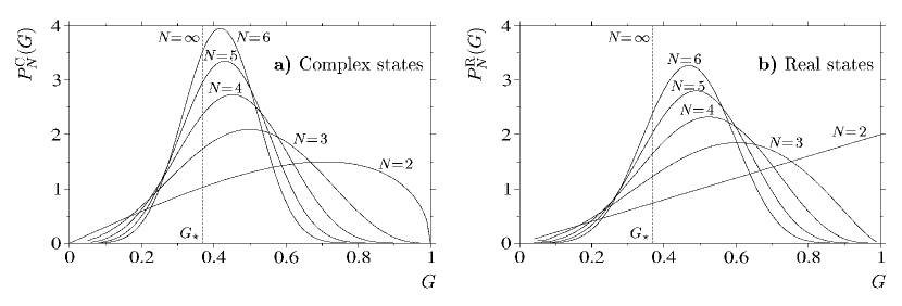
The $G$–concurrence distribution $P_{2}^{(\beta)}(G)$ can be computed either by integrating $\delta(G-2\sqrt{\Lambda_{1}\Lambda_{2}})$ over $P^{(\beta)}_{\text{{HS}}}(\Lambda_{1},\Lambda_{2})$, or simply using the latter result (9) together with $P_{2}^{(\beta)}(G)\>\mathrm{d}G=P_{2}^{(\beta)}(D)\>\mathrm{d}D$; in both cases (see FIG. 2)

$$\begin{cases}P_{2}^{\mathds{C}}(G)&=3\>G\>\sqrt{1-G^{2}}\\ P_{2}^{\mathds{R}}(G)&=2\>G\end{cases}\qquad,\qquad G\in\left[0,1\right]\ \cdot$$ (10)

Note that, due to $\Lambda_{1}+\Lambda_{2}=1$, (only) for the case $N=2$ the $G$–concurrence given by (1) reduces to the standard concurrence Wo98 , $C=\sqrt{2\left(1-\operatorname*{Tr}\rho_{2}^{2}\right)}$. Thus formula (10) for the complex case coincides with the distribution of concurrence $P(C)$ obtained in ZS01 .

For higher $N$ we will construct the distribution $P_{N}^{(\beta)}(D)$ from all moments $\langle D_{(\beta)}^{M}\rangle_{N}$ given by equation (7); indeed

$$\langle D^{M}_{(\beta)}\rangle_{N}=\int_{0}^{1}\mathrm{d}D\ D^{M}\ P_{N}^{(\beta)}(D)=\int_{0}^{\infty}\mathrm{d}x\ \textrm{e}^{-x(1+M)}P_{N}^{(\beta)}(\textrm{e}^{-x})\ ,$$

with $D={\rm e}^{-x}$ and $\mathrm{d}D=-\mathrm{d}x\ {\rm e}^{-x}$, and so we can obtain $P_{N}(D)$ by inverse Laplace transform or inverse Mellin transform as integral along the imaginary $M$–axis:

$$P_{N}^{(\beta)}(D)=\int_{-i\infty}^{+i\infty}\frac{\mathrm{d}M}{2\pi i}\ D^{-(1+M)}\ \langle D_{(\beta)}^{M}\rangle_{N}$$ (11)

Although equations (11) and (7) allow us to compute the $P_{N}^{(\beta)}(D)$ probabilities, the cognate quantities $P_{N}^{(\beta)}(G)$ can be determined as well by using

$$P_{N}^{(\beta)}(G)\>\mathrm{d}G=P_{N}^{(\beta)}(D)\>\mathrm{d}D\ ;$$

by taking from (1) the explicit expression for $\mathrm{d}D/\mathrm{d}G$, one can indeed get the simple expression

$$G\cdot P_{N}^{(\beta)}(G)=N\cdot D\cdot P_{N}^{(\beta)}(D)\ \cdot$$ (12)

From now on formulae and figures will be given indifferently for both $G$ and $D$ distribution, being clear their mutual relation. In particular the $D$–distribution is more indicated in showing details of calculation, for its simpler form, whereas the $G$–distribution better shows features in the pictures, for its domain being independent of $N$.

Figure 2: $G$–concurrence’s distributions $P_{N}^{(\beta)}(G)$ are compared for different $N$ in the case of (a) complex and (b) real random pure states. The distributions are obtained by performing numerically DALM the inverse Laplace transform of equation (11). Dashed vertical line centered in $G_{\star}=1/\textrm{e}$ denotes the position of the Dirac–delta corresponding to $P_{N\to\infty}^{(\beta)}(G)$, as it is shown in section V.

Important is the asymptotic behavior of the Gamma function for large argument (Stirling’s formula)

$$\Gamma(z)=z^{(z-1/2)}\sqrt{2\pi}\>\textrm{e}^{-z}\left[1+\frac{1}{12z}+{\mathcal{O}}{\left(\frac{1}{z}\right)}^{2}\right]$$

for $|z|\to\infty$ and $\arg(z)<\pi$. This implies the asymptotic behavior of (7) for large $|M|$:

$$\begin{cases}\rule[-12.91663pt]{0.0pt}{21.52771pt}\langle D^{M}_{\mathds{C}}\rangle_{N}&\simeq D^{\text{{S}}}_{\mathds{C}}\left(M,N\right):=A_{N}^{\mathds{C}}\cdot\frac{\textrm{e}^{-MN\log N}}{M^{(N^{2}-1)/2}}\\ \rule[-8.61108pt]{0.0pt}{21.52771pt}\langle D^{M}_{\mathds{R}}\rangle_{N}&\simeq D^{\text{{S}}}_{\mathds{R}}\left(M,N\right):=A_{N}^{\mathds{R}}\cdot\frac{\textrm{e}^{-MN\log N}}{M^{(N^{2}+N-2)/4}}\end{cases}\quad,\quad\text{with}\quad\begin{cases}\rule[-12.91663pt]{0.0pt}{21.52771pt}A_{N}^{\mathds{C}}:=\frac{(2\pi)^{(N-1)/2}\Gamma(N^{2})}{N^{N^{2}-1/2}\prod_{j=1}^{N}\Gamma(j)}\\ \rule[-8.61108pt]{0.0pt}{21.52771pt}A_{N}^{\mathds{R}}:=\frac{(2\pi)^{(N-1)/2}\Gamma\left[\left(N^{2}+N\right)/{2}\right]}{N^{(N^{2}+N-1)/2}\prod_{j=1}^{N}\Gamma\left[\left(j+1\right)/{2}\right]}\end{cases}\quad\cdot$$ (13)

As a consequence the integral (11) converges and moreover it vanishes if $x<N\log N$ or $D>(1/N)^{N}$, because in that case we can close the contour in (11) in the right $M$–halfplane according to the Jordan’s Lemma Ar85 . Physically this means that there are no density matrices with determinants greater than the one with maximal entropy.

In the rest of this section we will give the asymptotic behavior of distributions $P_{N}^{(\beta)}(D)$ for the two edges of the domain, that is $D\to 0$ and $D\to(1/N)^{N}$. The details of calculation, together with the explicit $N$–dependence of all coefficients listed here in the following, are collected in Appendix A.

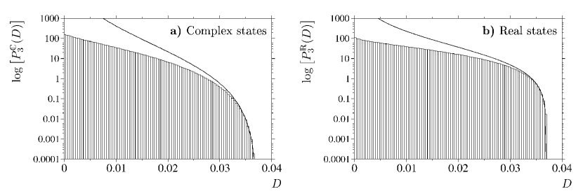
In particular, when very close to the completely mixed state, that is $D\simeq(1/N)^{N}$, we have the result (see FIG. 3)

$$\begin{cases}\rule[-12.91663pt]{0.0pt}{21.52771pt}P_{N}^{\mathds{C}}(D)\simeq A_{N}^{\mathds{C}}\cdot\frac{(-\log D-N\log N)^{(N^{2}-3)/2}}{D\ {\big{[}\left(N^{2}-3\right)/{2}\big{]}}{\displaystyle!}}\\ \rule[-8.61108pt]{0.0pt}{21.52771pt}P_{N}^{\mathds{R}}(D)\simeq A_{N}^{\mathds{R}}\cdot\frac{(-\log D-N\log N)^{(N^{2}+N-6)/4}}{D\ {\big{[}\left(N^{2}+N-6\right)/{4}\big{]}}{\displaystyle!}}\end{cases}\ \cdot$$ (14)

Figure 3: In panel (a) a $100$ bins histogram of $10^{8}$ determinants of $3\times 3$ complex density matrices distributed accordingly to the HS measure is compared with the right asymptote given by equation (14) (plotted in solid line). Same analysis is depicted in panel (b), but for $3\times 3$ real density matrices.

Moreover, using (12) together with

$$-\log D-N\log N\simeq 1-D\;N^{N}=1-G^{N}\quad,$$

we simply find

$$\begin{cases}\rule[-12.91663pt]{0.0pt}{21.52771pt}P_{N}^{\mathds{C}}(G)\simeq{\widetilde{A}}_{N}^{\mathds{C}}\cdot\frac{(1-G^{N})^{(N^{2}-3)/2}}{G}\\ \rule[-8.61108pt]{0.0pt}{21.52771pt}P_{N}^{\mathds{R}}(G)\simeq{\widetilde{A}}_{N}^{\mathds{R}}\cdot\frac{(1-G^{N})^{(N^{2}+N-6)/4}}{G}\end{cases}\quad,\quad\text{with}\quad\begin{cases}\rule[-12.91663pt]{0.0pt}{21.52771pt}{\widetilde{A}}_{N}^{\mathds{C}}:=A_{N}^{\mathds{C}}\cdot\frac{N}{\Gamma{\big{[}\left(N^{2}-1\right)/{2}\big{]}}}\\ \rule[-8.61108pt]{0.0pt}{21.52771pt}{\widetilde{A}}_{N}^{\mathds{R}}:=A_{N}^{\mathds{R}}\cdot\frac{N}{\Gamma{\big{[}\left(N^{2}+N-2\right)/{4}\big{]}}}\end{cases}\quad\cdot$$

For the other part of the spectrum, that is for very small $D$, the probability $P_{N}^{\mathds{C}}(D)$ can be expanded in a power series with some logarithmic corrections, as follows:

$$P_{N}^{\mathds{C}}(D)\simeq Z_{N}^{\mathds{C}}+X_{N}^{\mathds{C}}\cdot D\log D+{\widetilde{X}}_{N}^{\mathds{C}}\cdot D+V_{N}^{\mathds{C}}\cdot D^{2}\left(\log D\right)^{2}+{\widetilde{V}}_{N}^{\mathds{C}}\cdot D^{2}\left(\log D\right)+\widetilde{\widetilde{V}}{}_{N}^{\mathds{C}}\cdot D^{2}+{\cal O}\left(D^{3}(\log D)^{3}\right)$$ (15)

In particular, coefficients $Z_{N}^{\mathds{C}},X_{N}^{\mathds{C}},{\widetilde{X}}_{N}^{\mathds{C}}$ are computed in appendix A for all $N\geqslant 3$, whereas for $V_{N}^{\mathds{C}},{\widetilde{V}}_{N}^{\mathds{C}}$ and $\widetilde{\widetilde{V}}{}_{N}^{\mathds{C}}$ we limit ourself to explicitly solve the case $N=3$ (the case $N=2$ is simply given by formula (9)).

Figure 4: In panel (a), formula (10) is compared with a $100$ bins histogram of $10^{6}$ $G$–concurrence of $2\times 2$ complex density matrices distributed according to the HS measure. The other panels (b) (c) and (d) shows histograms (for different $N$) together with the distribution of $G$–concurrence obtained by inverse Laplace transforming as in equation (11) (plotted in solid lines). The left asymptote given by eq. (15), computed up to ${\cal O}\left(D\right)$, is also plotted in dashed line for comparison; in panel (b) we also add the contribution given by $V_{N}^{\mathds{C}},{\widetilde{V}}_{N}^{\mathds{C}},\widetilde{\widetilde{V}}{}_{N}^{\mathds{C}}$ coefficients, using a dotted line.

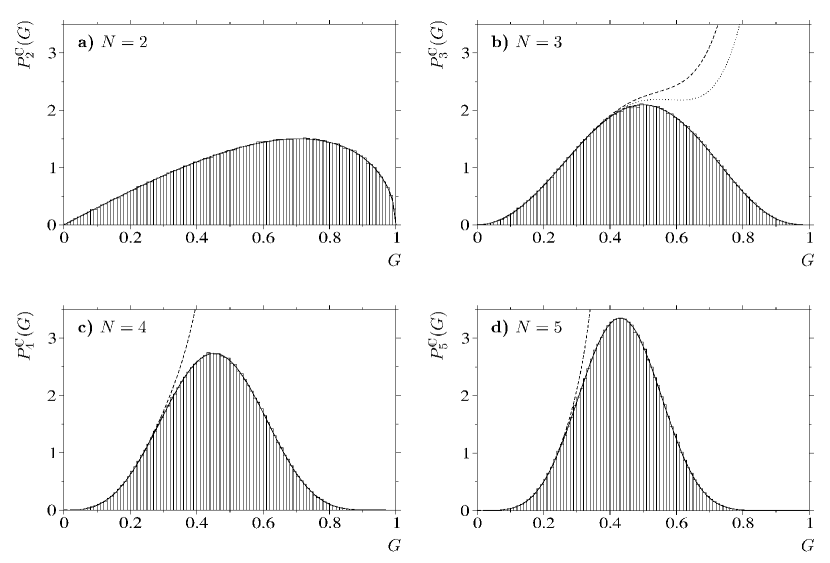
The situation is similar when we do consider, in the same region of the domain, the probability $P_{N}^{\mathds{R}}(D)$, corresponding to small determinants of reduced $N\times N$ real density matrices HS–distributed. The expansion is still a power series (plus logarithmic corrections) but the exponents are now semi–integer, according to the mechanism described in Appendix A, thus the probability reads:

$$P_{N}^{\mathds{R}}(D)\simeq Z_{N}^{\mathds{R}}+Y_{N}^{\mathds{R}}\cdot D^{\frac{1}{2}}+X_{N}^{\mathds{R}}\cdot D\log D+{\widetilde{X}}_{N}^{\mathds{R}}\cdot D+W_{N}^{\mathds{R}}\cdot D^{\frac{3}{2}}\log D+{\widetilde{W}}_{N}^{\mathds{R}}\cdot D^{\frac{3}{2}}+{\cal O}\left(D^{2}(\log D)^{2}\right)$$

V Concentration of $G$–concurrence for large system size

Iterating the recursion relation for the Gamma function $\Gamma\left(n+1\right)=n\>\Gamma\left(n\right)$, we can recast expression (8) of the $M$– moment of the $G$–concurrence of complex random pure state as

$$\left<G_{\mathds{C}}^{M}\right>_{N}=\left\{\prod_{k=0}^{M-1}\frac{N}{N^{2}+k}\right\}\left\{\left[\frac{M}{N}\;\Gamma\left(\frac{M}{N}\right)\right]^{N}\right\}\left\{\prod_{k=1}^{N-1}\left(1+\frac{M}{kN}\right)^{N-k}\right\}\quad,$$

with the asymptotics characterized with help of the Euler constant $\gamma\approx 0.\,577\;215\;665\ldots$,

$$\prod_{k=0}^{M-1}\frac{N}{N^{2}+k} \xrightarrow[\ N\to\infty\ ]{}\frac{1}{N^{M}}\quad,$$

$$\left[\frac{M}{N}\;\Gamma\left(\frac{M}{N}\right)\right]^{N} \xrightarrow[\ N\to\infty\ ]{}\textrm{e}^{-\gamma M}$$

and

$$\prod_{k=1}^{N-1}\left(1+\frac{M}{kN}\right)^{N-k} \xrightarrow[\ N\to\infty\ ]{}N^{M}\textrm{e}^{M(\gamma-1)}\quad,$$

so that finally

$$\left<G_{\mathds{C}}^{M}\right>_{N} \xrightarrow[\ N\to\infty\ ]{}\textrm{e}^{-M}\quad\cdot$$ (16)

For the analogue moments of $G$–concurrence of real random pure state, some technicality requires that the sequence of odd and even $N$ has to be analyzed separately, although it is not hard to prove that the limit is the same. For that reason, we will simply illustrate the case $N=2p$, $p\in\mathds{N}$, for which (8) gives

$$\left<G_{\mathds{R}}^{M}\right>_{N}={\left(\frac{2}{\sqrt{\pi}}\right)}^{p}\left\{\prod_{k=0}^{M-1}\frac{2p}{2p^{2}+p+k}\right\}\left\{\left[\frac{M}{2p}\;\Gamma\left(\frac{M}{2p}\right)\right]^{p}\right\}\left\{\left[\left(\frac{M}{2p}+\frac{1}{2}\right)\;\Gamma\left(\frac{M}{2p}+\frac{1}{2}\right)\right]^{p}\right\}\times\\ \times\left\{\prod_{k=1}^{p-1}\left(1+\frac{M}{2pk}\right)^{p-k}\right\}\left\{\prod_{k=\frac{3}{2}}^{p-\frac{1}{2}}\left(1+\frac{M}{2pk}\right)^{p-k-\frac{1}{2}}\right\}\quad,$$ (17)

with

$$\prod_{k=0}^{M-1}\frac{2p}{2p^{2}+p+k} \xrightarrow[\ p\to\infty\ ]{}{\left(\frac{2}{2p+1}\right)}^{M}\quad,$$

$$\left[\frac{M}{2p}\;\Gamma\left(\frac{M}{2p}\right)\right]^{p} \xrightarrow[\ p\to\infty\ ]{}\textrm{e}^{-\gamma\frac{M}{2}}\quad,$$

$$\left[\left(\frac{M}{2p}+\frac{1}{2}\right)\;\Gamma\left(\frac{M}{2p}+\frac{1}{2}\right)\right]^{p} \xrightarrow[\ p\to\infty\ ]{}\frac{\pi^{\frac{p}{2}}}{2^{\left(p+M\right)}}\>\textrm{e}^{M\left(1-\frac{\gamma}{2}\right)}\quad,$$

$$\prod_{k=1}^{p-1}\left(1+\frac{M}{2pk}\right)^{p-k} \xrightarrow[\ p\to\infty\ ]{}p^{\frac{M}{2}}\textrm{e}^{\frac{M}{2}\left(\gamma-1\right)}$$

and

$$\prod_{k=\frac{3}{2}}^{p-\frac{1}{2}}\left(1+\frac{M}{2pk}\right)^{p-k-\frac{1}{2}} \xrightarrow[\ p\to\infty\ ]{}\textrm{e}^{\frac{M}{2}\left(\gamma-1\right)}\textrm{e}^{-M}\>2^{M}{\left(p+\frac{1}{2}\right)}^{\frac{M}{2}}\quad\cdot$$

Putting all factors together we arrive at the general result (compare with (16))

$$G(M):=\lim_{N\to\infty}\left<G_{\left(\beta\right)}^{M}\right>_{N}=\textrm{e}^{-M}\qquad\cdot$$ (18)

The above expression, valid for both $\beta\in\left\{1,2\right\}$, is useful to derive the limiting distribution

$$P^{\left(\beta\right)}(G):=\lim_{N\to\infty}P_{N}^{\left(\beta\right)}(G)\quad\cdot$$

We see from (18) that its average is $1/\textrm{e}=0.\,367\>879\>441\ldots$ and its variance is $0$; such behavior can be recognized in FIG 1. Moreover, by fixing $G=\textrm{e}^{-x}$, one can see that $G(M)$ of (18) is nothing but the Laplace transform of the function

$$\eta(x):=\textrm{e}^{-x}P^{\left(\beta\right)}(\textrm{e}^{-x})$$

so that, by inverse Laplace transforming, we obtain

$$\textrm{e}^{-x}P^{\left(\beta\right)}(\textrm{e}^{-x})=G\>P^{\left(\beta\right)}(G)=\delta(-\log(G)-1)\quad\cdot$$

Rewriting the argument of the Dirac delta we finally arrive at

$$P^{\left(\beta\right)}(G)=\delta(G-\textrm{e}^{-1})\ \cdot$$ (19)

In other words, we have shown that for large systems the G–concurrence of random states is localized arbitrarily close to the averaged value.

A similar concentration effect has recently been quantified Ha06 for bipartite $N\times K$ systems. In particular the Von Neumann entropy of the reduced density matrix of the first subsystem concentrates around the entropy of the maximally mixed state, $S\left(\mathds{1}/N\right)=\log N$, if we let the dimension $K$ of the auxiliary subsystem to go to infinity faster than $N$. When $K=N$, so that the induced distribution coincides with the Hilbert–Schmidt distribution, and $N\to\infty$, then von Neumann entropy concentrate around $\log N-1/2$ SZ04 ; Ha06 . Remarkably, $G$–concurrence displays a similar concentration effect; moreover, we are in position to prove the convergence of its distribution to a Dirac delta centered at a non trivial value $1/\text{e}$.

The determinants and $G$–concurrence may be also averaged in the general case of asymmetric induced measure (2). Consider an interesting case $K>N$. As for the HS–distribution discussed in Section II the expectation value and the higher moments may be expressed as a ratio of normalization constants (2b) and (5b). For instance, the moments read

$${\rule[-6.45831pt]{0.0pt}{19.37494pt}\ \begin{cases}\displaystyle\rule[-23.68048pt]{0.0pt}{10.76385pt}\langle G^{M}_{\mathds{C}}\rangle_{N,K}&=N^{M}\frac{B^{(2)}_{N,K}}{C_{N}^{(M/N+K-N+1\>,\>2)}}=\ \displaystyle N^{M}\ \frac{\Gamma\left(NK\right)}{\Gamma\left(NK+M\right)}\ \prod_{j=1}^{N}\ \frac{\Gamma\left(K\,-\,N\,+\,j\;+\;{M}/{N}\right)}{\Gamma\left(K\,-\,N\,+\,j\right)}\\ \langle G^{M}_{\mathds{R}}\rangle_{N,K}\displaystyle&=N^{M}\frac{B^{(1)}_{N,K}}{C_{N}^{(M/N+(K-N+1)/2\>,\>1)}}=\ \displaystyle N^{M}\ \frac{\Gamma\left({NK}/{2}\right)}{\Gamma\left({NK}/{2}+M\right)}\ \prod_{j=1}^{N}\ \frac{\Gamma\left[\left(K\,-\,N\,+\,j\right)/{2}+{M}/{N}\right]}{\Gamma\left[\left(K\,-\,N\,+\,j\right)/{2}\right]}\end{cases}\quad\cdot\ }$$ (20)

Let us now study a particular case of the induced measure, for which we consider bipartite systems of arbitrarily large dimension, with the only constraint that the ratio between the size $K$ of the ancilla and the size $N$ of the principal subsystem are fixed and greater than one. Let this ratio be expressed by the rational number $q=\ell_{2}/\ell_{1}$, with the $\ell_{1}$ and $\ell_{2}$ integers; this means that we are considering systems with $N=J\ell_{1}<K=J\ell_{2}$.

With the same tools used in computing (18), one can let $J$ go to infinity and obtain

$$\rule[-6.45831pt]{0.0pt}{19.37494pt}\ G(M) \coloneqq\lim_{J\to\infty}\left<G_{\left(\beta\right)}^{M}\right>_{J\ell_{1},J\ell_{2}}=X_{q}^{-M}\quad,\quad\forall\ \beta\in\left\{1,2\right\}\quad,$$ (21)

with

$$X_{q} \coloneqq\;\frac{1}{\textrm{e}}\ {\left(\frac{q}{q-1}\right)}^{q-1}\quad,\quad q>1\quad\cdot$$ (22)

The limiting distribution $P_{q}(G)$, can be earned as before and reads

$$\rule[-6.45831pt]{0.0pt}{19.37494pt}\ P^{(\beta)}_{q}(G)\coloneqq\lim_{J\to\infty}P_{J\ell_{1},J\ell_{2}}^{(\beta)}(G)=\delta(G-X_{q})\quad,\,\$$

for the complex as well as for the real case. Although the accumulation point $X_{q}$ is not defined for the case $q=1$ (that is the case in which states in the principal system are HS–distributed), we find however $\lim_{q\rightarrow 1}X_{q}=1/\textrm{e}$, confirming our previous result (19). Moreover such values represent an infimum for $X_{q}$, whereas it attains the supremum on the other part of the domain, that is for $q\rightarrow\infty$. Such case correspond an extremely large environment, for which $X_{\infty}=1$, that is in turn the $G$–concurrence of the completely mixed state. Thus we find another evidence that large environment concentrates reduced density matrices around the maximally mixed states Ha06 .

VI Concluding remarks

The generalized $G$–concurrence is likely to be the first measure of pure state entanglement for which one could find not only the mean value over the set of random pure states, but also compute explicitly all moments and describe its probability distribution, deriving an analytic expression in the large $N$ limit. This offers for our work various potential applications. On one hand, analyzing a concrete quantum state and its entanglement we may check, to what extend its properties are non typical. In practice this can be done by a comparison of its $G$–concurrence $G$ with the mean value $\langle G\rangle$, and by comparing its deviation from the average, $|G-\langle G\rangle|$, with the root of the variance of the distribution.

On the other hand, if one needs a quantum state of some particular properties, one may estimate how difficult it is to obtain such a state at random. For instance, looking for a state of a large degree of entanglement, with concurrence greater than a given value $\widetilde{G}$, one can make use of the derived probability distribution by integrating it from $\widetilde{G}$ to unity in order to evaluate the probability to generate the desired state by a fully uncontrolled, chaotic quantum evolution.

Although in this work we have concentrated our attention on pure states of bipartite systems, the averages obtained for the asymmetric induced measures (2) with $K>N$ may be easily applied for the more general, multipartite case. Consider a system containing $n$ qudits (particles described in a $d$–dimensional Hilbert space). This system may be divided by an arbitrary bi–partite splitting into $m$ and $(n-m)$ particles, and one can study entanglement between both subsystems – see e.g. KZM02 . The partial trace over $m$ qudits is equivalent to the partial trace performed over a single ancilla of size $K=d^{m}$, so setting size of the system $N=d^{n-m}$ one may read out the average concurrence from eq. (20). In particular, if $n$ is even and we put $m=n/2+k$, then the ratio $q=K/N$ is equal to $d^{2k}$ and in the asymptotic limit $n\to\infty$ the concurrence concentrates around the mean (22) which depends only on the asymmetry $k$ of the splitting.

Our research may also be considered as a contribution to the random matrix theory: we have found the distribution of the determinants of random Wishart matrices $AA^{\dagger}$, normalized by fixing their trace. Furthermore, the analysis of the distribution of $G$-concurrence in the limit of large system sizes provides an illustrative example of the geometric concentration effect, since in high dimensions the distribution of the determinant is well localized around the mean value. This observation can also be related to the central limit theorem applied to logarithms of the eigenvalues of a density matrix, the sum of which is equal to the logarithm of the determinant.

It is a pleasure to thank P. Hayden and P. Horodecki for stimulating discussions. This work was financed by the SFB/Transregio–12 project financed by DFG. We also acknowledge support provided by the EU research project COCOS and the grant $1$  P$03$B  $042$  $26$ of Polish Ministry of Science and Information Technology.

Appendix A Coefficients of asymptotic expansions of probability

A.1 Right asymptote of $P_{N}^{(\beta)}(D)$: proof of equation (14)

The starting point is integral (11). Since all the poles of the integrand are in the left half–plane (see it in (7)), the contour integration along the imaginary axis can be modified into the one along the right asymptotic half–plane, that is on a very large semicircle connecting $-i\infty$ to $+i\infty$; this allow us to use the Stirling’s formula for replacing $\langle D^{M}_{\left(\beta\right)}\rangle_{N}$ with $D^{\text{{S}}}_{\left(\beta\right)}\left(M,N\right)$ (see formula (13)) in the integrand of (11). Of course we made an approximation, but we know that the formula we ended up matches the correct result ($P_{N}^{(\beta)}(D)=0$ for $D>{\left(1/N\right)}^{N}$) in the point ${\left(1/N\right)}^{N}$, so that such approximation would hold close to that point. Now we observe that $D^{\text{{S}}}_{\left(\beta\right)}\left(M,N\right)$ has poles only in $M=0$, so that our contour of integration can be modified provided that we do not cross the origin, and we do so obtaining

$$P_{N}^{(\beta)}(D)=\int_{\gamma}\frac{\mathrm{d}M}{2\pi i}\ D^{-(1+M)}\ D^{\text{{S}}}_{\left(\beta\right)}\left(M,N\right)=\frac{A_{N}^{\left(\beta\right)}}{2\pi iD}\int_{\gamma}{\mathrm{d}M}\ {\textrm{e}^{M\left(-\log D-N\log N\right)}M^{-\frac{(N^{2}-1)}{2}}}\quad,$$

where $\gamma$ is now the contour that, starting from $-i\infty$ get close to the negative real axis on the asymptotic left–lower quarter–plane, winds around $\mathds{R}^{-}\cup\left\{0\right\}$ in the counterclockwise direction, and then approaches $+i\infty$ on the asymptotic left–upper quarter–plane. But now we apply once more Jordan’s Lemma and we remove the asymptotic semi–circle from $\gamma$. After rescaling $M\to-M/\varepsilon$, with the latter defined by $\varepsilon=-\log D-N\log N$ and close to $1$, we arrive at the well known Hankel’s contour integral for the inverse of the Gamma function ($1/\Gamma$) AS70 , that leads to (14) and gives the asymptotic behavior for $D\to(1/N)^{N}$.

A.2 Left asymptote of $P_{N}^{\mathds{C}}(D)$ for complex random pure states

Now let us consider the behavior of $P^{\mathds{C}}_{N}(D)$ at the lower edge of the spectrum $D\to 0$. In that case one can close the integral (11) in the left halfplane obtaining contributions from all the poles of the Gamma functions in $\langle D^{M}_{\mathds{R}}\rangle_{N}$ (see (7)). Such poles are located at each of the negative integers $M=-1,-2,-3,\ldots$; fortunately there is the factor $D^{-(1+M)}$ such that we obtain a series in powers of $D$. Because of the multiple Gamma functions in (7), most of the poles are degenerate and the general feature (for an arbitrary large $N$) is that the pole in $-\ell$ is of order $\ell$: due to this fact the $D$–powers in the expansion get in general a logarithmic correction. The first pole at $M_{1}=-1$ is non degenerate and yields

$$P^{\mathds{C}}_{N}(0)=\frac{\Gamma(N^{2})}{\Gamma(N^{2}-N)\;\Gamma(N)}=Z_{N}^{\mathds{C}}\quad\cdot$$

Including the next order–2 pole ($M_{2}=-2$) contribution we find the asymptotic expansion for $D\to 0$

$$P_{N}^{\mathds{C}}(D)\simeq Z_{N}^{\mathds{C}}+X_{N}^{\mathds{C}}\cdot D\log D+{\widetilde{X}}_{N}^{\mathds{C}}\cdot D$$

with

$$\begin{cases}X_{N}^{\mathds{C}}&=\frac{\displaystyle\Gamma(N^{2})}{\displaystyle\Gamma(N^{2}-2N)\;\Gamma(N)\;\Gamma(N-1)}\rule[-12.91663pt]{0.0pt}{21.52771pt}\\ {\widetilde{X}}_{N}^{\mathds{C}}&={\textstyle X_{N}^{\mathds{C}}\Big{(}N+N\psi(N^{2}-2N)-4-2\psi(1)-(N-2)\psi(N-2)\Big{)}}\end{cases}\quad\cdot$$ (23)

Here $\psi(x)$ is the Digamma function , or polygamma function of order $0$, with

$$\psi(1)=-\gamma,\qquad\psi(n)=-\gamma+\sum_{k=1}^{n-1}\frac{1}{k},\text{\ for\ }n>1\ .\$$ (24)

Note that the Euler constant $\gamma$ cancels everywhere. By adding the next order–3 pole ($M_{3}=-3$) contribution one gets in general the terms in (15) corresponding to the $V_{N}^{\mathds{C}},{\widetilde{V}}_{N}^{\mathds{C}}$ and $\widetilde{\widetilde{V}}{}_{N}^{\mathds{C}}$ coefficients, although the latter are in general rather complicated, involving polygamma function of order higher than $0$. This is not the case when $N=3$, for which a cancelation makes $M_{3}=-3$ a pole of order $2$, and the coefficients read :

$$V_{3}^{\mathds{C}}=0\qquad,\qquad{\widetilde{V}}_{3}^{\mathds{C}}=6\cdot 7!=30\,240\qquad,\qquad\widetilde{\widetilde{V}}{}_{3}^{\mathds{C}}=9\cdot 7!=45\,360\qquad\cdot\$$

A.3 Left asymptote of $P_{N}^{\mathds{R}}(D)$ for real random pure states

We will apply the same reasoning of the previous case, just now differing for the fact that, when $\beta=1$, the $\ell^{\text{th}}$ pole $M_{\ell}$ of the integrand of (11) is $-\frac{\ell+1}{2}$; in general, for arbitrarily large $N$, its corresponding order is given by $\left\lfloor\frac{\ell+1}{2}\right\rfloor$, where $\left\lfloor x\right\rfloor$ means the larger integer not exceeding $x$. In particular, the firsts two poles $M_{1}=-1$ and $M_{2}=-\frac{3}{2}$ are non degenerate and yield 

$$Z_{N}^{\mathds{R}}=\frac{2^{N-1}\;\Gamma\big{(}\frac{N^{2}+N}{2}\big{)}}{\Gamma\left(\frac{N^{2}-N}{2}\right)\;\Gamma\left(N\right)}\qquad\text{and}\qquad Y_{N}^{\mathds{R}}=-\sqrt{\pi}\frac{2^{N-1}\;\Gamma\big{(}\frac{N^{2}+N}{2}\big{)}}{\Gamma\left(\frac{N^{2}-2N}{2}\right)\;\Gamma\left(\frac{N+1}{2}\right)\;\Gamma\left(N-1\right)}\qquad\cdot$$

Including the next two $2$–order poles contributions ($M_{3}=-2$ and $M_{4}=-\frac{5}{2}$) we determine, for $N>3$

$$\begin{cases}X_{N}^{\mathds{R}}&=-\frac{2^{2N-3}\;\Gamma\big{(}\frac{N^{2}+N}{2}\big{)}}{\Gamma\left(\frac{N^{2}-3N}{2}\right)\;\Gamma\left(N\right)\;\Gamma\left(N-2\right)}\rule[-12.91663pt]{0.0pt}{21.52771pt}\\ {\widetilde{X}}_{N}^{\mathds{R}}&={\textstyle X_{N}^{\mathds{R}}\left\{N+N\psi\left(\frac{N^{2}-3N}{2}\right)-8-\frac{3}{2}\>\psi\left(\frac{1}{2}\right)-2\>\psi\left(1\right)-\frac{N-3}{2}\>\psi\left(\frac{N-3}{2}\right)-\frac{N-4}{2}\>\psi\left(\frac{N-4}{2}\right)\right\}}\end{cases}\quad,$$ (25)

and for $$N>4$$

$$\begin{cases}W_{N}^{\mathds{R}}&=-\frac{\sqrt{\pi}}{3}\frac{2^{2N-3}\;\Gamma\big{(}\frac{N^{2}+N}{2}\big{)}}{\Gamma\left(\frac{N^{2}-4N}{2}\right)\;\Gamma\left(\frac{N+1}{2}\right)\;\Gamma\left(N-1\right)\;\Gamma\left(N-3\right)}\rule[-12.91663pt]{0.0pt}{21.52771pt}\\ {\widetilde{W}}_{N}^{\mathds{R}}&={\textstyle W_{N}^{\mathds{R}}\left\{N+N\psi\left(\frac{N^{2}-4N}{2}\right)-\frac{35}{3}-\frac{5}{2}\>\psi\left(\frac{1}{2}\right)-2\>\psi\left(1\right)-\frac{N-4}{2}\>\psi\left(\frac{N-4}{2}\right)-\frac{N-5}{2}\>\psi\left(\frac{N-5}{2}\right)\right\}}\end{cases}\quad,$$ (26)

where we made use once more of the $\psi$–digamma function  of (24). The case $N=3$ constitutes an exception for $X_{3}^{\mathds{R}}$ and $W_{3}^{\mathds{R}}$’s coefficients, because of the lowering of the order of $M_{3}$ and $M_{4}$ poles; moreover, for the latter pole, the same happens also for $N=4$. All these coefficients need separate calculations and read

$${\widetilde{X}}_{3}^{\mathds{R}}=12\cdot 5!\hskip 8.61108pt,\hskip 8.61108pt{\widetilde{W}}_{3}^{\mathds{R}}=4\cdot 5!\hskip 8.61108pt,\hskip 8.61108pt{\widetilde{W}}_{4}^{\mathds{R}}=2^{8}\cdot 8!\hskip 17.22217pt\text{and}\hskip 17.22217ptX_{3}^{\mathds{R}}=W_{3}^{\mathds{R}}=W_{4}^{\mathds{R}}=0\hskip 8.61108pt\cdot$$

References

- (1) M. A. Nielsen and I. L. Chuang, Quantum Computation and Quantum Information, Cambridge University Press, Cambridge, 2000.
- (2) F. Haake Quantum Signatures of Chaos, Springer, Berlin, 1990.
- (3) V. Vedral and M. B. Plenio, Phys. Rev. A 57, 1619 (1998).
- (4) M. Horodecki, Quant. Inf. Comp. 1, 3 (2001).
- (5) M. B. Plenio and S. Virmani preprint quant-ph/0504163
- (6) I. Bengtsson and K. Życzkowski, Geometry of quantum states: An introduction to quantum entanglement, Cambridge University Press, Cambridge 2006.
- (7) A. Peres, Quantum Theory: Concepts and Methods, Kluver, Dordrecht 1993.
- (8) G. Vidal, J. Mod. Opt. 47, 355 (2000).
- (9) M. Sinołȩcka, K. Życzkowski and M. Kuś, Acta Phys. Pol. B 33, 2081–2095 (2002).
- (10) G. Gour, Phys. Rev. A 71, 012318 (2005).
- (11) K. Horodecki, M. Horodecki and P. Horodecki preprint quant-ph/0512224
- (12) G. Gour, Phys. Rev. A 72, 042318 (2005).
- (13) K. Życzkowski and H.–J. Sommers, J. Phys. A 34, 7111–7125 (2001).
- (14) S. Lloyd and H. Pagels, Ann. Phys. (N.Y.), 188, 186 (1988).
- (15) M. L. Mehta Random Matrices II ed. (New York: Academic) 1991.
- (16) K. Życzkowski and H.–J. Sommers, J. Phys. A 36, 10115–10130 (2003).
- (17) W. K. Wootters, Phys. Rev. Lett. 80, 2245 (1998).
- (18) L. D’Amore, G. Laccetti and A. Murli, ACM Transactions on Mathematical Software (TOMS), 25(3), 306–315 (1999).
- (19) G. Arfken, Mathematical Methods for Physicists, 3rd ed., FL: Academic Press, Orlando 1985.
- (20) P. M. Hayden, D. W. Leung and A. Winter, Comm. Math. Phys. 265(1), 95 (2006)
- (21) H.–J. Sommers and K. Życzkowski, J. Phys. A 37, 8457 (2004).
- (22) V.M. Kendon, K. Życzkowski, and W.J. Munro Phy. Rev. A 66 062310 (2002)
- (23) M. Abramowitz and I. A. Stegun, Handbook of Mathematical Functions, Washington, D.C. 1970.