Quantum Entanglement and Projective Ring Geometry

Quantum Entanglement
and Projective Ring Geometry

Michel PLANAT ^†, Metod SANIGA ^‡ and Maurice R. KIBLER ^§ M. Planat, M. Saniga and M.R. Kibler

^† Institut FEMTO-ST, CNRS/Université de Franche-Comté, Département LPMO,
  32 Avenue de l’Observatoire, F-25044 Besançon Cedex, France planat@lpmo.edu

^‡ Astronomical Institute, Slovak Academy of Sciences,
  SK-05960 Tatranská Lomnica, Slovak Republic msaniga@astro.sk

^§ Institut de Physique Nucléaire de Lyon, IN2P3-CNRS/Université Claude Bernard Lyon 1,
  43 Boulevard du 11 Novembre 1918, F-69622 Villeurbanne Cedex, France kibler@ipnl.in2p3.fr

Received June 13, 2006, in final form August 16, 2006; Published online August 17, 2006

The paper explores the basic geometrical properties of the observables characterizing two-qubit systems by employing a novel projective ring geometric approach. After introducing the basic facts about quantum complementarity and maximal quantum entanglement in such systems, we demonstrate that the $15\times 15$ multiplication table of the associated four-dimensional matrices exhibits a so-far-unnoticed geometrical structure that can be regarded as three pencils of lines in the projective plane of order two. In one of the pencils, which we call the kernel, the observables on two lines share a base of Bell states. In the complement of the kernel, the eight vertices/observables are joined by twelve lines which form the edges of a cube. A substantial part of the paper is devoted to showing that the nature of this geometry has much to do with the structure of the projective lines defined over the rings that are the direct product of $n$ copies of the Galois field $GF(2)$, with $n=2,3$ and 4.

quantum entanglement; two spin-$\frac{1}{2}$ particles; finite rings; projective ring lines

81P15; 51C05; 13M05; 13A15; 51N15; 81R05

1 Introduction

“Seriousness” of quantum theory for addressing the most fundamental aspects of reality has invariably been at the forefront of theoretical explorations of most prominent scholars [1, 2, 3, 4, 5, 6], being firmly established by experiment in 1982 [7]. Two measurements described by non-commuting observables are inherently uncertain and this led Einstein, Podolsky and Rosen [1] to question the completeness of quantum theory versus the reality of both observed physical quantities. Using counterfactual arguments applied to distant experimental set-ups they introduced (and immediately rejected) the notion of underlying wholeness, which shortly after gave rise to the concept of quantum entanglement [8]. Bohr believed that no serious conclusion can be drawn from the comparison of thought experiments dealing with mutually incompatible (i.e., non-commuting) observables and thus practically ignored the paradox, proposing another view/paradigm–quantum complementarity [10]. Since the work of Bohm [2] and Bell [3], the “puzzles” of quantum theory have mainly been discussed within a discrete variable setting of spin-$\frac{1}{2}$ particles. In essence, Bell’s theorems [6] imply that either the recursive (counterfactual) reasoning about possible experiments should be abandoned, or non-contextual assumptions (implicit in the EPR locality arguments) are to be challenged, or both. One of the simplest illustrations of quantum “mysteries”, which also provides a very economical proof of the Bell–Kochen–Specker theorem [3, 4], employs a $3\times 3$ array of nine observables characterizing two spin-$\frac{1}{2}$ particles [6]. The three operators in any row or column of such a square, commonly referred to as the Mermin “magic” square, are mutually commuting, allowing the recursive reasoning to be used, but the algebraic structure of observables contradicts that of their eigenvalues [6]. This contradiction stems from the following two basic features of the structure of the square: complementarity between the observables located in two distinct rows and two of the columns and the maximal entanglement of the observables in one of the columns.

The basic facts about quantum complementarity and maximal quantum entanglement for two spin-$\frac{1}{2}$ particles (or two-qubits, using the language of quantum information theory) are given in Section 2. In Section 3 we demonstrate that the $15\times 15$ multiplication table of the associated four-dimensional (generalized Pauli spin) matrices exhibits a so-far-unnoticed geometrical structure, which can be regarded as three pencils of lines in the projective plane of order two (the Fano plane) [11]. These three pencil-configurations, each featuring seven points/observables, share a line (called the reference line), and any line comprises three observables, each being the product of the other two, up to a factor $-1$, $i$ or $-i$ ($i^{2}=-1$). All the three lines in each pencil carry mutually commuting operators; in one of the pencils, which we call the kernel, the observables on two lines share a base of maximally entangled states. The three operators on any line in each pencil represent a row or column of some of Mermin’s “magic” squares, thus revealing an inherent geometrical nature of the latter [12, 13]. In the complement of the kernel, the eight vertices/observables are joined by twelve lines which form the edges of a cube. The lines between the kernel and the cube are pairwise complementary, which means that each vertex/observable is linked with six other ones.

Some of these intriguing geometrical features can be recovered, as shown in detail in Section 4, in terms of the structure of the projective line defined over the finite ring $GF(2)^{\otimes n}$, with $n=2,3,4$, $GF(2)\cong\mathcal{Z}_{2}$ denoting the Galois field with two elements and $\otimes n$ representing the direct product of $n$ such fields. After recalling some basics on the concept of a projective ring line and the associated concepts of neighbour and distant, we illustrate its basic properties over the ring $GF(2)^{\otimes 2}$ and show that the corresponding line reproduces nicely all the basic qualitative properties of a Mermin square (Section 4.1). In order to account for a more intricate geometrical structure of the kernel and the cube, one has to employ the lines corresponding to $n=3$ (Section 4.2) and $n=4$ (Section 4.3), respectively. Although these two lines provide us with important insights into the structure of the two operator configurations, it is obvious we will have to look for a higher order ring line in order to get a more complete geometrical picture of two-qubit systems.

2 Quantum complementarity, maximal entanglement
and mutually unbiased bases

Table 1: Multiplication between the elements of $\mathcal{A}$.

$*$	$0$	$1$	$2$	$3$	$6$	$14$	$9$	$12$
0	$0$	$1$	$2$	$3$	$6$	$14$	$9$	$12$
1	$1$	$0$	$3$	$2$	$-i14$	$i6$	$-i12$	$i9$
2	$2$	$3$	$0$	$1$	$i9$	$i12$	$-i6$	$-i14$
3	$3$	$2$	$1$	$0$	$12$	$-9$	$-14$	$6$
6	$6$	$i14$	$-i9$	$12$	$0$	$-i1$	$i2$	$3$
14	$14$	$-i6$	$-i12$	$-9$	$i1$	$0$	$-3$	$-i2$
9	$9$	$i12$	$i6$	$-14$	$-i2$	$-3$	$0$	$-i1$
12	$12$	$-i9$	$i14$	$6$	$3$	$i2$	$i1$	$0$

Table 2: Multiplication between the elements of $\mathcal{B}$.

$*$	$4$	$7$	$11$	$13$	$5$	$10$	$15$	$8$
4	$0$	$1$	$i2$	$i3$	$6$	$14$	$-i9$	$-i12$
7	$1$	$0$	$i3$	$i2$	$-i14$	$i6$	$-12$	$9$
11	$-i2$	$-i3$	$0$	$1$	$9$	$12$	$i6$	$i14$
13	$-i3$	$-i2$	$1$	$0$	$-i12$	$i9$	$14$	$-6$
5	$6$	$i14$	$9$	$i12$	$0$	$-i1$	$2$	$-i3$
10	$14$	$-i6$	$12$	$-i9$	$i1$	$0$	$i3$	$2$
15	$i9$	$-12$	$-i6$	$14$	$2$	$-i3$	$0$	$-i1$
8	$i12$	$9$	$-i14$	$-6$	$i3$	$2$	$i1$	$0$

Table 3: Multiplication between the elements of $\mathcal{A}$ and $\mathcal{B}$.

$*$	$0$	$1$	$2$	$3$	$6$	$14$	$9$	$12$
4	$4$	$7$	$-i11$	$-i13$	$5$	$10$	$i15$	$i8$
7	$7$	$4$	$-i13$	$-i11$	$-i10$	$i5$	$8$	$-15$
11	$11$	$13$	$i4$	$i7$	$-i15$	$-i8$	$5$	$10$
13	$13$	$11$	$i7$	$i4$	$-8$	$15$	$-i10$	$i5$
5	$5$	$i10$	$15$	$i8$	$4$	$-i7$	$11$	$-i13$
10	$10$	$-i5$	$8$	$-i15$	$i7$	$4$	$i13$	$11$
15	$15$	$i8$	$5$	$i10$	$i11$	$13$	$-i4$	$-7$
8	$8$	$-i15$	$10$	$-i5$	$-13$	$-i11$	$7$	$-i4$

Bohr’s concept of quantum complementarity [10] has recently received great attention in relation with the problem of finding complete sets of so-called mutually unbiased bases (MUBs). Two observables are complementary if precise knowledge of one of them implies that all possible outcomes of measuring the other are equally probable. The eigenstates of such observables are non-orthogonal quantum states and in an attempt to distinguish between them any gain of information is only possible at the expense of introducing disturbances – a property of crucial importance in quantum cryptography. Let $O$ be an observable in a finite dimensional Hilbert space of dimension $q$, represented by a Hermitian matrix with multiplicity-free eigenvalues such that its eigenvectors $|b\rangle$ belong to an orthonormal basis $B$. Let $O^{\prime}$ be a prepared complementary observable with eigenvectors $|b^{\prime}\rangle$ in a basis $B^{\prime}$. If $O$ is measured, the probability to find the system in the state $|b\rangle$ is $|\langle b|b^{\prime}\rangle|^{2}=1/q$. If the latter relation holds for any two pairs $|b\rangle$ and $|b^{\prime}\rangle$, then the two bases are said to be mutually unbiased. It can be shown that in order to fully recover the density matrix of a set of copies of an unknown quantum state, we need at least $q+1$ measurements performed on complementary observables. This number also represents the upper bound for the cardinality of distinct MUBs to exist, and such (complete) sets have so far been constructed only for $q=p^{m}$, with $p$ being a prime number and $m$ a positive integer, the most elegant techniques employed being those using additive characters over Galois fields $GF(p^{m})$ (for $p>2$) and Galois rings $R=GR(4^{m})$ (for $p=2$) [14]. This property was in [15] postulated to be equivalent to a long standing combinatorial problem of the non-existence of projective planes of orders differing from powers of primes, a work that can be regarded as one of the first implementations of finite algebraic geometrical objects/structures into the context of quantum bits (qubits). A closely related SU(2) “polar” recipe for constructing MUBs has recently been proposed [16]. It is also worth mentioning that MUBs are a key ingredient in numerous attempts of accounting for entanglement related “paradoxes” [12, 13].

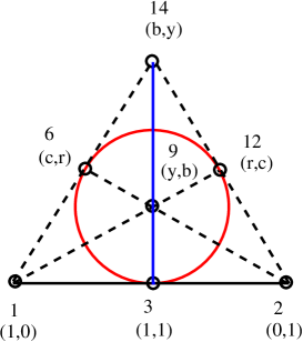
Figure 1: The “kernel of entanglement” for two-qubit systems as a pencil of lines (one represented by the circle) in the Fano plane. The points of the configuration correspond to the nontrivial observables of equation (19). The extra labelling refers to the points of the projective line of $GF(2)^{\otimes 3}$ (see Section 4.2).

  

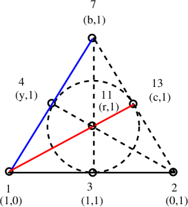
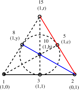
Figure 2: Two pencils of lines reproducing the product rules of the observables given Table 3. The points, apart from 1 to 3, are now the observables from (20). The extra labelling refers again to the points of the projective line over $GF(2)^{\otimes 3}$ (see Section 4.2).

There exists an equivalence between the unbiasedness of sets of bases and particular sets of mutually commuting operators sharing a base of eigenvectors. Let us consider the partitioning of the $15$ observables attached to two spin-$\frac{1}{2}$ particles into the following $5$ $(=4+1)$ mutually unbiased sets arranged in rows [17]

$$\begin{array}[]{ccc}1_{2}\otimes\sigma_{z}&\sigma_{z}\otimes 1_{2}&\sigma_{z}\otimes\sigma_{z}\\ \sigma_{x}\otimes 1_{2}&1_{2}\otimes\sigma_{y}&\sigma_{x}\otimes\sigma_{y}\\ \sigma_{x}\otimes\sigma_{z}&\sigma_{z}\otimes\sigma_{x}&\sigma_{y}\otimes\sigma_{y}\\ 1_{2}\otimes\sigma_{x}&\sigma_{y}\otimes 1_{2}&\sigma_{y}\otimes\sigma_{x}\\ \sigma_{y}\otimes\sigma_{z}&\sigma_{x}\otimes\sigma_{x}&\sigma_{z}\otimes\sigma_{y}\\ \end{array}=\begin{array}[]{ccc}1&2&3\\ 4&5&6\\ 7&8&9\\ 10&11&12\\ 13&14&15\\ \end{array}$$ (11)

where $1_{2}$ is the $2\times 2$ unit matrix and $\sigma_{x}$, $\sigma_{y}$ and $\sigma_{z}$ are the classical Pauli matrices. All the observables in (11) have doubly-degenerate eigenvalues, $\pm 1$, and each row gives rise to an orthogonal base; the bases represented by the 3rd and 5th rows are entangled. Every operator in a row is the product of the other two, i.e. $1*2=3$, $4*5=6,\ldots$ (here $*$ stands for the matrix product), but no similar rule seems to exist between operators in two different rows. The $3\times 3$ arrays of observables of Mermin’s type, mentioned in the introduction, are of the following forms

$$\begin{array}[]{ccccccccccccccccccc}1&2&3&\mbox{}&\mbox{}&1&2&3&\mbox{}&\mbox{}&1&4&7&\mbox{}&\mbox{}&1&11&13&\\ 4&10&14&\mbox{}&\mbox{}&13&15&14&\mbox{}&\mbox{}&2&5&15&\mbox{}&\mbox{}&2&10&8&\\ 7&8&9&\mbox{}&\mbox{}&11&5&9&\mbox{}&\mbox{}&3&6&12&\mbox{}&\mbox{}&3&12&6&\\ \end{array}$$ (15)

In each of the above arrays, the observables in every row or column are mutually commuting, each being the product of the other two except for the last column where a minus sign appears, i.e., $3*14=-9$; the product of the three operators in each row and the first two columns thus yields $+1_{2}$, whereas for the third column it is $-1_{2}$. In view of our subsequent considerations it is useful to enumerate the orthogonal bases attached to rows and columns of the first Mermin square on the left-hand side of equation (15), omitting, for the sake of simplicity, a normalization factor and denoting the sign of eigenvalues of the corresponding operators by subscripts:

$$\begin{array}[]{ccccc}[1,2,3]:&(1,0,0,0)_{+++}&(0,1,0,0)_{-+-}&(0,0,1,0)_{+--}&(0,0,0,1)_{--+}\\ =&|00\rangle&|01\rangle&|10\rangle&|11\rangle\\ [4,10,14]:&(1,1,1,1)_{+++}&(1,-1,1,-1)_{+--}&(1,1,-1,-1)_{-+-}&(1,-1,-1,1)_{--+}\\ [7,8,9]:&(1,1,1,-1)_{+++}&(1,-1,1,1)_{+--}&(1,1,-1,1)_{-+-}&(1,-1,-1,-1)_{--+}\\ [1,4,7]:&(1,0,1,0)_{+++}&(1,0,-1,0)_{+--}&(0,1,0,1)_{-+-}&(0,1,0,-1)_{--+}\\ [2,10,8]:&(1,1,0,0)_{+++}&(1,-1,0,0)_{+--}&(0,0,1,1)_{-+-}&(0,0,1,-1)_{--+}\\ [3,14,9]:&(1,0,0,1)_{++-}&(1,0,0,-1)_{+-+}&(0,1,1,0)_{-++}&(0,-1,1,0)_{---}\\ =&|00\rangle+|11\rangle&|00\rangle-|11\rangle&|01\rangle+|10\rangle&|01\rangle-|10\rangle\\ \end{array}\!$$

For the first two arrays of (15), an orthogonal base of the Bell states is associated with the third column; for the other two squares, the Bell states are carried by the operators in the third row as follows

$$\begin{array}[]{ccccc}[3,6,12]:&(1,0,0,i)_{+++}&(1,0,0,-i)_{+--}&(0,1,i,0)_{-++}&(0,1,-i,0)_{---}\\ =&|00\rangle+i|11\rangle&|00\rangle-i|11\rangle&|01\rangle+i|10\rangle&|01\rangle-i|10\rangle\\ \end{array}$$

3 Algebra and geometry of two spin-$\boldsymbol{\frac{1}{2}}$ particles

The four different representations of Mermin’s square, equation (15), give us important hints about the existence of an underlying algebraic geometrical principle governing interaction of two spin-$\frac{1}{2}$ particles. The base line $(1,2,3)$ is common to all the four arrays, each of the remaining operators from $4$ to $15$ appears twice, and the (Bell) entangled triples $(3,14,9)$ and $(3,6,12)$ form a column and a row, respectively. Our goal in this section is to reveal this hidden geometry.

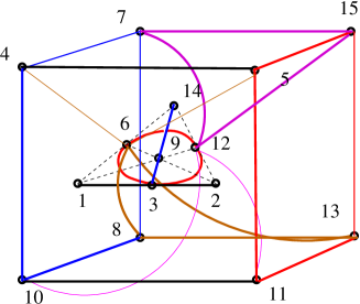
Figure 3: A geometry of a system of two spin-$\frac{1}{2}$ particles. The “inner” observables are arranged as shown in Fig. 1, whereas the “outer” ones form a cubic configuration. A couple of “inner” observables commute with eight “outer” ones forming two “complementary” four-tuples. They exist three such pairs: $(6,12)$, $(9,14)$ and $(1,2)$. The “inner/outer” relation is, however, illustrated for the first pair only. The concerned triples of observables which are entangled are represented with thicker lines.

To this end in view, we first add to the set given by equation (11) the identity operator $0\equiv 1_{2}\otimes 1_{2}$, obtaining

$$\mathcal{S}=\{0,1,2,\ldots,15\},$$ (18)

and partition this set into two subsets $\mathcal{A}$ and $\mathcal{B}$, where

$$\mathcal{A}=\{0,1,2,3,6,9,12,14\}$$ (19)

comprises the “computational” operators $\mathcal{C}=\{0,1,2,3\}$ and the “entangled” operators $\mathcal{E}=\{6,9,12,14\}$, and

$$\mathcal{B}=\{4,5,7,8,10,11,13,15\},$$ (20)

which can also be partitioned into two subsets of cardinality four as shown in Table 3. Next we create the multiplication tables for the elements of $\mathcal{A}$ (Table 3), $\mathcal{B}$ (Table 3) and those of both sets (Table 3) in order to see that the following properties hold for two observables $O$ and $O^{\prime}$

$$O,O^{\prime}\in\mathcal{A}~{}~{}{\rm or}~{}~{}O,O^{\prime}\in\mathcal{B}~{}~{}\Rightarrow~{}~{}O*O^{\prime}\in\mathcal{A},$$

$$O\in\mathcal{A}~{}~{}{\rm and}~{}~{}O^{\prime}\in\mathcal{B}~{}~{}\Rightarrow~{}~{}O*O^{\prime}\in\mathcal{B}.$$

One immediately recognizes that the multiplication table of $\mathcal{C}$ is, except for a factor $-1$ or $\pm i$, isomorphic to the addition table of the Galois field $GF(4)\cong GF(2)[x]/\langle x^{2}+x+1\rangle$ and that of $\mathcal{A}$ to the addition table of the Galois field $GF(8)\cong GF(2)[x]/\langle x^{3}+x+1\rangle$. The set $GF(8)^{*}\equiv GF(8)\setminus\{0\}$ is a cyclic group generated by a single element and its representation in terms of $3$-tuples in $GF(2)^{\otimes 3}$ provides the coordinates of seven points of the projective plane of order two, the Fano plane [18]. Hence, we can identify the elements of the set $\mathcal{A}$, omitting the trivial one (0), with the points of such a plane and obtain the configuration shown in Fig. 1. In this figure, three operators are on a line if and only if the product of two of them equals, again apart from a factor $-1$ or $\pm i$, the remaining one (see Table 3), with the understanding that full/broken lines join commuting/non-commuting operators. The three full lines, distinguished from each other by different colours, form a so-called pencil, i.e., the set of lines passing through the same point, called the base point – see, e.g., [11], and, in this particular case, each of them is endowed with the triple of operators carrying Bell states. The essence of quantum entanglement between two spin-$\frac{1}{2}$ particles is thus embodied in a very simple geometry! If, furthermore, the set $\mathcal{B}$ and Table 3 are taken into account, we get two analogous configurations, as depicted in Fig. 2. However, these configurations differ crucially from the first one as any full line in either of them contains triples of operators that share an unentangled orthogonal base of eigenvectors. All in all, the fifteen operators 1 to 15 are thus found to form a remarkable configuration comprising the seven elements of the kernel of Fig. 1 and the ten elements of the “outer shell” forming a cube, as shown in Fig. 3.

4 Entanglement and finite ring geometry

4.1 The $\boldsymbol{GF(2)^{\otimes 2}}$ geometry of the Mermin square

The remarkable algebraic geometrical properties of a system of two spin-$\frac{1}{2}$ particles discussed in the previous section can be given a more appropriate setting if we employ the concept of projective geometry over rings, in particular that of projective lines defined over finite rings. The most prominent, and at first sight counterintuitive, feature of ring geometries (of dimension two and higher) is the fact that two distinct points/lines need not to have a unique connecting line/meeting point [19, 22]. As a result, such geometries feature new concepts like neighbour and distant, which turns out to be relevant for our geometrical interpretation of mutual unbiasedness, complementarity and non-locality in quantum physics. All these features are intimately connected with the structure of the set of zero divisors of the ring. As this kind of geometry has until recently been virtually unknown to the physics community, we shall start from scratch and recollect first some basic definitions, concepts and properties of rings (see, e.g., [23, 24, 25]).

A ring is a set $R$ (or, more specifically, ($R,+,\times$)) with two binary operations, usually called addition ($+$) and multiplication ($\times$), such that $R$ is an Abelian group under addition and a semigroup under multiplication, with multiplication being both left and right distributive over addition. A ring in which the multiplication is commutative is a commutative ring. A ring $R$ with a multiplicative identity 1 such that 1$r$ = $r$1 = $r$ for all $r\in R$ is a ring with unity. A ring containing a finite number of elements is a finite ring. In what follows the word ring will always mean a commutative ring with unity. An element $r$ of the ring $R$ is a unit (or an invertible element) if there exists an element $r^{-1}$ such that $rr^{-1}=r^{-1}r=1$. The element $r^{-1}$, uniquely determined by $r$, is called the multiplicative inverse of $r$. The set of units forms a group under multiplication. A (non-zero) element $r$ of $R$ is said to be a (non-trivial) zero-divisor if there exists $s\neq 0$ such that $sr=rs=0$. An element of a finite ring is either a unit or a zero-divisor. A ring in which every non-zero element is a unit is a field; finite (or Galois) fields, often denoted by $GF(q$), have $q$ elements and exist only for $q=p^{n}$, where $p$ is a prime number and $n$ a positive integer. The smallest positive integer $s$ such that $s1=0$, where $s1$ stands for $1+1+1+\cdots+1$ ($s$ times), is called the characteristic of $R$; if $s1$ is never zero, $R$ is said to be of characteristic zero. An ideal ${\cal I}$ of $R$ is a subgroup of $(R,+)$ such that $a{\cal I}={\cal I}a\subset{\cal I}$ for all $a\in R$. An ideal of the ring $R$ which is not contained in any other ideal but $R$ itself is called a maximal ideal. If an ideal is of the form $Ra$ for some element $a$ of $R$ it is called a principal ideal, usually denoted by $\langle a\rangle$. A ring with a unique maximal ideal is a local ring. Let $R$ be a ring and ${\cal I}$ one of its ideals. Then $\overline{R}\equiv R/{\cal I}=\{a+{\cal I}~{}|~{}a\in R\}$ together with addition $(a+{\cal I})+(b+{\cal I})=a+b+{\cal I}$ and multiplication $(a+{\cal I})(b+{\cal I})=ab+{\cal I}$ is a ring, called the quotient (or factor) ring of $R$ with respect to ${\cal I}$; if ${\cal I}$ is maximal, then $\overline{R}$ is a field. A very important ideal of a ring is that one represented by the intersection of all maximal ideals; this ideal is called the Jacobson radical. Finally, we mention a couple of relevant examples of rings: a polynomial ring, $R[x]$, viz. the set of all polynomials in one variable $x$ and with coefficients in the ring $R$, and the ring $R_{\otimes}$ that is a (finite) direct product of rings, $R_{\otimes}\equiv R_{1}\otimes R_{2}\otimes\cdots\otimes R_{n}$, where both addition and multiplication are carried out componentwise and where the individual rings need not be the same.

Given a ring $R$ with unity, the general linear group of invertible 2$\times$2 matrices with entries in $R$, a pair ($\alpha,\beta$) $\in R^{2}$ is called admissible over $R$ if there exist $\gamma,\delta\in R$ such that [26]

$$\left(\begin{array}[]{cc}\alpha&\beta\\ \gamma&\delta\\ \end{array}\right)\in{\rm GL}(2,R).$$ (23)

The projective line over $R$, denoted as $PR(1)$, is defined as the set of classes of ordered pairs $(\varrho\alpha,\varrho\beta)$, where $\varrho$ is a unit and $(\alpha,\beta)$ is admissible [22, 26, 27, 28, 29]. Such a line carries two non-trivial, mutually complementary relations of neighbour and distant. In particular, its two distinct points $X$:=$(\varrho\alpha,\varrho\beta)$ and $Y$:=$(\varrho\gamma,\varrho\delta)$ are called neighbour (or, parallel) if

$$\left(\begin{array}[]{cc}\alpha&\beta\\ \gamma&\delta\\ \end{array}\right)\notin{\rm GL}(2,R)$$ (26)

and distant otherwise, i.e., if condition (23) is met. The neighbour relation is reflexive (every point is obviously neighbour to itself) and symmetric (i.e., if $X$ is neighbour to $Y$ then $Y$ is neighbour to $X$ too), but, in general, not transitive (i.e., $X$ being neighbour to $Y$ and $Y$ being neighbour to $Z$ does not necessarily mean that $X$ is neighbour to $Z$ – see, e.g., [22, 26, 29]). Given a point of $PR(1)$, the set of all neighbour points to it will be called its neighbourhood. For a finite commutative ring $R$, equation (23) reads

$$\det\left(\begin{array}[]{cc}\alpha&\beta\\ \gamma&\delta\\ \end{array}\right)\in R^{*},$$ (29)

and equation (26) reduces to

$$\det\left(\begin{array}[]{cc}\alpha&\beta\\ \gamma&\delta\\ \end{array}\right)\in R\backslash R^{*},$$ (32)

where $R^{*}$ denotes the set of units (invertible elements) and $R\backslash R^{*}$ stands for the set of zero-divisors of $R$ (including the trivial zero divisor 0). Obviously, if $R$ is a field then ‘neighbour’ simply reduces to ‘identical’ and ‘distant’ to ‘different’; for given the fact that 0 is the only zero-divisor in a field, equation (32) reduces to $\alpha\delta-\gamma\beta=0$, which indeed implies that $(\gamma,\delta)=(\varrho\alpha,\varrho\beta)$.

Table 4: Addition and multiplication in $R_{\perp}$ (top) and in $GF(4)\simeq GF(2)[x]/\langle x^{2}+x+1\rangle$ (bottom).

$+$	$0$	$1$	$x$	$x+1$
$0$	$0$	$1$	$x$	$x+1$
$1$	$1$	$0$	$x+1$	$x$
$x$	$x$	$x+1$	$0$	$1$
$x+1$	$x+1$	$x$	$1$	$0$

$\times$	$0$	$1$	$x$	$x+1$
$0$	$0$	$0$	$0$	$0$
$1$	$0$	$1$	$x$	$x+1$
$x$	$0$	$x$	$x$	$0$
$x+1$	$0$	$x+1$	$0$	$x+1$

$+$	$0$	$1$	$x$	$x+1$
$0$	$0$	$1$	$x$	$x+1$
$1$	$1$	$0$	$x+1$	$x$
$x$	$x$	$x+1$	$0$	$1$
$x+1$	$x+1$	$x$	$1$	$0$

$\times$	$0$	$1$	$x$	$x+1$
$0$	$0$	$0$	$0$	$0$
$1$	$0$	$1$	$x$	$x+1$
$x$	$0$	$x$	$x+1$	$1$
$x+1$	$0$	$x+1$	$1$	$x$

To illustrate the concept, and to meet the first relevant example of ring geometry in quantum theory, we shall consider the projective line defined over the ring of Galois double numbers $R_{\perp}\equiv GF(2)^{\otimes 2}$ [12]. The ring $R_{\perp}$ is of characteristic two and consists of the four elements $0$, $1$, $x$, $x+1$ subject to the addition and multiplication rules given in Table 4, as it can readily be verified from its isomorphism to the quotient ring $GF(2)[x]/\langle x^{2}-x\rangle$ [20]; it is important to realize at this point that although the addition table of $R_{\perp}$ is the same as that of the corresponding Galois field, $GF(4)\cong GF(2)[x]/\langle x^{2}+x+1\rangle$ (compare the left-hand sides of Table 4), the two rings substantialy differ in their multiplication tables (the right-hand sides of Table 4), because $GF(4)$, like any field, does not possess any non-trivial zero-divisors. As ‘1’ is the only unit of $R_{\perp}$, from equation (29) we find that the associated projective line, $PR_{\perp}(1)$, features altogether nine points out of which (i) seven points are represented by pairs where at least one entry is a unit, namely

$$(1,0),\ (1,x),\ (1,x+1),\ (1,1),$$

$$(0,1),\ (x,1),\ (x+1,1),$$

and (ii) two points have both coordinate entries zero-divisors, not of the same ideal, viz.

$$(x,x+1),\ (x+1,x).$$

To reveal the fine structure of the line we pick up three distinguished points $U$:=$(1,0)$, $V$:=$(0,1)$ and $W$:=$(1,1)$, representing nothing but the ordinary projective line of order two embedded in $PR_{\perp}(1)$, which are obviously pairwise distant and whose neighbourhoods are readily found to read

$$U:\ \ (1,x),\ (1,x+1),\ (x,x+1),\ (x+1,x),$$

$$V:\ \ (x,1),\ (x+1,1),\ (x,x+1),\ (x+1,x),$$

$$W:\ \ (1,x),\ (1,x+1),\ (x,1),\ (x+1,1).$$

Now, as the coordinate system on this line can always be chosen in such a way that the coordinates of any three mutually distant points are made identical to those of $U$, $V$ and $W$, from the last three expressions we discern that the neighbourhood of any point of the line features four distinct points, the neighbourhood of any two distant points have two points in common (which makes the neighbour relation non-transitive) and the neighbourhoods of any three mutually distant points have no element in common. The nine points of the line $PR_{\perp}(1)$ can thus be arranged into a $3\times 3$ array as shown in Fig. 4 (see also Fig. 2 of Ref. [21] for a different, “conic” representation of $PR_{\perp}$). This array has an important property that all the points in the same row and/or column are pairwise distant. Moreover, a closer look at Fig. 3 reveals that one triple of mutually distant points, that located in the third (blue) column, differs from all others in having both coordinates of all the three points of the same character, namely either zero-divisors (the points $(x,x+1)$ and $(x+1,x))$, or units (the point $(1,1)$). After identifying, in an obvious way, the observables of the first (or the second) Mermin square in (15) with the points of $PR_{\perp}(1)$, one immediately sees that the concept mutually commuting translates ring geometrically into mutually distant and that the “Bell-borne” specific character of the observables of the third column has its geometrical counterpart in the above-mentioned distinguishing properties of the coordinates of the corresponding points.

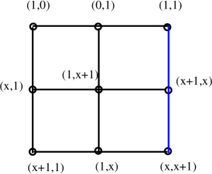
Figure 4: An illustration of the structure of the projective line over $R_{\perp}$. If two distinct points are joined by a line, they are distant; if not, they are neighbour.

4.2 The three pencil configurations and the projective line over $\boldsymbol{GF(2)^{\otimes 3}}$

Table 5: Addition and multiplication in $R_{\triangle}$.

$+$	$0$	$1$	$b$	$y$	$r$	$c$	$g$	$m$
$0$	$0$	$1$	$b$	$y$	$r$	$c$	$g$	$m$
$1$	$1$	$0$	$y$	$b$	$c$	$r$	$m$	$g$
$b$	$b$	$y$	$0$	$1$	$m$	$g$	$c$	$r$
$y$	$y$	$b$	$1$	$0$	$g$	$m$	$r$	$c$
$r$	$r$	$c$	$m$	$g$	$0$	$1$	$y$	$b$
$c$	$c$	$r$	$g$	$m$	$1$	$0$	$b$	$y$
$g$	$g$	$m$	$c$	$r$	$y$	$b$	$0$	$1$
$m$	$m$	$g$	$r$	$c$	$b$	$y$	$1$	$0$

$\times$	$0$	$1$	$b$	$y$	$r$	$c$	$g$	$m$
$0$	$0$	$0$	$0$	$0$	$0$	$0$	$0$	$0$
$1$	$0$	$1$	$b$	$y$	$r$	$c$	$g$	$m$
$b$	$0$	$b$	$b$	$0$	$0$	$b$	$0$	$b$
$y$	$0$	$y$	$0$	$y$	$r$	$g$	$g$	$r$
$r$	$0$	$r$	$0$	$r$	$r$	$0$	$0$	$r$
$c$	$0$	$c$	$b$	$g$	$0$	$c$	$g$	$b$
$g$	$0$	$g$	$0$	$g$	$0$	$g$	$g$	$0$
$m$	$0$	$m$	$b$	$r$	$r$	$b$	$0$	$m$

The above-established mutually commuting – mutually distant analogy can be extended to a more general ring geometrical setting, that of the projective line defined over $R_{\triangle}\equiv GF(2)^{\otimes 3}$ [21]. The ring $R_{\triangle}$, of characteristic two and cardinality eight, comprises the unity $[1,1,1]\equiv 1$, the trivial zero-divisor $[0,0,0]\equiv 0$, and six other zero-divisors forming three pairs, namely $[1,0,0]\equiv b$ and $[0,1,1]\equiv y$, $[0,1,0]\equiv r$ and $[1,0,1]\equiv c$, $[0,0,1]\equiv g$ and $[1,1,0]\equiv m$; the entries in each pair are complementary in the sense that they sum to the unity. The elements of the ring are subject to the addition and multiplication properties as shown in Table 5, from where it follows that the ring has three maximal – and principal as well – ideals

$$\langle y\rangle=\{0,r,g,y\},\quad\langle c\rangle=\{0,b,g,c\}\quad\mbox{and}\quad\langle m\rangle=\{0,b,r,m\},$$

and three other principal ideals

$$\langle b\rangle=\{0,b\}=\langle c\rangle\cap\langle m\rangle,\quad\langle r\rangle=\{0,r\}=\langle y\rangle\cap\langle m\rangle\quad\mbox{and}\quad\langle g\rangle=\{0,g\}=\langle y\rangle\cap\langle c\rangle.$$

By making use of these facts, the associated projective line, $PR_{\triangle}(1)$, is found to consist of the following twenty-seven points [21]: (i) the three distinguished points (the “nucleus”),

$$(1,0),\qquad(0,1),\quad\mbox{and}\quad(1,1),$$

which represent the ordinary projective line over $GF(2)$ embedded in $PR_{\triangle}(1)$; (ii) six pairs of points of the “inner shell” whose coordinates feature both the unity and a zero-divisor,

$$(1,b),(b,1);\quad(1,y),(y,1);\quad\ldots;$$

and (iii) six pairs of points of the “outer shell” whose coordinates have zero-divisors in both the entries,

$$(b,y),(y,b);\quad\ldots;\quad(c,y),(y,c);\quad\ldots;$$

which were split into two groups according to as both entries are composite zero-divisors or not.

The fine structure of this line has thoroughly been investigated in [21] and the most relevant results are here reproduced in Tables 6 to 9, using the notation of Ref. [21]. After identifying the points of the line with the observables as shown in Figs. 1 and 2, from Tables 3 and 3 we find out that the subsets in question provide a perfect match for the geometry of all the three pencils. The picture, however, is not complete as one readily realizes when trying, under the given correspondence, to reproduce Tables 3 and 3; in the former case we see that the two pictures differ in four places (Table 8), whilst in the latter case in as many as fourteen entries (Table 9)!

Table 6: A subset of $PR_{\triangle}(1)$ whose distant/neighbour ($+/-$) relations exactly reproduce the commutation relations embodied in the “entangled” pencil of lines shown in Fig. 1.

	$(1,0)$	$(0,1)$	$(1,1)$	$(c,r)$	$(b,y)$	$(y,b)$	$(r,c)$
$(1,0)$	$-$	$+$	$+$	$-$	$-$	$-$	$-$
$(0,1)$	$+$	$-$	$+$	$-$	$-$	$-$	$-$
$(1,1)$	$+$	$+$	$-$	$+$	$+$	$+$	$+$
$(c,r)$	$-$	$-$	$+$	$-$	$-$	$-$	$+$
$(b,y)$	$-$	$-$	$+$	$-$	$-$	$+$	$-$
$(y,b)$	$-$	$-$	$+$	$-$	$+$	$-$	$-$
$(r,c)$	$-$	$-$	$+$	$+$	$-$	$-$	$-$

Table 7: A subset of $PR_{\triangle}(1)$ whose distant/neighbour relations match the commutation relations exhibited by the “unentangled” pencil of lines shown in Fig. 2, left; the identical table is obtained if we exchange the order of coordinates, which fits the geometry of the pencil of Fig. 2, right.

	$(1,0)$	$(0,1)$	$(1,1)$	$(y,1)$	$(b,1)$	$(c,1)$	$(r,1)$
$(1,0)$	$-$	$+$	$+$	$+$	$+$	$+$	$+$
$(0,1)$	$+$	$-$	$+$	$-$	$-$	$-$	$-$
$(1,1)$	$+$	$+$	$-$	$-$	$-$	$-$	$-$
$(y,1)$	$+$	$-$	$-$	$-$	$+$	$-$	$-$
$(b,1)$	$+$	$-$	$-$	$+$	$-$	$-$	$-$
$(c,1)$	$+$	$-$	$-$	$-$	$-$	$-$	$+$
$(r,1)$	$+$	$-$	$-$	$-$	$-$	$+$	$-$

Table 8: A subset of $PR_{\triangle}(1)$ that is the best match for the geometry of the observables given in Table 3; the two configurations differ in four places indicated by an exclamation mark.

	$(y,1)$	$(b,1)$	$(r,1)$	$(c,1)$	$(1,c)$	$(1,b)$	$(1,r)$	$(1,y)$
$(y,1)$	$-$	$+$	$-$	$-$	$-$!	$+$	$-$	$-$
$(b,1)$	$+$	$-$	$-$	$-$	$-$	$-$	$+$	$+$
$(r,1)$	$-$	$-$	$-$	$+$	$+$	$+$	$-$	$-$
$(c,1)$	$-$	$-$	$+$	$-$	$-$	$-$	$+$	$-!$
$(1,c)$	$-!$	$-$	$+$	$-$	$-$	$-$	$+$	$-$
$(1,b)$	$+$	$-$	$+$	$-$	$-$	$-$	$-$	$+$
$(1,r)$	$-$	$+$	$-$	$+$	$+$	$-$	$-$	$-$
$(1,y)$	$-$	$+$	$-$	$-!$	$-$	$+$	$-$	$-$

Table 9: A subset of $PR_{\triangle}(1)$ that is the best match for the geometry of the observables given in Table 3; the two configurations differ in fourteen places indicated by an exclamation mark.

	$(1,0)$	$(0,1)$	$(1,1)$	$(c,r)$	$(b,y)$	$(y,b)$	$(r,c)$
$(y,1)$	$+$	$-$	$-$	$+$	$+$	$-$	$-$
$(b,1)$	$+$	$-$	$-$	$-$	$-$	$+$	$-!$
$(r,1)$	$+$	$-$	$-$	$+!$	$-$	$-!$	$-!$
$(c,1)$	$+$	$-$	$-$	$-!$	$-!$	$+!$	$+!$
$(1,c)$	$-$	$+$	$-$	$+$	$+!$	$-!$	$-$
$(1,b)$	$-$	$+$	$-$	$-$	$+$	$-$	$-!$
$(1,r)$	$-$	$+$	$-$	$-$	$-!$	$-$	$+$
$(1,y)$	$-$	$+$	$-$	$-!$	$-$	$+$	$+!$

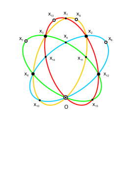
Figure 5: The structure and mutual relation between the four maximal ideals, represented by points of four distinct ellipses, of $R_{\diamond}$.

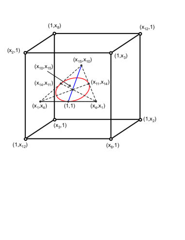
Figure 6: Two distinct subsets of $PR_{\diamondsuit}(1)$ reproducing the structure of both the kernel and the shell of the full configuration of observables characterizing two-qubit systems. Unfortunately, this framework is insufficient to harbour the coupling between the two objects (compare with Fig. 3).

4.3 Towards a fuller picture: the projective line over $\boldsymbol{GF(2)^{\otimes 4}}$

These last observations clearly indicate that higher order rings have to be employed to obtain a satisfactory picture of the behaviour of two spin-$\frac{1}{2}$ particles. As an important intermediate step to reach this goal seems to be the structure of the projective line defined over $R_{\diamondsuit}\equiv GF(2)^{\otimes 4}$.

We will not go into much detail here and simply observe that the 16 elements of $R_{\diamondsuit}$ can be represented in the following form

$$x_{0}=[0,0]\equiv 0,\quad x_{1}=[0,1],\quad x_{2}=[0,a],\quad x_{3}=[0,b],$$

$$x_{4}=[1,0],\quad x_{5}=[1,1]\equiv 1,\quad x_{6}=[1,a],\quad x_{7}=[1,b],$$

$$x_{8}=[a,0],\quad x_{9}=[a,1],\quad x_{10}=[a,a],\quad x_{11}=[a,b],$$

$$x_{12}=[b,0],\quad x_{13}=[b,1],\quad x_{14}=[b,a],\quad x_{15}=[b,b].$$

which stems from the fact that $R_{\diamondsuit}\cong R_{\perp}\otimes R_{\perp}$ and from the representation of $R_{\perp}$ given in Section 4.1 after identifying $a=x$ and $b=x+1$. The fifteen zero-divisors of $R_{\diamondsuit}$ form four maximal ideals, whose composition and mutual relation are depicted in Fig. 5. Although yielding the trivial Jacobson radical ($\{x_{0}\}$), any triple of them share one more element, and there are altogether four such distinguished elements: $x_{2}$, $x_{3}$, $x_{8}$ and $x_{12}$. The associated projective line, $PR_{\diamondsuit}(1)$, is easily found to contain subsets whose properties reproduce properly not only those of Mermin’s squares (like $PR_{\perp}(1)$) and of the three pencil-borne geometries (like $PR_{\triangle}(1)$), but also a subset which accounts for the behaviour of the observables forming the “outer” shell (the cube) in Fig. 3. This particular subset consists of eight points whose coordinates feature the unity and one of the above-mentioned distinguished zero-divisors, as illustrated in Fig. 6. So, the structure of $PR_{\diamondsuit}(1)$ is a proper ring geometrical setting for the observables of both the “inner” and “outer” shells when considered separately. Yet, it fails to provide a correct picture for the coupling between the two shells, because it implies that no observable from one shell commutes with any observable from the other one, which is clearly not the case. To glue the two pictures thus clearly necessitates to look at projective lines over higher order, and possibly non-commutative rings and/or allied algebras.

5 Conclusion

The fifteen observables/operators characterizing the interaction of two spin-$\frac{1}{2}$ particles were found to exhibit two distinct, yet intimately connected, algebraic geometrical structures, considered first as points of the ordinary projective plane of order two and then as points of projective lines defined over $GF(2)^{\otimes n}$, with $n=2,3$ and 4. In the first picture, the observables are regarded as three pencils of lines. These pencil-configurations, each featuring seven points, share a line, and a line in any of them comprises three observables. All the lines in each pencil carry mutually commuting operators; in one of the pencils, which we call the kernel, the observables on two lines share a base of Bell states. The three operators on any line in each pencil represent a row or column of some Mermin’s “magic” square. An inherent geometrical nature of Mermin’s squares is shown to be captured by the structure of the projective line defined over $GF(2)^{\otimes 2}$, that of all the three pencils, when taken together, by the line over $GF(2)^{\otimes 3}$, whereas the behavior of the kernel and its complement (the cube-shell), when considered separately, is reproduced by the properties of the line over $GF(2)^{\otimes 4}$. To complete the picture, it just remains to find a ring line, or a very similar object, that would also account for the coupling between the kernel and its complement.

To close this paper, a group-theoretical comment is in order. For $N$ qubits, the Lie group $U(2^{N})$ and the chain $U(2^{N})\supset SU(2^{N})$ play an important role. According to a theorem credited to Racah [32], for a semi-simple Lie group $G$ of order $r$ and rank $l$, a complete set of $\frac{1}{2}(r+l)$ commuting operators can be constructed in the enveloping algebra of $G$. For $N=2$ qubits ($d=2^{2}$), the relevant group is $SU(4)$ for which $r=d^{2}-1=15$ and $l=d-1=3$. In this case, we have $\frac{r}{l}=d+1=5$ MUBs corresponding to a set of $l=d-1=3$ commuting operators taken from a complete, with respect to $SU(4)$, set of $\frac{1}{2}(r+l)=\frac{1}{2}(d-1)(d+2)=9$ operators. These matters are presently the object of our investigations (see also [33]).

Acknowledgements

This work was partially supported by the Science and Technology Assistance Agency under the contract $\#$ APVT–51–012704, the VEGA project $\#$ 2/6070/26 (both from Slovak Republic) and by the trans-national ECO-NET project $\#$ 12651NJ “Geometries Over Finite Rings and the Properties of Mutually Unbiased Bases” (France). We are grateful to Dr. Petr Pracna for a number of fruitful comments/remarks and for creating the last two figures. One of the authors (M.S.) would like to thank the warm hospitality extended to him by the Institut FEMTO-ST in Besançon and the Institut de Physique Nucléaire in Lyon.

References

- [1] Einstein A., Podolsky B., Rosen N., Can quantum-mechanical description of physical reality be considered complete?, Phys. Rev., 1935, V.47, 777–780.
- [2] Bohm D., Quantum theory, New York, Prentice Hall, 1951.
- [3] Bell J.S., On the problem of hidden variables in quantum mechanics, Rev. Modern Phys., 1966, V.38, 447–452.
- [4] Kochen S., Specker E.P., The problem of hidden variables in quantum mechanics, J. Math. Mech., 1976, V.17, 59–88.
- [5] Peres A., Incompatible results of quantum measurements, Phys. Lett. A, 1990, V.151, 107–108.
- [6] Mermin N.D., Hidden variables and two theorems of John Bell, Rev. Modern Phys., 1993, V.65, 803–815.
- [7] Aspect A., Grangier P., Roger G., Experimental tests of Bell’s inequalities using time-varying analyzers, Phys. Rev. Lett., 1982, V.49, 1804–1807.
- [8] Schrödinger E., Discussion of probability relations between separated systems, Proc. Cambridge Phil. Soc., 1935, V.31, 555–563, 1936, V.32, 446–451.
- [9] Peres A., Quantum theory: concepts and methods, Dordrecht, Kluwer Academic Publishers, 1998.
- [10] Bohr N., Can quantum-mechanical description of physical reality be considered complete?, Phys. Rev., 1935, V.48, 696–702.
- [11] Polster B., A geometrical picture book, New York, Springer, 1998.
- [12] Saniga M., Planat M., Minarovjech M., The projective line over the finite quotient ring and quantum entanglement II. The Mermin “magic” square/pentagram, quant-ph/0603206.
- [13] Aravind P.K., Quantum mysteries revisited again, Amer. J. Phys., 2004, V.72, 1303–1307.
- [14] Planat M., Rosu H., Mutually unbiased phase states, phase uncertainties and Gauss sums, Eur. Phys. J. D At. Mol. Opt. Phys., 2005, V.36, 133–139, quant-ph/0506128.
- [15] Saniga M., Planat M., Rosu H., Mutually unbiased bases and finite projective planes, J. Opt. B Quantum Semiclass. Opt., 2004, V.6, L19–L20, math-ph/0403057.
- [16] Kibler M.R., Planat M., A SU(2) recipe for mutually unbiased bases, Internat. J. Modern Phys. B, 2006, V.20, 1802–1807, quant-ph/0601092.
- [17] Lawrence J., Brukner C., Zeilinger A., Mutually unbiased binary observables sets on qubits, Phys. Rev. A, 2002, V.65, 032320, 5 pages, quant-ph/0104012.
- [18] Planat M., Saniga M., Abstract algebra, projective geometry and time encoding of quantum information, in Proceedings of the ZiF Workshop “Endophysics, Time, Quantum and the Subjective” (January 17–22, 2005, Bielefeld), Editors R. Buccheri, A.C. Elitzur and M. Saniga, Singapore, World Scientific Publishing, 2005, 121–138, quant-ph/0503159.
- [19] Saniga M., Planat M., Projective planes over “Galois” double numbers and a geometrical principle of complementarity, Chaos Solitons Fractals, 2006, in press, math.NT/0601261.
- [20] Saniga M., Planat M., The projective line over the finite quotient ring GF(2)[]/ and quantum entanglement I. Theoretical background, quant-ph/0603051.
- [21] Saniga M., Planat M., On the fine structure of the projective line over , math.AG/0604307.
- [22] Veldkamp F.D., Geometry over rings, in Handbook of Incidence Geometry, Editor F. Buekenhout, Amsterdam, Elsevier, 1995, 1033–1084.
- [23] Fraleigh J.B., A first course in abstract algebra, 5th ed., Reading (MA), Addison-Wesley, 1994, 273–362.
- [24] McDonald B.R., Finite rings with identity, New York, Marcel Dekker, 1974.
- [25] Raghavendran R., Finite associative rings, Compos. Math., 1969, V.21, 195–229.
- [26] Herzer A., Chain geometries, in Handbook of Incidence Geometry, Editor F. Buekenhout, Amsterdam, Elsevier, 1995, 781–842.
- [27] Blunck A., Havlicek H., Projective representations I: Projective lines over a ring, Abh. Math. Sem. Univ. Hamburg, 2000, V.70, 287–299.
- [28] Blunck A., Havlicek H., Radical parallelism on projective lines and non-linear models of affine spaces, Math. Pannon., 2003, V.14, 113–127.
- [29] Havlicek H., Divisible designs, Laguerre geometry, and beyond, Quaderni del Seminario Matematico di Brescia, 2006, V.11, 1–63, Preprint also available from here.
- [30] Törner G., Veldkamp F.D., Literature on geometry over rings, J. Geom., 1991, V.42, 180–200.
- [31] Saniga M., Planat M., Kibler M.R., Pracna P., A classification of the projective lines over small rings, math.AG/0605301.
- [32] Kibler M.R., A group-theoretical approach to the periodic table of chemical elements: old and new developments, in The Mathematics of the Periodic Table, Editors D.H. Rouvray and R.B. King, New York, Nova Science, 2006, 237–263, quant-ph/0503039.
- [33] Romero J.L., Björk G., Klimov A.B., Sánchez-Soto L.L., Structure of the sets of mutually unbiased bases for qubits, Phys. Rev. A, 2005, V.72, 062310–062317, quant-ph/0508129.