Estimation of fluctuating magnetic fields by an atomic magnetometer

Abstract

We present a theoretical analysis of the ability of atomic magnetometers to estimate a fluctuating magnetic field. Our analysis makes use of a Gaussian state description of the atoms and the probing field, and it presents the estimator of the field and a measure of its uncertainty which coincides in the appropriate limit with the achievements for a static field. We show by simulations that the estimator for the current value of the field systematically lags behind the actual value of the field, and we suggest a more complete theory, where measurement results at any time are used to update and improve both the estimate of the current value and the estimate of past values of the B-field.

I Introduction

For decades superconducting quantum interference devices, SQUIDs, have been unrivalled as the most sensitive detectors of weak magnetic fields, and they have been applied in diverse scientific studies including NMR signal detection Greenberg (1998), visualization of human brain activity Rodriguez et al. (1999), and gravitational wave detection Harry et al. (2000). Optically pumped atomic gasses offer an alternative means to detect weak magnetic fields via the induced Larmor precession of the polarized spin component, and the possibility to avoid the need for cryogenic cooling and the relatively high price of the SQUID devices, has spurred an interest in employing atomic magnetometers in medical diagnostics, see for example work on the mapping of human cardiomagnetic fields, Bison et al. (2003). Combined with the fact, that the atomic based magnetometers may now reach superior field sensitivity Kominis et al. (2003), we are now highly motivated to investigate and identify the optimal performance and fundamental limits of such devices.

Atoms constitute ideal probes for a number of physical phenomena, and since they are quantum systems, the statistical analysis of measurement results has to take into account the very special role of measurements in quantum theory. In high precision metrology the aim is to reduce error bars as much as possible, and there is an obvious interest in making the tightest possible conclusion from measurement data. How to optimally prepare and interact with a physical system to obtain maximum information, and even the simpler task of identifying precisely the information available from a specific (noisy) detection record are not fully characterized at this moment. Large efforts are currently being made to combine techniques from classical control and parameter estimation theory with quantum filtering equations.

In the present paper we analyze the case of atomic magnetometry with large atomic samples which are being probed continuously in time with weak optical probes. Such systems allow a simplified treatment by means of Gaussian states and probability distributions, and we are able to give exact expressions for the probability distribution of the probed magnetic field, i.e., our result is neither too weak nor too strong (no procedure exists by which further information can be extracted from the available data, and the actual value must agree with our estimate within the probability distribution). Our work is a generalization of previous work for static fields Mølmer and Madsen (2004); Geremia et al. (2003) to the interesting case of time dependent fields. Time dependent fields were studied recently Stockton et al. (2004), and we shall generalize that analysis and show that further improvements of the estimate of the field at a given time is possible by taking into account the detailed detection record at both earlier and later times.

In Sec. II, we describe the physical setup and the interactions between a single component $B$-field , the atomic system and the optical probe field. In Sec. II.2, we describe the time evolution of the collective atomic quantum state during interaction with a given, parametrized, field $B(t)$ and optical probing. In Sec. III, we treat the case, where the time dependent magnetic field is assumed to be a realization of an Ornstein-Uhlenbeck stochastic process, where the actual time dependence of $B(t)$ is unknown by the experimentalist, and we provide the formalism for the optimum estimate for $B(t)$ based on the noisy detection record for all earlier times $t^{\prime}<t$. In Sec. IV, we show results of numerical simulations, suggesting that also the detection at later times $t^{\prime}>t$ improves our estimate of $B(t)$, and we present ad hoc and precise analyses of the optimum estimator. Sec. V concludes the paper.

II Interaction between a large atomic sample, a magnetic field and an optical probe

II.1 Physical System and Interactions

We consider a gas with a macroscopic number $N_{\mathrm{at}}$ of atoms with two degenerate Zeeman states. Initially, all the atoms are prepared by optical pumping in the same internal quantum state, and all interactions are assumed to be invariant under permutations of the atoms. The dynamics is conveniently described by the collective effective spin operator $\mathbf{J}=\frac{\hbar}{2}\sum_{i}\boldsymbol{\sigma}_{i}$ with $\boldsymbol{\sigma}_{i}$ the Pauli matrices describing the individual two-level atoms. The atoms are initially prepared by optical pumping such that their spin is polarized along the $x$ axis, and we assume only a small depolarization during the interaction, so that the operator $J_{x}$ can be well approximated by a constant number $\langle J_{x}\rangle=\frac{\hbar N_{\mathrm{at}}}{2}$. The other two projections of the collective spin, $J_{y}$ and $J_{z}$, obey the commutation relation $[J_{y},J_{z}]=i\hbar J_{x}$ and the resulting uncertainty relation on $J_{y}$ and $J_{x}$, i.e., on the number of atoms populating the $\sigma^{y}$ and $\sigma^{z}$ atomic eigenstates precisely reflect the binomial distribution of atoms on these states. The commutator may be rewritten as $[x_{\text{at}},p_{\text{at}}]=i$ for the effective canonical position and momentum variables $x_{\mathrm{at}}=\frac{J_{y}}{\sqrt{\hbar\langle J_{x}\rangle}},p_{\mathrm{at}}=\frac{J_{z}}{\sqrt{\hbar\langle J_{x}\rangle}}$, and the binomial population statistics of the collective states nicely maps to Gaussian probability distributions of $x_{\text{at}}$ and $p_{\text{at}}$.

We now imagine that the atomic sample is placed in a $B$-field directed along the $y$ direction, which causes a Larmor rotation of the atomic spin towards the $z$ axis. The setup is shown in Fig. 1. During a time interval $\tau$, the $z$-component of the collective spin, represented by the operator $p_{\text{at}}$, evolves as

$$p_{\text{at}}\to p_{\text{at}}-\mu\tau B,$$ (1)

where $\mu$ is given by the magnetic moment $\beta$, via $\mu=(1/\hbar)\beta\sqrt{\langle J_{x}\rangle/\hbar}$. By probing the value of $p_{\text{at}}$, we acquire information about the magnetic field.

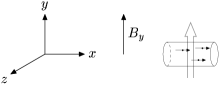
Figure 1: A $B$-field component along the $y$-axis causes a Larmor precession of an atomic spin which is initially polarized along the $x$-axis. The resulting $z$ component of the spin is probed by the Faraday polarization rotation of a linearly polarized laser beam which propagates along the $y$-axis.

A number of papers have dealt with the interaction of atomic samples with an optical field, Kuzmich et al. (1998); Takahashi et al. (1999); Kuzmich et al. (1999); Duan et al. (2000); Julsgaard et al. (2001); Mølmer and Madsen (2004); Madsen and Mølmer (2004). A particularly convenient interaction occurs when the two atomic states interact with a linearly polarized non-resonant probe field. A linearly polarized field can be expanded on two circular components, and if they interact differently with the two internal atomic states, they experience different phase shifts depending on the atomic populations, which in turn translates into a (Faraday) rotation of the polarization of the field. For use of the effective spin-$1/2$ picture to the description of angular momenta larger than $1/2$, see for example Sherson et al. (2006). We are interested in the case of a continuous beam of light interacting with the atoms, and this is effectively obtained by discretizing the field into a sequence of square pulse segments of light, see Mølmer and Madsen (2004). Since the light beam is linearly polarized along $x$, the Stokes operator for a short segment of the beam with $N_{\mathrm{ph}}$ photons has an x-component which behaves classically, $\langle S_{x}\rangle=\frac{\hbar N_{\mathrm{ph}}}{2}$, and the two remaining components fulfill the commutator relation of angular momentum operators. Accordingly, for the scaled effective variables $x_{\mathrm{ph}}=\frac{S_{y}}{\sqrt{\hbar\langle S_{x}\rangle}},p_{\mathrm{ph}}=\frac{S_{z}}{\sqrt{\hbar\langle S_{x}\rangle}}$, we have $[x_{\text{ph}},p_{\text{ph}}]=i$ and the initial coherent state of the field is a minimum uncertainty Gaussian state in these variables. When a single light segment is sent through the atomic sample, the polarization rotation is quantified by the difference between the intensities of linear polarization components at $45^{\circ}$ and $-45^{\circ}$ angles with respect to the incident polarization, i.e., by the $S_{y}$ $(x_{\mathrm{ph}})$ quantum variable. The field is not in an eigenstate of this quantity, and the measurement outcome is stochastic with a mean value governed by the mean rotation, i.e., the mean atomic population difference, and a variance given by a shot noise contribution from the photon number distribution, and by the variance of the atomic populations. In turn, the detection of the light signal causes a back-action on the quantum state of the atoms, which, depending on the total number of photons detected, shifts the mean atomic populations and reduces their widths.

As shown in Ref.Madsen and Mølmer (2004) and references therein, the polarization rotation described above is described by a simple effective Hamiltonian, and in the Heisenberg picture the atomic variables and the variables describing a single segment of the light beam of duration $\tau$ evolve as

$$x_{\text{at}} \mapsto x_{\text{at}}+\kappa\sqrt{\tau}p_{\text{ph}}, p_{\text{at}}\mapsto p_{\text{at}}$$ (2)

$$x_{\text{ph}} \mapsto\kappa\sqrt{\tau}p_{\text{at}}+x_{\text{ph}}, p_{\text{ph}}\mapsto p_{\text{ph}}$$ (3)

where the atom-light coupling strength $\kappa=\frac{d^{2}\omega}{\Delta Ac\epsilon_{0}}\sqrt{N_{\mathrm{at}}N_{\mathrm{ph}}/\tau}$ is a function of atomic parameters ($d$ is the atomic dipole moment, $\omega$ is the photon frequency, $\Delta$ is the detuning of the light from atomic resonance, and $A$ is the area of the the light field) and, notably, the total number of atoms $N_{\mathrm{at}}$ and the photon flux $\Phi=N_{\mathrm{ph}}/\tau$ in the pulse segment. Our theory is to a large extent analytical, but in order to present some of the results in graphs, we shall adopt realistic values, summarized in Table 1, for a possible experiment with cesium atoms.

Table 1: Values of physical quantities used in the numerical examples of this paper.

Physical quantity	Value
Initial uncertainty	$\Delta B_{0}={\text{\unboldmath$\mathrm{1}$}}\,\text{\unboldmath$\mathrm{pT}$}$
Total number of atoms	$N_{\mathrm{at}}=2\times 10^{12}$
Photon flux	$\Phi={\text{\unboldmath$\mathrm{5{}\times{}10^{14}}$}}\,\text{\unboldmath$\mathrm{s^{-1}}$}$
Intersection area	$A={\text{\unboldmath$\mathrm{2}$}}\,\text{\unboldmath$\mathrm{mm^{2}}$}$
Wavelength	$\lambda={\text{\unboldmath$\mathrm{852}$}}\,\text{\unboldmath$\mathrm{nm}$}$
Detuning	$\frac{\Delta}{2\pi}={\text{\unboldmath$\mathrm{10}$}}\,\text{\unboldmath$\mathrm{GHz}$}$
Atomic dipole moment	$d={\text{\unboldmath$\mathrm{2{.}61{}\times{}10^{-29}}$}}\,\text{\unboldmath$\mathrm{Cm}$}$
Coupling between atoms and $B$-field	$\mu={\text{\unboldmath$\mathrm{8{.}79{}\times{}10^{4}}$}}\,\text{\unboldmath$\mathrm{s^{-1}}$}$
Coupling between atoms and photons	$\kappa^{2}={\text{\unboldmath$\mathrm{1{.}83{}\times{}10^{6}}$}}\,\text{\unboldmath$\mathrm{s^{-1}}$}$

II.2 Gaussian state formalism

In this section, we shall assume a magnetic field $B(t)$ with an explicitly given time dependence. This analysis will be needed, when we proceed to simulate how an unknown field is estimated, since it is the actual realization of the field, that drives the atomic dynamics. The current section thus accounts for the “information available to the theorist”, whereas the proceeding section will deal with the “information available to the experimentalist” having only access to the optical detection record.

We place a spin-polarized atomic gas in the $B$-field, and probe it continuously by the polarized light beam. The Gaussian probability distribution (Wigner function) of the atomic variables and of the light pulse prior to interaction, evolves into a new Gaussian state, and the detection of the polarization rotation, which is a measurement of the field observable $x_{\text{ph}}$ leads to an update of the atomic state, but it retains the Gaussian form Eisert and Plenio (2003). We can hence describe the atomic state by the mean values and by the covariance matrix which fully characterize a Gaussian state, and we shall now summarize the dynamics of the atoms+fields with an effective formalism that describes the time evolution of the mean values and the covariances of the atomic state due to interaction and measurements.

We first define a vector of variables (operators) $\mathbf{y}=(x_{\text{at}},p_{\text{at}},x_{\text{ph}},p_{\text{ph}})^{T}$, with the corresponding vector of mean values $\mathbf{m}=\langle\mathbf{y}\rangle$ and with the covariance matrix $\boldsymbol{\gamma}$ where $\gamma_{ij}=2\text{Re}\langle(y_{i}-\langle y_{i}\rangle)(y_{j}-\langle y_{j}\rangle)\rangle$. Our Gaussian state description of the spin polarized sample and the linearly polarized light translates into the specification of the initial values,

$$\mathbf{m} =0$$ (4)

$$\boldsymbol{\gamma} =\mathbbm{1}_{4\times 4}.$$ (5)

and the update formula due to interactions during a time interval $\tau$

$$\mathbf{m} \to\mathbf{Sm}+\mathbf{v}$$ (6)

$$\boldsymbol{\gamma} \to\mathbf{S}\boldsymbol{\gamma}\mathbf{S}^{T}$$ (7)

where

$$\mathbf{S}=\begin{pmatrix}1&0&0&\kappa\sqrt{\tau}\\ 0&1&0&0\\ 0&\kappa\sqrt{\tau}&1&0\\ 0&0&0&1\end{pmatrix}$$ (8)

and

$$\mathbf{v}=(0,-\mu\tau B(t),0,0)^{T}.$$ (9)

Let us write

$$\boldsymbol{\gamma} =\begin{pmatrix}\mathbf{A}_{\gamma}&\mathbf{C}_{\gamma}\\ \mathbf{C}_{\gamma}^{T}&\mathbf{B}_{\gamma}\end{pmatrix}$$ (10)

$$\mathbf{m} =(\mathbf{m}_{A},\mathbf{m}_{B})$$ (11)

with $\mathbf{A}_{\gamma}$ the covariance matrix for the atomic variables, $\mathbf{y}_{1}=(x_{\text{at}},p_{\text{at}})^{T}$, $\mathbf{B}_{\gamma}$ the covariance matrix for the field variables, $\mathbf{y}_{2}=(x_{\text{ph}},p_{\text{ph}})^{T}$, and $\mathbf{C}_{\gamma}$ the correlation matrix between $\mathbf{y}_{1}$ and $\mathbf{y}_{2}^{T}$. When a measurement of the variable $x_{\text{ph}}$ is performed, the outcome takes on a random value, given by the Gaussian probability distribution. For a short segment of light, the mean value of $x_{\textrm{ph}}$ is $m_{3}=\kappa\sqrt{\tau}m_{2}$, and the variance is one half (the incident field variance is only infinitesimally modified by the atoms). The measurement of a value $x_{\text{meas}}$ for $x_{\text{ph}}$ collapses the field state and transforms the atomic component according to

$$\mathbf{A}_{\gamma} \to\mathbf{A}_{\gamma}-\mathbf{C}_{\gamma}(\pi\mathbf{B}_{\gamma}\pi)^{-}\mathbf{C}_{\gamma}^{T}$$ (12)

$$\mathbf{m}_{A} \to\mathbf{m}_{A}+\mathbf{C}_{\gamma}(\pi\mathbf{B}_{\gamma}\pi)^{-}((x_{\text{meas}}-m_{3}),0)^{T}$$ (13)

$$\mathbf{B}_{\gamma} \to\mathbbm{1}_{2\times 2}$$ (14)

$$\mathbf{C}_{\gamma} \to 0$$ (15)

$$\mathbf{m}_{B} \to 0$$ (16)

where $\pi=\operatorname{diag}(1,0)$ and $(\dots)^{-}$ denotes the Moore-Penrose pseudoinverse. To the lowest, relevant order, $(\pi\mathbf{B}_{\gamma}\pi)^{-}=\textrm{diag}(1,0)$. Equations (14), (15), and (16) “refresh” the atom and field variables corresponding to the subsequent light segment which has no correlations with the atoms prior to interaction. Note that the quantity $(x_{\text{meas}}-m_{3})$ is a random variable with vanishing mean and variance $1/2$, and since $\mathbf{C}_{\gamma}$ scales with $\sqrt{\tau}$, the measurement induced, random displacement of the mean values (13) can also be expressed in terms of a Wiener increment with zero mean and variance $\tau$, cf. Geremia et al. (2003); Stockton et al. (2004).

Before proceeding to the interaction between the atoms and an unknown magnetic field, we note that the dynamics in (2) is of quantum non demolition type (QND), i.e., it permits a detection of the atomic variable $p_{\text{at}}$ without changing this observable. Such a detection (carried out when the field variable $x_{\text{ph}}$ is read out after the atom-light interaction), in effect leads to squeezing of the $p_{\text{at}}$ component of the atomic spin around a random value, which is selected by the random outcome of the measurement process and by the deterministic Larmor rotation. Of course a single, infinitesimal time step as in (2,3) leads only to an infinitesimal squeezing, but as the evolution proceeds continuously in time it leads to a monotonic reduction of the variance of the atomic spin component. If atomic spontaneous decay is taken into account, the squeezing has an optimum and further interaction with the optical probe leads to incoherent depopulation among the atomic states. We are indeed able to describe also such processes in the Gaussian state formalism Mølmer and Madsen (2004); Madsen and Mølmer (2004), but since the importance of spontaneous processes is very system specific, and it can be reduced by going to sufficiently large detunings, we shall ignore spontaneous decay in the following.

III Estimation of an unknown time dependent $B$-field

The $B$-field causes the Larmor precession (2). By probing the value of $p_{\text{at}}$, we acquire information about the magnetic field if its value is not already known. In Mølmer and Madsen (2004); Petersen et al. (2005), we found that a constant magnetic field is effectively probed with a time dependent variance on the estimate given by

$$\Delta B(t)^{2}=\frac{\Delta B_{0}^{2}(1+\kappa^{2}t)}{1+\kappa^{2}t+\frac{2}{3}\kappa^{2}\mu^{2}(\Delta B_{0})^{2}t^{3}+\frac{1}{6}\kappa^{4}\mu^{2}(\Delta B_{0})^{2}t^{4}}$$ (17)

with $\Delta B_{0}^{2}$ representing our prior knowledge of the field. In the limit of $\kappa^{2}t\gg 1$, we have $\Delta B(t)^{2}\simeq 6/(\kappa^{2}\mu^{2}t^{3})$ which is independent of the prior knowledge and which reflects a more rapid reduction with time of the variance than expected from a conventional statistical argument. This is due to the atomic squeezing, as it progressively makes the system more and more sensitive to the magnetic field perturbation.

In the following, we shall generalize the analysis to the case of time dependent $B$-fields. A convenient model for a random field is a damped diffusion (Ornstein-Uhlenbeck) process, governed by the stochastic differential equation

$$dB(t)=-\gamma_{b}B(t)dt+\sqrt{\sigma_{b}}dW_{b}$$ (18)

where the Wiener increment $dW_{b}$ has a Gaussian distribution with mean zero and variance $dt$. Our task is to expose atoms to a realization of this process and to use the polarization measurements to construct an estimate for the actual current value of the field.

The Ornstein-Uhlenbeck process can be simulated on a computer, but we can also make statistical predictions, e.g., the steady state mean vanishes and the variance is

$$\textrm{Var}_{\textrm{st}}(B)=\frac{\sigma_{b}}{2\gamma_{b}},$$ (19)

and if the value of the field is estimated at time $t_{L}$ in the laboratory to be $\textrm{B}_{t_{L}}$ with a variance $V_{t_{L}}$ on the estimate, our best estimate for the value at a future time $t>t_{L}$ takes the value $\textrm{B}_{t}\exp(-\gamma_{b}(t-t_{L}))$ with a variance

$$V_{t}=V_{t_{L}}e^{-2\gamma_{b}(t-t_{L})}+\frac{\sigma_{b}}{2\gamma_{b}}(1-e^{-2\gamma_{b}(t-t_{L})}).$$ (20)

The Ornstein-Uhlenbeck process can be very slow, in which case the field retains its random value almost constantly over long times, and we expect to recover the results in Mølmer and Madsen (2004) for estimation of a constant field, because the accumulated photo detection record over time carries information about the time dependent field, which is known to differ not very much. If the Ornstein-Uhlenbeck process is very fast, the accumulated photo detection record until the present time $t$ gives only little information about the present value. Note that by scaling $\gamma_{b}$ and $\sigma_{b}$ by the same factor, the variance (19) is unchanged, but the process changes from slow to rapid fluctuations.

Our theoretical description of the estimation process deals with a joint Gaussian distribution for the quantum variables and the classical magnetic field. As in Mølmer and Madsen (2004) we formally treat the B-field as the first component in our vector of five Gaussian variables $\mathbf{\widetilde{y}}=(B,x_{\text{at}},p_{\text{at}},x_{\text{ph}},p_{\text{ph}})$, where the tilde is used to distinguish these variables from those in the previous section. The Gaussian state is characterized by its mean value vector $\mathbf{\widetilde{m}}=\langle\widetilde{y}\rangle$ and its covariance matrix $\boldsymbol{\widetilde{\gamma}}$ where $\widetilde{\gamma}_{ij}=2\text{Re}\langle(\widetilde{y}_{i}-\langle\widetilde{y}_{i}\rangle)(\widetilde{y}_{j}-\langle\widetilde{y}_{j}\rangle)\rangle$.

Note that although, e.g., $x_{\text{at}}$ is the same operator in this and the previous section, its Gaussian state mean value and variance are not the same, because the Gaussian state is the probability distribution assigned by the observer given his or her acquired knowledge about the system. In the previous section we determined this probability distribution conditioned on full knowledge of the time dependent $B$-field and the photo detection record, whereas in the current section, only “the experimentalist’s” knowledge of the detection record is assumed.

By propagating the update formulas for $\mathbf{\widetilde{m}}$ and $\boldsymbol{\widetilde{\gamma}}$ due to the Larmor rotation, the atom-light interaction, the random outcomes of the probing process, and the Ornstein-Uhlenbeck process, we obtain at any time a mean value $\widetilde{m}_{1}$ and a variance $\widetilde{\gamma}_{11}/2$ for the $B$-field.

The initial values are

$$\mathbf{\widetilde{m}} =0$$ (21)

$$\boldsymbol{\gamma}_{0} =\operatorname{diag}(2\operatorname{Var}(B_{0}),1,1,1,1).$$ (22)

Due to the interaction between the $B$-field and the atoms and between the atoms and the photons we have

$$\mathbf{\widetilde{m}} \to\mathbf{S}_{1}\mathbf{\widetilde{m}}$$ (23)

$$\boldsymbol{\widetilde{\gamma}} \to\mathbf{S}_{1}\boldsymbol{\widetilde{\gamma}}\mathbf{S}_{1}^{T}$$ (24)

where

$$\mathbf{S}_{1}=\begin{pmatrix}1&0&0&0&0\\ 0&1&0&0&\kappa\sqrt{\tau}\\ -\mu\tau&0&1&0&0\\ 0&0&\kappa\sqrt{\tau}&1&0\\ 0&0&0&0&1\end{pmatrix}$$ (25)

In this section the $B$ field is one of the variables, and hence the equation (23) is linear unlike the affine transformation (6). Due to the Ornstein-Uhlenbeck process we have

$$\widetilde{m}_{1} \to\widetilde{m}_{1}(1-\gamma_{b}\tau)$$ (26)

$$\boldsymbol{\widetilde{\gamma}} \to\mathbf{S}_{2}\boldsymbol{\widetilde{\gamma}}\mathbf{S}_{2}+\mathbf{L}$$ (27)

where $\mathbf{S}_{2}=\operatorname{diag}(1-\gamma_{b}\tau,0,0,0,0)$ and $\mathbf{L}=\operatorname{diag}(\sigma_{b}\tau,0,0,0,0)$.

To handle the measurement on $\widetilde{x}_{\text{ph}}$ we write the covariance matrix and mean value vector as

$$\boldsymbol{\widetilde{\gamma}} =\begin{pmatrix}\mathbf{\widetilde{A}}_{\gamma}&\mathbf{\widetilde{C}}_{\gamma}\\ \mathbf{\widetilde{C}}_{\gamma}^{T}&\mathbf{\widetilde{B}}_{\gamma}\end{pmatrix}$$ (28)

$$\mathbf{m} =(\mathbf{m}_{A},\mathbf{m}_{B})$$ (29)

with $\mathbf{\widetilde{A}}_{\gamma}$ the covariance matrix for the $B$-field and atoms, $\mathbf{\widetilde{y}}_{1}=(B,\widetilde{x}_{\text{at}},\widetilde{p}_{\text{at}})^{T}$, $\mathbf{\widetilde{B}}_{\gamma}$ the covariance matrix for the photons, $\mathbf{\widetilde{y}}_{2}=(\widetilde{x}_{\text{ph}},\widetilde{p}_{\text{ph}})^{T}$, and $\mathbf{\widetilde{C}}_{\gamma}$ the correlation matrix for $\mathbf{\widetilde{y}}_{1}$ and $\mathbf{\widetilde{y}}_{2}^{T}$. The measurement of $\widetilde{x}_{\text{ph}}$ then transforms these matrices according to

$$\mathbf{\widetilde{A}}_{\gamma} \to\mathbf{\widetilde{A}}_{\gamma}-\mathbf{\widetilde{C}}_{\gamma}(\pi\mathbf{\widetilde{B}}_{\gamma}\pi)^{-}\mathbf{\widetilde{C}}_{\gamma}^{T}$$ (30)

$$\mathbf{\widetilde{B}}_{\gamma} \to\mathbbm{1}_{2\times 2}$$ (31)

$$\mathbf{\widetilde{C}}_{\gamma} \to 0$$ (32)

$$\mathbf{\widetilde{m}}_{A} \to\mathbf{\widetilde{m}}_{A}+\mathbf{\widetilde{C}}_{\gamma}(\pi\mathbf{\widetilde{B}}_{\gamma}\pi)^{-}(x_{\text{meas}}-\widetilde{m}_{4},0)^{T}$$ (33)

$$\mathbf{\widetilde{m}}_{B} \to 0$$ (34)

These equations fully describe the conditioned and the deterministic evolution of the multi-variable Gaussian distribution, and in particular we get access to the estimator for the $B$-field in the form of its mean and the corresponding covariance matrix element. The input to the estimation protocol is the constant parameters of the problem and the outcome of the photo detection, which will drive the mean values, and hence the estimator, to a non-trivial result, cf. Eq. (33). We note that whereas the estimator depends on the actual measurement outcome, the covariance matrix evolves in an entirely deterministic manner, and we can hence theoretically predict the magnitude of the error as it was also done in Stockton et al. (2004).

We wish to simulate the protocol with a given realization of the noisy field, and to this end we have to combine the theories of this and the previous section. In such a simulation it is the actual field $B(t)$ that acts on the atoms and hence leads to the probability distribution for the photo detection record, and the measured quantum field variable $x_{\text{ph}}$ has the mean value $m_{3}=\kappa\sqrt{\tau}m_{2}$, given by the expressions of the previous section. Hence the measurement outcome can be written $\kappa\sqrt{\tau}m_{2}+\chi$ where $\chi$ is uncorrelated with its value at previous detection times, and it has vanishing mean and a variance of $1/2$. We are thus effectively communicating the value of the simulated $B$-field through the use of the “theorist’s” estimator of the atomic state in the simulation of measurement outcomes. Assuming a random measurement outcome with the statistics described, we update the mean value vector and covariance matrix of the previous subsection, and we use the same simulated measurement outcome in the update formula (33). The simulated measurement outcome may deviate from the value $\widetilde{m}_{4}$ currently expected by the “experimentalist” both because of the noisy contribution and because the mean is given by its true value and not by his or her estimate. The latter is responsible for driving the $B$-field estimate towards the actual realization in our numerical simulations.

IV Results

We now have a complete theory which, given the detection record, provides the estimator for the time dependent $B$-field and its variance. In practice, the experiment should be run, and the analysis should be applied on the full detection record, either simultaneously with the experiment or afterwards. Some calculation is necessary since the $B$-field estimator at any time involves knowledge of the full vector of mean values and the covariance matrix. The covariance matrix, and in particular the variance of the $B$-field estimate evolves deterministically with time. We can in fact solve the equations for the covariance matrix analytically, and in the long time limit we find the steady state variance on our $B$-field estimate:

$$\begin{split}\operatorname{Var}(B)&=\frac{1}{4\kappa^{2}\mu^{2}}\Bigl{(}\sqrt{\gamma_{b}^{2}+2\mu\sqrt{\sigma_{b}}\kappa}-\gamma_{b}\Bigr{)}^{2}\\ &\mathrel{\phantom{=}}\times\sqrt{\gamma_{b}^{2}+2\mu\sqrt{\sigma_{b}}\kappa}.\end{split}$$ (35)

When the Ornstein-Uhlenbeck process is slow, early detection events and estimates provide already an estimate for future values of the field, cf. (20), which is further refined by the continued measurement record. As also shown by (20), if the rate $\gamma_{b}$ is high, the estimates quickly loose their significance, and only probing for a short time before $t$ is useful in the estimate of of $B(t)$. In Fig. 2 we show how the variance of the $B$-field estimate starts with the prior steady state value (19) before any probing takes place, and evolves to the steady state value given by (35). In the figure we assume the same steady state value for the $B$-field variance $\sigma_{b}/2\gamma_{b}$ in all curves, but with different values of the fluctuation rate constant $\gamma_{b}$. For comparison we show also in the figure the analytical result (17) for a constant, unknown field with the same prior uncertainty. This curve converges to zero, but it is clearly seen to follow the curves with finite $\gamma_{b}$ on short time scales (determined by $\gamma_{b}$).

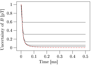
Figure 2: Uncertainty of the $B$-field as a function of time. We have used the numerical values of Table 1. The dashed/red line is the analytical result for a constant $B$-field. The full/black lines represents fluctuating fields with the same steady state uncertainty $\sqrt{\sigma_{b}/2\gamma_{b}}=1\textrm{pT}$, but with decreasing rates. From above, $\gamma_{b}={\text{\unboldmath$\mathrm{10^{5}}$}}\,\text{\unboldmath$\mathrm{s^{-1}}$},{\text{\unboldmath$\mathrm{10^{4}}$}}\,\text{\unboldmath$\mathrm{s^{-1}}$},{\text{\unboldmath$\mathrm{10^{3}}$}}\,\text{\unboldmath$\mathrm{s^{-1}}$},{\text{\unboldmath$\mathrm{10^{2}}$}}\,\text{\unboldmath$\mathrm{s^{-1}}$},{\text{\unboldmath$\mathrm{10^{1}}$}}\,\text{\unboldmath$\mathrm{s^{-1}}$}$. For small values of $\gamma_{B}$ the full/black curves approach the constant $B$-field result as expected.

In Fig. 3 we show the result of the application of a given realization of the Ornstein-Uhlenbeck process. The figure shows the actual process as a full line and the estimator as a dashed line for a typical time window. We observe that the estimator tracks the gross structure of the dependence very well, but smaller transients are not reproduced. Taking a second look at the figure, we also observe that the estimate is systematically lagging behind the true realization of the field. This is not surprising, as the estimate makes explicit use of all past measurements to predict the current value. In particular, if no measurement results are provided, the estimate for the value is simply obtained from past values according to Eq. (18). This should, however, prompt attempts to make an even better estimate for the field using not only the detection record until the instant of interest, but also the later detection events. We recall that we are actually probing the atomic spin state, and the Larmor precession due to the $B$-field may well be detected also after it took place.

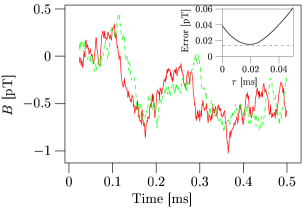
Figure 3: Time dependent value of the actual, simulated $B$-field (full/red line) and the estimate based on a simulated detection record (dashed/green line). The atomic parameters are given in Table 1, and the $B$-field is characterized by $\gamma_{b}={\text{\unboldmath$\mathrm{10^{3}}$}}\,\text{\unboldmath$\mathrm{s^{-1}}$}$ and $\sigma_{b}={\text{\unboldmath$\mathrm{2{}\times{}10^{3}}$}}\,\text{\unboldmath$\mathrm{pT^{2}/s}$}$. The inset shows the error of the estimate (36) as a function of a variable translation of the two curves with respect to each other, and the horizontal dashed line in the inset shows the error obtained from a weighted average of delayed estimates, see text and Eq. (37).

To justify this increased effort, we have made a very simple transformation of the data, consisting in a temporal displacement of the two curves in Fig. 3, so that we compare the current estimator $\widetilde{m}_{1}(t)$, obtained by our theory with earlier values of the field $B(t-T)$. The inset of Fig. 3 shows the numerically calculated error of the estimate, averaged over a long detection record, plotted as a function of the delay $T$,

$$\mathrm{Error}^{2}(T)=\frac{1}{t_{0}}\int_{T}^{t_{0}+T}(\widetilde{m}_{1}(t)-B(t-T))^{2}dt,$$ (36)

and we indeed see, that for a range of values for $T$ the error is smaller than for $T=0$, i.e., we obtain a better estimate if we assign our estimate to the value of the $B$-field a little earlier.

A slightly more elaborate procedure to improve the estimate obtained from the above procedure is obtained by assuming not just a simple delay but a temporal convolution of the estimators, $B_{opt}^{est}(t)=\int_{-\infty}^{\infty}a(t-t^{\prime})\widetilde{m}_{1}(t^{\prime})dt^{\prime}$. Numerically, we have identified the optimum delay distribution by minimizing the (squared) error

$$\frac{1}{t_{0}}\int_{T}^{t_{0}+T}\Bigl{(}\sum_{i}a_{i}\widetilde{m}_{1}(t-idt)-B(t)\Bigr{)}^{2}dt,$$ (37)

which turns out to be a linear algebra problem for the coefficients $a_{i}$. Running a series of simulations, we find the temporal variation of the delay distribution plotted in Fig. 4, peaking, as expected, around the optimum delay, found in Fig. 3. The error obtained this way is smaller than by use of any fixed delay, as indicated by the horizontal dashed line in the inset in Fig. 3.

Figure 4: Time dependence of optimal weight factors $a_{i}$ in Eq. (37), favoring contributions with a finite delay around 0.02 ms as suggested by the insert in Fig. 3.The atomic parameters are given in Table 1, and the $B$-field is characterized by $\gamma_{b}={\text{\unboldmath$\mathrm{10^{3}}$}}\,\text{\unboldmath$\mathrm{s^{-1}}$}$ and $\sigma_{b}={\text{\unboldmath$\mathrm{2{}\times{}10^{3}}$}}\,\text{\unboldmath$\mathrm{pT^{2}/s}$}$.

IV.1 “Gaussian theory of hindsight”

Both the fixed delay and the weighted average of delays bring promises for improved sensitivity of magnetometers, if one can wait for the estimate until (a short time) after the action of the field. Both procedures, however, suffer from their ad hoc character, and in particular from the fact that the optimum delay or delay distribution are not theoretically available, unless one accepts to use simulations as the present ones a guideline. We shall now present the correct theory, which gives the optimum estimate and a tight bound on the error without any ad hoc procedures.

The current estimate of the $B$-field is given by a Gaussian probability distribution, and so is the estimate of the value at all points in the past, and as measurements on the atoms proceed, we may keep improving also our past estimate. We hence treat not only the current value but also past values of the B-field as Gaussian variables together with the atom and field variables. To update the estimate at an instant $T$ in the past, we need to keep track of the entire interval from $t-T$ to the present time $t$, and we extend our Gaussian state formalism by replacing the argument $\widetilde{y}_{1}$ by a whole vector of values, representing the unknown $B$-field at discrete times spanning an interval from $t-T$ until $t$. Since we are dealing with the values in the past, they are not evolving due to the Ornstein-Uhlenbeck process, but inherit their randomly value as time proceeds and the elements in the vector of mean values and the covariance matrix are simply “pushed towards the past”. Only the current value of $B(t)$ is given by the stochastic process. The atomic system is correlated with both the current and the previous values of the field as witnessed by non-vanishing elements in the extended covariance matrix, and hence the updating due to measurements on the atoms also influence the variance of the B-field estimate in the past, c.f. the appropriate generalization of Eq. (33). Now, there is nothing ad hoc about the procedure. At any time, we have an estimator for the value of the field over a finite interval looking backwards in time, and we have the variance of these values, which is a decreasing function of the time difference, approaching a constant, for values so long time ago, that their action on the atoms is no longer discernible, and hence no further updating takes place due to Eq. (33).

Fig. 5 shows a comparison of the actual, simulated field with our Gaussian estimator, available 0.1 ms after the action of the $B$-field on the atoms. Rapid transients are not reproduced, but in comparison with Fig. 3, we have clearly removed the lag and improved the overall agreement between the estimator and the actual value of the time dependent field.

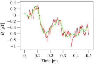
Figure 5: Time dependent value of the actual, simulated $B$-field (full/red line) and the estimate based on a simulated detection record available until 0.1 ms after the action of the field (dashed/green line). The atomic parameters are given in Table 1, and the $B$-field is characterized by $\gamma_{b}={\text{\unboldmath$\mathrm{10^{3}}$}}\,\text{\unboldmath$\mathrm{s^{-1}}$}$ and $\sigma_{b}={\text{\unboldmath$\mathrm{2{}\times{}10^{3}}$}}\,\text{\unboldmath$\mathrm{pT^{2}/s}$}$.

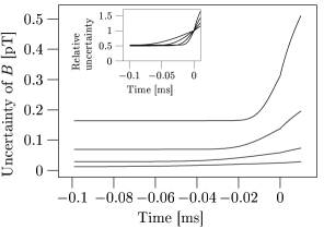
Figure 6: Time dependence of the variance of our estimate of the time dependent field $B(t)$-field around the current time $t_{L}$ in the laboratory. The curves represent fluctuating fields with the same steady state uncertainty $\sqrt{\sigma_{b}/2\gamma_{b}}=1\textrm{pT}$, but with decreasing rates. From above, $\gamma_{b}={\text{\unboldmath$\mathrm{10^{4}}$}}\,\text{\unboldmath$\mathrm{s^{-1}}$},{\text{\unboldmath$\mathrm{10^{3}}$}}\,\text{\unboldmath$\mathrm{s^{-1}}$},{\text{\unboldmath$\mathrm{10^{2}}$}}\,\text{\unboldmath$\mathrm{s^{-1}}$},{\text{\unboldmath$\mathrm{10^{1}}$}}\,\text{\unboldmath$\mathrm{s^{-1}}$}$. The atomic parameters are given in Table 1. For later times $t>t_{L}$, we have to guess the value from the properties of the Ornstein-Uhlenbeck process (20), at the current time we have the value (35), and for earlier times we get the improvement given by the solution of the extended Gaussian state updating. The inset shows the uncertainty relative to its value at $t=t_{L}$; improved by an approximate factor of 2, when we estimate the past values of the field.

Fig. 6 reports the variance of the estimate of the $B(t)$-field plotted at a given time $t_{L}$ in the laboratory after a long measurement time, so transients in the atomic dynamics have died out. Results are shown for different values of $\gamma_{b}$ but a constant ratio between $\gamma_{b}$ and $\sigma_{b}$. The estimate for $B(t=t_{L})$ at the laboratory time is based on measurements that have registered the action of the field at all previous times and takes the value given by (35). For future times $t>t_{L}$, we have to use the current estimate and extend it by our knowledge of the Ornstein-Uhlenbeck process, i.e. by inserting $V_{t_{L}}$ in Eq. (20). The curves show that it is easier to guess the present value than future ones, and that future values are particularly hard to guess for a rapidly fluctuating process. Finally, the curves also explore the range of $t<t_{L}$, where we estimate past values of the field, and we observe the value of hindsight. For small $\gamma_{b}$, the uncertainty is small, but we see in the inset of the figure, where the variance is plotted relative to its value at $t=t_{L}$, that quite independently of the time constant of the fluctuations, if we can only wait long enough, we find an improvement by a factor of approximately 2 on the uncertainty compared to the equal time estimate. This improvement is a function of the physical coupling parameters, and the present study suggests a careful analysis of the optimum probing strategy, including the possibility of time dependent probing field strengths and detunings and taking into account also atomic decay processes.

V Discussion

We have presented a formalism, that provides the correct estimate of a time dependent $B$ field which is known to fluctuate randomly according to an Ornstein-Uhlenbeck process. The estimate exhausts the measurement data and makes the tightest possible conclusions from the photo detection record. It is “correct” in the sense that any better estimate necessarily requires further information, which could either be in the form of prior information about the field or the results of further measurements on the system. Our ability at time $t$ to estimate $B(t)$ connects in a natural manner with previous results for the estimation of static fields, and it is comparable with the results of the analysis of time dependent fields in Stockton et al. (2004). Simulations show that this theory actually provides a better estimate of the value in the recent past (or, instrumentally, if you need to estimate the field at time $t$, you should use the formally obtained estimate at time $t+T$ for some suitable $T$). Our formalism naturally generalizes to describe also a scenario, where previous estimates are updated by current measurements, and this provides an essential improvement for magnetometers as documented in the paper.

We have not made a complete survey of the optimal performance as a function of all physical parameters. At this stage, it seems futile to vary all parameters without inclusion, in particular, of atomic decay, which will either restrict the magnetometers to finite time analyses or which will have to be compensated by a continuous optical re-pumping of the atoms. As pointed out in Stockton et al. (2004), the field estimation can be made robust to imprecise information about some of the physical parameters, in particular the number of atoms which enters the atom-light interaction strength. Instead of just calculating the field, one can apply, in a feed back set-up, a compensating field which should freeze the Larmor precession, independently of the number of atoms, and the field estimate is now given by the value of this compensating field. It is possible to include a time dependent feed back field in our equations, and hence to simulate the performance of any feed back strategy and its robustness against fluctuations in physical parameters. Another important extension of the theory deals with the assumption of the Ornstein-Uhlenbeck process with given parameters. The parameters enter explicitly in our estimation procedure, and if these parameters are not known, or if they are functions of time, e.g., as in the case of cardiography on a beating heart, more refined theory will bee needed. At this point, we recall, that the Ornstein-Uhlenbeck model represents our prior knowledge about the field fluctuations. A conservative high estimate on the noise fluctuations will hence give a similar conservative estimate on the field, which might be improved if better limits were known. A theoretical investigation of this problem could for example simulate the estimation of a noisy field, assuming a different value of the parameters than applied in the synthesis of the field, and investigate numerically the difference between the variance on the estimate obtained from the theory and the actual statistical agreement between the estimate and the field.