Classical simulators of quantum computers and no-go theorems
Abstract
It is discussed, why classical simulators of quantum computers escape from some no-go claims like Kochen-Specker, Bell, or recent Conway-Kochen “Free Will” theorems.
1 Introduction
A term “quantum computer” was introduced just twenty five years ago, 7 May 1981, by Feynman in his lecture “Simulating Physics with Computers” [1] at the conference on Physics and Computation.
In this lecture Feynman said [1, p 471]
[…] “Might I say immediately, so that you know where I really intend to go, that we always have had (secret, secret, close the doors!) we always have had a great deal of difficulty in understanding the world view that quantum mechanics represents. At least I do, because I’m an old enough man that haven’t got to the point that this stuff is obvious to me. Okay, I still get nervous with it. And therefore, some of the younger students … you know how it always is, every new idea, it takes a generation or two until it becomes obvious that there’s no real problem. It has not yet become obvious to me that there’s no real problem. I cannot define the real problem, therefore I suspect there’s no real problem, but I’m note sure there’s no real problem. So that’s why I like to investigate things. Can I learn anything from asking this question about computers—about this may or mat not be mystery as to what the world view of quantum mechanics is?” […]
He also explained, why “asking questions about computers” may be useful [1, p 486]
[…] “So, I would like to see if there’s some other way out, and I want to emphasize, or bring the question here, because the discovery of computers and the thinking about computers has turned out to be extremely useful in many branches of human reasoning. For instance, we never really understood how lousy our understanding of language was, the theory of grammar and all that stuff, until we tried to make a computer which would be able to understand language. We tried to learn a great deal about psychology by trying to understand how computers work. There are interesting philosophical questions about reasoning, and relationship, observation, and measurement and so on, which computers have stimulated us to think about anew, with new types of thinking. And all I was doing was hoping that the computer-type of thinking would give us some new ideas, if any are really needed.” […]
Being only embarked in theory of quantum computers about 15 years ago, author often encountered an idea that results like Kochen-Specker theorem may prevent successful simulation of such quantum devices on classical computers. The doubts were dispelled later due to papers like [2, 3] and appearance of first programs-simulators of quantum computers.
In the Feynman lecture [1] as well as in later works, which provided base of modern theory of quantum computation [4, 5, 6, 7], is written only about limitations due to exponential growth of complexity, but not about principle impossibility of modeling.
Formally, any classical program-simulator is some nonlocal model of quantum computer and it let avoid limitation risen by Bell consideration [8]. On the other hand, it appears, that Kochen-Specker theorem [9, 10] is concerned with some other class of limitations.
It is interesting to apply “computer-type of thinking” by considering principles and problems of simulation of Bell experiments with two spin-half systems [8], model with spin-1 system used in Kochen-Specker theorem [9], as well as experiments with both kinds of problems, like discussed in [11].
In the Sec. 2 is considered a minimalistic model, well known from theory of quantum computations and appropriate for consideration of most (thought) experiments with quantum systems used in no-go theorems mentioned above. It is applied first in Sec. 3 to consideration of models used in Kochen-Specker theorem. Next sections are devoted to nonlocal models. In Sec. 4 is discussed Bell pair, i.e., compound system with two qubits. Model with two spin-1 systems used in Conway-Kochen “Free Will” theorem is briefly analyzed in Sec. 5. In Sec. 6 is revised the problem with relativity principle for measurement of nonlocal quantum systems.
2 Simulation of quantum computer
Minimal model with pure states may be defined as:
-
•
States: Pure state is defined as normalized vector in Hilbert space , . (More precisely, the state is element of space of rays, i.e., complex projective space111Complex projective space is space of rays in , i.e., factor space , , . If to express , it can be considered as space of normalized complex vectors (that is equivalent to real hyper-sphere ) modulo phase (circle ). ).
-
•
Composition: State of compound system is described by tensor product of Hilbert spaces .
-
•
Gate: Quantum gate is any unitary operator on Hilbert space of given quantum system .
-
•
1-Measurement (“filter”): Such measurement is described by filter and has analogue with question “Is it similar with ?” that for some state produces (answer “yes”) with probability (square of scalar product) or “nothing.”
-
•
N-Measurement (“basis”): Measurement in given complete orthogonal basis , . For given produces one between outputs with probability .
-
•
P-Measurement (“partial”): It is given set of projectors corresponding to decomposition of on direct sum of orthogonal subspaces (not necessary rays). For given produces with probability normalized output .
-
•
-Measurement (values of operators). Let is (Hermitian) operator. It is used previous P-measurement procedure with are projectors on eigenspaces of . Now output with probability is corresponding eigenvalue, i.e., .
References: Chapters 1–3 of [12] for introduction to quantum theory and Dirac bra, ket notation, [13] for von Neumann theory of quantum measurements, [14] for introduction to theory of quantum computation with pure states.
Any classical simulator of quantum computer might be considered formally as a hidden variable model of quantum system and so may be interesting for general discussions on foundations of quantum mechanics. The model discussed here is quite rough and can be simply adapted for realization on classical computer: state is described as complex array represented as real numbers, gate is a complex matrix, measurements are reproduced by standard routines with random number generator.
The simple model could not substitute any “serious” interpretation of quantum mechanics. It should be used with care, say measurements must be only performed after all quantum gates and consequent measurements are permitted only for commuting projectors But such a model is enough for most examples in given paper.
For more complicated schemes of quantum circuits, measurement and channels may be used models with mixed states [15]. Sometimes it is convenient to work with density matrix even for pure state
| (1) |
In such a case all formulas for probabilities used above should be rewritten using equation like
| (2) |
It is also possible for some cases to consider even simpler model with real spaces and spheres. Such kind of models are also illustrative, because very similar with some pure classical models used in theory of statistical images (patterns) recognition [16]. Such property let us talk about such models not only as some reduced model of quantum mechanics, but also as about more or less “natural” example of classical statistical model and use it as test of some assumptions about hidden variables.
3 Kochen-Specker theorem
3.1 Simplified abstract model
Let us first consider simulation of quantum systems, used in an abstract geometric version of Kochen-Specker model [9, 10], i.e., it is considered sphere in Euclidean space , orthogonal frames (without relation with directions in physical space), and only one-dimensional projectors associated with vectors of the frames . Let us consider applications of model discussed in Sec. 2 for three-dimensional case. It will be also used simplified version of model from Sec. 2 with simulation on real space instead of complex one, i.e., sphere in 3D space.
A state is described by triple of real numbers , , aka “color (red, green, blue)”. The measurements models here are very simple: 1-measurement declares, that for filter, described by triple the probability of “yes” answer is equal of square of scalar product .
An N-measurement (here ) in a basis (frame) with three vectors , and is also quite straightforward: for any state and frame there are probabilities
| (3) |
that the measurement produces result , or respectively.
Formally, it is a hidden variables model, because here state is described by two real parameters (say two Euler angles on sphere), but any measurement may produce only discrete outcome with two (yes/no) or three values (say 1, 2 or 3 for “branches” , or respectively).
It should be mentioned, that in such description the model is not “contextual,” because probability of each outcome in Eq. (3) depends only on given vector, but not other components of frame.
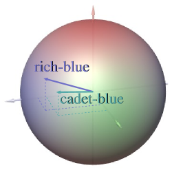
Let us use example with colors (Fig. 1). If we have some unknown color, then for 1-measurement it is possible to ask “Is it blue color?” If it really was some “rich-blue color” , then “yes” has probability (). It is possible also to use question with other sample, for example “Is it cadet-blue color?”, where “cadet-blue color” corresponds to vector . In such a case, answer “yes” has probability ().
Let us consider now the 3-measurement for frame. For “rich-blue color” it produces one of three outputs: “red,” “green,” or “blue” with probabilities 16/81, 16/81 and 49/81 respectively. It should not be mixed with three independent questions, when it is possible to get from zero to three positive answers. It is possible to calculate probabilities for zero, one, two and three answers “yes” respectively:
For example with “rich-blue” color approximate values of the probabilities are 25.4% (0), 51.5% (1), 20.7% (2), 2.4% (3), i.e., only for 51.5% cases here is one “yes”. Only if one of is unit and all other are zeros the probability of one “yes” is 100%.
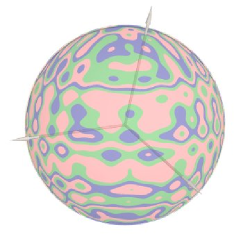
Let us consider a geometric interpretation of Kochen-Specker theorem (Fig. 2): It is impossible to have 3-coloring of sphere with property, that any three orthogonal arrows point to different colors. It is equal reformulation of Kochen-Specker theorem with three colors instead of two numbers [9, 10], it is enough to assign unit to red and green areas and zero to blue ones.
A short and understending formulation and interpretation of abstract Kochen-Specker theorem [10, §7-3]:
“ The Kochen-Specker theorem asserts that, in a Hilbert space of dimension , it is impossible to associate definite numerical values, 1 or 0, with every projection operator , in such a way that, if a set of commuting satisfies , the corresponding values, namely or , also satisfy . The thrust of this theorem is that any cryptodeterministic theory that would attribute a definite result to each quantum measurement, and still reproduce the statistical properties of quantum theory, is inevitably contextual. In the present case, if three operators, , , and , have commutators and , the result of a measurement of cannot be independent of whether is measured alone, or together with , or together with .”
Eq. (3) ensure that probability depends only on and coincides with probability for 1-measurement, and so it does not matter, if instead of frame is used some other one or is measured alone. If the model of measurement described in Sec. 2 “independent of whether is measured alone, or together with , or together with ”?
It is impossible to simulate measurements , , and in single run (here the model reproduces standard property of quantum mechanics) and so it is not possible to ask about definite results of such measurements — they are not defined in the model as well as in quantum mechanics. If to talk about different runs, then even two measurements of the same alone may produce different results.
From such a point of view the model is not contextual, it is simply statistical, but for simulation of quantum system on deterministic classical computer it is necessary to suggest some algorithm for implementation of such statistical model. For generation of three numbers with given probabilities , , it is commonly used generator of random numbers with uniform distribution . The output is defined using inequalities:
| (4) |
The method may be simply generalized for arbitrary number of outcomes with rules for .
Here problem of contextuality may appear again: if to try to model different experiments with same “hidden variable” , then appearance of the value depends on via in Eq. (4). But similar problems may appear in pure classical statistical “paradoxes,” for models with three outcomes. Well known example is “paradox” with division of a stick on three parts in classical theory of geometrical probabilities [21, 22]. We may ask here questions similar with discussed above, i.e., ‘What is hidden variable model for such division?’, ‘How does length of first part is correlated with other ones?’, or even, ‘Does it possible to suggest a model, that may “naturally” simulate this process?’ The last question about existence of a model is not unusual, in fact, it is just a reason, why such a problem is called “paradox.”
It is possible to consider simpler example of pure classical statistical “paradox,” relevant with present discussion. Let we have roulettes with red, green and blue areas (with angles , , ) for modeling an outcome with probabilities , , (Fig. 3). If appearance of green color depends only on value ? Yes, by definition! But in computer model of roulette with hidden parameter and algorithm like Eq. (4) it formally depends also on , yet it may not be found by any statistical test.

3.2 Physical model
It is more interesting to consider simulation of model, used in physical interpretation of Kochen-Specker theorem [9, 10]. Here is used presentation of momentum operators in symmetrical form [10] (system of units with )
| (5) |
Let us write eigenvectors of each operator:
| (\theparentequationx) | |||
| (\theparentequationy) | |||
| (\theparentequationz) |
where eigenvectors , correspond to eigenvalues of operator .
In Kochen-Specker theorem are used commuting operators [9, 10]
| (7) |
where . It is possible to measure all the values in one measurement of an operator [9], e.g., operator
| (8) |
The operator has eigenvalues with eigenvectors
| (9) |
It is possible to express using
| (10) |
It is convenient, that Eq. (5) in such presentation are real matrixes and coincide with generators of SO group on real subspace of full Hilbert space of spin-1 system. Eigenvectors Eq. (9) of also may be considered as elements of . So geometrical model with real 3D space and its rotations (‘-sphere’) used in Kochen-Specker theorem is justified here.
Let us consider transition to some other frame, i.e.,
| (11) |
The transition Eq. (11) is described by some orthogonal matrix , composed from elements of the frame
| (12) |
It is simple to find expression for any for new frame, e.g.
| (13) |
and analogue expressions valid for and . For particular example of frame with same vector the matrix is
| (14) |
and so (and in Eq. (5), but in Eq. (\theparentequationx) produces a phase multiplier).
It should be mentioned only, that geometrical interpretation with directions in real physical space does not look so obvious. Eigenvectors of coincide with eigenvectors for zero eigenvalues for three different operators Eq. (6), but it is hardly to consider as some directions “zero projections of momentum”. Eigenvectors for different momentum are not orthogonal and have equal scalar products and so a visual classical picture with three orthogonal axes is not quite justified.
The eigenvalue of corresponds to 2D eigenspace, i.e., after normalization it is some subspace in isomorphic to Riemann sphere, that intersects -sphere along big circle and so picture is rather complicated. The quantum mechanical description of spin-1 particle essentially differs from classical, it may not be presented as some vector in 3D space. In model with pure states from Sec. 2 it is described by complex projective space , that may be represented as nontrivial four-dimensional real manifold , but not as classical model with sphere of unit vectors in .
Let us now consider measurements of using model from Sec. 2. If there is some state , then measurement of produces , , with probabilities , , respectively. Each value of corresponds to certain combination of values , , , i.e., , , .
It is also possible to use few separate P-measurements. Scheme of all outcomes for consequent measurements , , is depicted below (Tab. 1) and it can be found, that , , . It is also possible to write probabilities of measurement of values 0 and 1 for any , e.g. , , , , , .
For any order of measurements the probabilities are the same. Using more general arguments, it is possible to say, that for commuting operators different procedures of P-measurements simply reproduce classical statistical manipulations with -algebra with three elements and measure .
It is also possible to consider some other frame with the same and other , . It corresponds to decomposition of a state using other with frame matrix Eq. (14) and eigenvectors Eq. (11) , , , i.e., with only two changed projectors and probabilities , so here again and .
So statistical model should not be treated as contextual, but modeling with deterministic computer and random number generator may essentially depend on order of operations.
The Kochen-Specker theorem disproves possibility of specific hidden variables model, that could provide more detailed deterministic description of system, than quantum mechanics itself or minimal model from Sec. 2. Even if using some analogues of Kochen-Specker model, like design with slightly nonorthogonal directions discussed in [17, 19] and criticized in [18, 20], we could produce some deterministic description, it would be quite contradictory achievement, because let us talk about things impossible in usual quantum mechanics, like simultaneous values for noncommuting operators222Yet, there are some arguments in support of the counterfactual reasoning in [10]..
4 Bell pair
4.1 Nonlocality and relativity
The problem with deterministic model is especially clear, when order of operations is not determined, e.g., due to relativity principle it may be not defined, whose measurement was first, or second, or it was all simultaneous. So statistical model may be invariant, because probabilities are not depend on order, but deterministic implementation has the problems with principle of relativity.
Model described in Sec. 2 become nonlocal, then requires possibility of instanteneous operations on whole system with few separate parts. There is standard way to show problems with such description, that was introduced first in famous Einstein-Podolsky-Rosen paper [23] and discussed further by Bell [24, 25].
The simultaneous measurement procedure may be described via set of projectors . Another method — is to use “partial” measurements, i.e., separate procedure for first or second system, described with or respectively. It is possible also to chose different bases for each system and to use other commuting sequences of measurements like , , .
Let us consider so-called Bell state of two spin systems
| (15) |
Here second expression is used in theory of quantum computation, there system with two states is called qubit with notation and for two basic states.
The singlet state Eq. (15) does not depend on change of basis
| (16) |
4.2 Description of single system (qubit)
It is convenient to consider first property of single spin system or qubit. The spin operators () are expressed via Pauli matrixes
| (17) |
It is possible also to introduce set with three pairs of orthogonal projectors
| (18) |
They corresponds to measurement of spin along axes .
Measurement along arbitrary axis is described using projectors
| (19) |
where two orthogonal projectors correspond to Eq. (19) with two opposite vectors . It justifies geometrical model (Bloch sphere) with directions in 3D space for spin-half system, but the same algebraic formalism may be used for any quantum system with two-dimensional Hilbert space, i.e., qubit.
Let us write relations between vectors used for construction of projectors Eq. (19) and states of qubit
| (20) |
The projector is represented as and due to Eq. (19)
so, it is possible to find all components of vector
| (21) |
It is clear, that Eq. (21) do not depend on phase and so represent correct map from space of states, i.e., rays in Hilbert space, to sphere of unit vectors in .
The opposite map is more complicated due to phase ambiguity of qubit Eq. (20). One visual method to avoid that — is to use “Argand plane with point at infinity”: [27]. Such representation maps to origin of the plane and to the point at infinity. The map of the Bloch sphere to the plane is stereographic projection (Fig. 4)
| (22) |
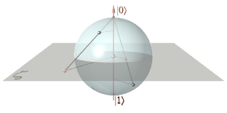
Inverse map may be written as
| (23) |
For concrete calculations it is better to work with usual pair Eq. (20) instead of Eq. (22) with for . It is not possible to describe that using one map, i.e., such inverse construction for Eq. (21) may be expressed as atlas with two hemispheres
| (24) |
Both maps in atlas presented in Eq. (24) defined everywhere, except one pole of sphere and , respectively. For such definition on sphere without poles both maps Eq. (24) overlap, but differ on a phase multiplier
and so represent the same quantum state.
It is possible to use division of sphere using other value as threshold in Eq. (24), say in degenerate case second hemisphere contracts to single point on pole. But it is impossible to find a single continuous map due to some general theorem of differential geometry333 It was already mentioned, that the space of normalized complex vectors like Eq. (20) is equivalent to (hyper)sphere. For qubit it is and so Eq. (21) correspond to map . The map is well known as Hopf fibration and absence of continuous inverse map (section) follows from general theory of fiber bundles [28]..
It is convenient to consider a case with projectors “perpendicular to axis,” i.e., equator of Bloch sphere with and so due to Eq. (24)
| (25) |
4.3 Measurement of Bell pair
Let us now consider measurements of two qubits in singlet state Eq. (15). The principle resembles different procedures with P-measurement in Sec. 3.2.
Let us for simplicity to consider for both systems only measurements described by projectors Eq. (19) with and states Eq. (25). For such a kind of states it is simple to calculate scalar products with Bell state Eq. (15)
and standard expression for probabilities444The expression with is valid for arbitrary states (without limitation ).
| (28) |
Any pair of states and is the basis in two-dimensional Hilbert space. Four projectors describe measurement procedure for system with two parts. Probabilities of four different outcomes are described by Eq. (28), i.e., or
| (29) |
Projectors and describe “partial” measurements on first and second subsystem respectively. Here situation is similar with measurement of components, because the operators also have degenerate eigenspaces.
Formally Eq. (29) show, that probabilities to find subsystems in two different states are equal , and the same with second one . So results of measurements are correlated . It is usually considered correlator
| (30) |
The Eq. (30) describes “expectation value of the product of the two components,” [25] i.e., two components with values for measurement of spin along or opposite of given axes555It is denoted as in [8, 25] and as in [10]..
It is possible also to use procedure of P-measurement from Sec. 2 with application of to Bell state . It produces or with equal probabilities . If it to apply measurement after that, the final result of two such measurements is one of four states and Eq. (27) ensures, that probabilities are the same Eq. (29) as for simultaneous measurement of all values described earlier. The result is the same also if measurement is applied before .
So statistical results of the model do not depend on order of measurements and do not contradict relativity and locality, but simulation that on computer with random number generator has problems with the principles.
The Eq. (30) coincides with quantum mechanical expectation value and so any combinations with different orientations are in agreement with quantum mechanical description. E.g., Bell inequality in initial form [10, 25]
| (31) |
or more general version, CHSH (Clauser-Horne-Shimony-Holt) inequality [10, 26]
| (32) |
must be violated for some directions.
Such agreement with quantum mechanical description is produced by formal nonlocality. Really already description of state by single array of complex numbers with four component used in model Sec. 2 is hardly may be treated as local.
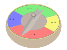
Model of measurement procedure is also not local, for example for description of simultaneous measurement of both systems should be used single random number for generating of four probabilities Eq. (29). It is similar with single roulette (Fig. 5) with four sectors (with angles , , , ), when given sector corresponds to appearance of pair of values for two distant measurements.
On the other hand, simulation of classical correlations also may use similar description, despite of locality of simulated physical system. But for classical case local description also exists.
The nonlocality is more obvious for separate measurements, then model Sec. 2 used above produces two outcomes like and after “partial” measurement. In computer simulation it is some intermediate result, hidden from a user of the program, but it just coincides with description of “instantaneous reduction,” criticized in EPR paper [23].
5 Conway-Kochen “Free Will” theorem
If to use two separate spin-1 systems, then combination of Kochen-Specker theorem with nonlocality complicates the picture.
Here is considered setup with more detailed physical model used in [11]. For each system is considered operators Eq. (5) and Eq. (6). Here they are written in symmetric form. Let us find precise expression for singlet state of two spin-1 systems with respect to such operators.
The singlet state should be invariant with respect to rotation of sphere in 3D Euclidean space used in physical model of Kochen-Specker theorem, i.e., ‘-sphere’ described in Sec. 3.2. It may be simply described using symmetric composition with two bases of the 3D real space Eq. (9)
| (33) |
because it is invariant with respect to Euclidean 3D rotations. It can be checked directly, that for any Eq. (33) may be rewritten using Eq. (6) as
and so expressed via eigenvectors Eq. (6) of any
| (34) |
It should be mentioned, that Eq. (33) and Eq. (34) are invariant only with respect to SO(3) subgroup of SU(3) group666 The difference of sign in first term of Eq. (34) with [11] is consequence of this fact..
Let us apply simultaneous N-measurement (here ) of state Eq. (34) with two different frames defined by eigenvectors of Eq. (9) and Eq. (11). Using representation of Eq. (33), and equation , it is possible to find decomposition for any basis
| (35) |
there are elements of transposed matrix Eq. (12). So the measurement produces up to nine outcomes with probabilities , but for description of experiments discussed in [11] such a fine decomposition is not required.
In [11] is considered case, when first experimenter measures full frame and second one only one direction. Let it be measurement of . It is possible to apply -measurement or P-measurement procedure from Sec. 2 for such scenario with projectors.
The results for both experimenters are:
i.e., results for always in agreement for both sides. The similar is true for measurement and , i.e., both experimenters got the same results for given axis.
Here is only three elements instead of nine in Eq. (35), because and commute and basis may be used for decomposition for both sides. It is not necessary even to know other elements of frame and for second experimenter to predict results of measurement.
Model of Sec. 2 may ensure such agreement with quantum mechanics due to ‘nonlocal roulette’ generating value of both measurements and alredy discussed in Sec. 4.3. So, example with two spin-1 systems discussed here does not differ much from consideration of Bell pair, or maybe even simpler, if to use model defined in Sec. 2.
In the main, model with two spins discussed in Conway-Kochen “Free Will” theorem [11] and some works on “quantum pseudotelepahy” [29] is interesting due to comparison with particular classical description. Really, it is possible to suggest a classical model that produces agreement, if for different frames second experimenter is using . Say, it is enough to use two equal programs on two distant computers with procedure Eq. (4) described in Sec. 3.1. With same value of pseudo-random number generator both users will have the same results for the frames with the same . On the other hand, Kochen-Specker theorem ensures, that such a method fails, if second user may choose also or axis, e.g., to use second or third outcome in Eq. (4).
The problem is similar with contextuality due to hidden dependence in algorithms like Eq. (4) from value already discussed in Sec. 3.1. Using two equivalent algorithms with pseudo-random numbers let reveal that, and Kochen-Specker theorem closes any possibility to escape777But formally, it is only no-go result for hidden variables models of the same classes, which are used in Bell, Kochen-Specker and Conway-Kochen models. It may be risky to be absolutely sure, that any local classical model will not work, because history of no-go theorems about hidden variables have shown the appearance of new and new models, which were not taken into account by authors of no-go theorems.. So from classical point of view behavior of the quantum mechanical system (that anyway always produces the same results) is really miracle. Otherwise (without reference to the classical model) it is very similar with nonlocality problems associated with Bell pair and already discussed earlier in relation with “free will” [30].
6 Modified Deutsch-Hayden-Tipler model
Some conceptual problems with model in Sec. 2 were already mentioned. It maybe even possible to accept hidden internal nonlocality, that may not be found by any statistical test, but problem with relativity of order of events make the model nonconstructive.
There is interesting method to avoid problem with nonlocality and relativity discussed in [31, 32]. The papers use interpretation of quantum mechanics without reduction [33], but may be adapted for interpretation with “local reduction condition” to meet relativity principle. The basic idea, is that any measurement of correlation is possible only after final, local measurement, when some carriers with data about two nonlocal measurements in distant points are reunited.
It may be simply described using model Sec. 2. The basic tool for two distant measurement is non-perturbing measurement gate [5, 31] Fig. 6.
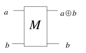
Really, in [31] was used Heisenberg representation of quantum computations [35]. Such representation has some advantages and formally was used already in [1], but it should be discussed elsewhere and here is used Schrödinger picture adopted in model Sec. 2.
The measurement gate is described by formula
| (36) |
where is addition modulo two. For such gate performs formal measurement in chosen (‘compuational’) basis, i.e., copies second state to the first one. Here note about computational basis is essential, because it is impossible to clone arbitrary state of [34].
Let us consider measurement of Bell pair.
At first step to each part ( and ) of distant pair are attached auxiliary qubits:
After application of non-destructive measurement gates Eq. (36) the state is
It is now possible to reunit auxiliary qubits in some local place
and perform destructive measurement that produces either or with equal probabilities.
From the one hand, such a picture does not have the problem with relativity of notion of simultaneous events discussed earlier, because qubits and are not separated. From the other one, presented elementary model hardly could be considered as local, because state of whole nonlocal system with four qubits after final measurement is changed instantly. Similar models in [31, 32] are local, because any destructive measurements (‘collapse of wave function’) are forbidden.
A simple way to avoid the last problem with nonlocality, is to use instead of measurement gate [31, 32] swap (exchange) gate (Fig. 7)
| (37) |
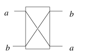
This gate exchanges any two states, not only basic ones, and not affected by no-cloning theorem. With application of such a gate the procedure of measurement discussed above becomes simpler:
First step
Second step (two distant ‘swap’-measurements)
Third step (reunion of and )
So even final destructive measurement, that produces with equal probabilities either or , does not affect on states of distant pair of qubits.
Acknowledgments and disclaimers
Author is grateful to participants of A. Friedmann Lab seminar (8 June 2006, St.-Petersburg, Russia) for comments and attention. This work is not made for hire and is not funded from any sources.
References
- [1] R. P. Feynman, “Simulating physics with computers,” Int. J. Theor. Phys. 21, 467–488 (1982).
- [2] A. S. Holevo, Statistical structure of quantum mechanics and hidden variables, (Znanie, Moscow 1985) [Russian].
- [3] A. A. Grib and R. R. Zapatrin, “Automata simulating quantum logics,” Int. J. Theor. Phys. 29, 113–123 (1990).
- [4] D. Deutsch, “Quantum theory, the Church-Turing principle and the universal quantum computer,” Proc. R. Soc. Lond. A 400, 97–117 (1985).
- [5] D. Deutsch, “Quantum computational networks,” Proc. R. Soc. Lond. A 425, 73–90 (1989).
- [6] D. Deutsch, R. Jozsa, “Rapid solution of problems by quantum computation,” Proc. R. Soc. Lond. A 439, 553–558 (1992).
- [7] P. W. Shor, “Algorithms for quantum computation: Discrete logarithms and factoring,” Proc. 35th Ann. Symp. FOCS, 124–134 (IEEE Comp. Soc. Press, Los Alamitos 1994).
- [8] J. S. Bell, Speakable and unspeakable in quantum mechanics, (Cambridge University Press, Cambridge, 1987).
- [9] S. Kochen and E. Specker, “The problem of hidden variables in quantum mechanics,” J. of Math. and Mech. 17 59–87 (1967).
- [10] A. Peres, Quantum theory: concepts and methods, (Kluwer Academic Publishers, Dordrecht 1993).
- [11] J. Conway and S. Kochen, “The Free Will theorem,” quant-ph/0604079.
- [12] P. A. M. Dirac, The principles of quantum mechanics, (Oxford University Press, Oxford 1958).
-
[13]
J. von Neumann, Mathematische Grundlagen der Quantenmechanik,
(Verlag von Julius Springer, Berlin 1932),
English version: Mathematical foundations of quantum mechanics, (Princeton University Press, Princeton, NJ, 1955). -
[14]
D. Aharonov, “Quantum computation — a review,” In D. Stauffer (ed),
Annual Review of Computational Physics, volume VI (1998);
quant-ph/9812037.
J. Preskill, Lecture notes for Physics 229: Quantum information and computation, (Calif. Inst. Tech., Pasadena 1998);
URL: http://www.theory.caltech.edu/people/preskill/ph229. -
[15]
D. Aharonov, A. Y. Kitaev, and N. Nisan,
“Quantum circuits with mixed states,”
in Proc. 30th Ann. ACM STOC, 20–30 (ACM Press, New York 1998);
quant-ph/9806029.
M. Keyl, “Fundamentals of quantum information theory”, Phys. Rep. 369, 431–548 (2002); quant-ph/0202122. -
[16]
T. Kohonen, Self-organizing maps, (Springer-Verlag, New York 2001).
G. Winkler, Image analysis, random fields and dynamic Monte Carlo methods, (Springer-Verlag, New York 1995). -
[17]
D. A. Meyer, “Finite precision measurement nullifies the Kochen-Specker theorem,”
Phys. Rev. Lett. 83, 3751–3754 (1999);
quant-ph/9905080.
A. Kent, “Hidden variables are compatible with physical measurements,” Phys. Rev. Lett. 83, 3755–3757 (1999); quant-ph/9906006.
R. K. Clifton and A. Kent, “Simulating quantum mechanics by non-contextual hidden variables”, Proc. R. Soc. Lond. A 456, 2101–2114 (2000); quant-ph/9908031. - [18] A. Peres, “What’s wrong with these observables?”, Found. Phys. 33, 1543–1547 (2003); quant-ph/0207020.
- [19] J. Barrett and A. Kent, “Non-contextuality, finite precision measurement and the Kochen-Specker theorem”, Stud. Hist. Philos. Mod. Phys. 35, 151–176 (2004); quant-ph/0309017.
- [20] D. M. Appleby, “The Bell-Kochen-Specker theorem,” Stud. Hist. Philos. Mod. Phys. 36, 1–28 (2005); quant-ph/0308114.
- [21] M. G. Kendall and P. A. P. Morran, Geometrical probability, (Griffin, London 1963).
- [22] M. Gardner, “Probability and ambiguity,” in The second Scientific American book of mathematical puzzles and diversions, (Simon & Schuster, New York 1961; University of Chicago Press, 1987).
- [23] A. Einstein, B. Podolsky, and N. Rosen, “Can quantum-mechanical description of physical reality be considered complete?”, Phys. Rev. 47, 777–780 (1935).
- [24] J. S. Bell, “On the Einstein-Podolsky-Rosen paradox,” Physics 1, 195–200 (1964); reprinted in [8] pp 14–21.
- [25] J. S. Bell, “On the problem of hidden variables in quantum mechanics”, Rev. Mod. Phys. 38, 447–452 (1966); reprinted in [8] pp 1–13.
- [26] J. F. Clauser, M. A. Horne, A. Shimony, and R. A. Holt, “Proposed experiment to test local hidden-variable theories,” Phys. Rev. Lett. 23, 880–884 (1969).
- [27] R. Penrose and W. Rindler, Spinors and space-time, Vol I, Two-spinors calculus and relativistic fields, (Cambridge University Press, Cambridge 1986).
- [28] N. Steenrod, The topology of fiber bundles, (Princeton University Press, Princeton 1951).
- [29] G. Brassard, A. Broadbent, and A. Tapp, “Quantum pseudo-telepathy,” Found. Phys. 35, 1877–1907 (2005); quant-ph/0407221.
- [30] A. Peres, “Existence of ‘free will’ as a problem of physics,” Found. Phys. 16, 573–584 (1986).
- [31] D. Deutsch and P. Hayden, “Information flow in entangled quantum systems,” Proc. R. Soc. Lond. A 456, 1759–1774 (2000); quant-ph/9906007.
- [32] F. J. Tipler, “Does quantum nonlocality exist? Bell’s theorem and the many-worlds interpretation,” quant-ph/0003146.
- [33] H. Everett III, ‘ “Relative state” formulation of quantum mechanics,’ Rev. Mod. Phys. 29, 454–462 (1957).
- [34] W. K. Wootters and W. H. Zurek, “A single quantum cannot be cloned,” Nature 299, 802–803 (1982).
- [35] D. Gottesman, “The Heisenberg representation of quantum computers,” in S. P. Corney, R. Delbourgo, and P. D. Jarvis (eds), Group 22: Proc. XXII Inter. Colloq. on Group Theor. Methods in Physics, 32–43 (International Press, Cambridge, MA, 1999); quant-ph/9807006.