The entanglement of damped noon-state and its performance in phase measurement

Abstract

The state evolution of the initial optical noon state is investigated. The residue entanglement of the state is calculated after it is damped by amplitude and phase damping. The relative entropy of entanglement of the damped state is exactly obtained. The performance of direct application of the damped noon state is compared with that of firstly distilling the docoherence damped state then applying it in measurement.

1 Introduction

Quantum entanglement between two or more particles has attracted great interest and produced many applications in quantum information processing, such as quantum communication,quantum computation and quantum cryptography and quantum metrology. It has been known for some time that entangled states can be used to perform supersensitive measurements, for example in optical interferometry or atomic spectroscopy[1] [2] [3]. The idea has been demonstrated for entangled states of two photons[4], three photons [5] and four photons [6]. In the best case, the interferometric sensitivity can reach the quantum mechanical ’Heisenberg-limit’ in entanglement enhanced measurement which overwhelms the classical shot noise limit. If $\phi$ is the phase to be estimated, and $N$ is the number of independent trials in the estimation, the classical shot noise limit is $\Delta\phi=1/\sqrt{N}.$ When entangled state is used, the limit can be reduced to at most to ’Heisenberg-limit’ $\Delta\phi=1/N$. One of such entangled states is the so-called noon state

$$\left|N::0\right\rangle_{ab}=\frac{1}{\sqrt{2}}(\left|N,0\right\rangle_{ab}+\left|0,N\right\rangle_{ab})$$ (1)

which describes two modes $a,b$ in a superposition of distinct Fock states $\left|n_{a}=N,n_{b}=0\right\rangle$ and $\left|n_{a}=0,n_{b}=N\right\rangle.$ The applications of this state include quantum metrology [1] [2] [3] [7] and quantum lithography [8]. In all the applications of noon state, the decoherence of the state and the performance of the damped state are less concerned. Huelga et al considered the ion system in presence of decoherence[9]. It is inevitable that quantum state interacts with environment which will cause the decoherence of the state, thus in quantum supersensitive measurements decoherence should be included. We in this paper will investigate the entanglement of optical noon state in presence of decoherence and the performance degradation.

2 Decoherence

A quantum state will undergo decoherence after preparation. The decoherece comes from the interaction with environment. For continuous variable (CV) system, two most popular decoherences are amplitude damping and phase damping. The master equation describing these two decoherences for the density operator $\rho$ is [10] [11][12] (in the interaction picture) $\frac{d\rho}{dt}=(\mathcal{L}_{1}\mathcal{+L}_{2})\rho,$with $\mathcal{L}_{1}$ represents the amplitude damping concerning with vacuum environment,

$$\mathcal{L}_{1}\rho=\sum_{i}\frac{\Gamma_{i}}{2}(2a_{i}\rho a_{i}^{\dagger}-a_{i}^{\dagger}a_{i}\rho-\rho a_{i}^{\dagger}a_{i}),$$ (2)

and $\mathcal{L}_{2}$ represents the phase damping,

$$\mathcal{L}_{2}\rho=\sum_{i}\frac{\gamma_{i}}{2}[2a_{i}^{\dagger}a_{i}\rho a_{i}^{\dagger}a_{i}-(a_{i}^{\dagger}a_{i})^{2}\rho-\rho(a_{i}^{\dagger}a_{i})^{2}],$$ (3)

with $a_{i}$ the annihilation operation of $i-th$ mode, and $\Gamma_{i}$ and $\gamma_{i}$ are damping coefficients of $i-th$ mode for amplitude and phase damping respectively. The solution to the master equation can be conveniently obtained by first transforming the equation to the diffusion equation of the characteristic function of the state, then solve the the differential equation of the characteristic function. The time evolution solution of he density operator can be recovered from the characteristic function.

The characteristic function is defined as $\chi=tr[\rho\mathcal{D}(\mu)]$, where $\mathcal{D}(\mu)=\exp(\mu a^{\dagger}-\mu^{*}a)$ is the displacement operator, with $\mu=[\mu_{1},\mu_{2},\cdots,\mu_{s}]$ $,a=[a_{1},a_{2},\cdots,a_{s}]^{T}$ and the total number of modes is $s$. The diffusion eqation of the characteristic function will be [13]

$$\frac{\partial\chi}{\partial t}=-\frac{1}{2}\sum_{j}\Gamma_{j}\{\left|\mu_{j}\right|\frac{\partial\chi}{\partial\left|\mu_{j}\right|}+\left|\mu_{j}\right|^{2})\chi\}+\frac{1}{2}\sum_{j}\gamma_{j}\frac{\partial^{2}\chi}{\partial\theta_{j}^{2}},$$ (4)

where $\mu_{j}=\left|\mu_{j}\right|e^{i\theta_{j}}.$ The solution is simply be

$$\chi(\mu,\mu^{*},t) = \int dx\chi(\mu e^{-\frac{\Gamma t}{2}+ix},\mu^{*}e^{-\frac{\Gamma t}{2}-ix},0)\prod_{j}(2\pi\gamma_{j}t)^{-1/2}$$

$$\exp[-\frac{x_{j}^{2}}{2\gamma_{j}t}-\frac{1}{2}(1-e^{-\Gamma_{i}t})\left|\mu_{j}\right|^{2}].$$

with $\mu e^{-\frac{\Gamma t}{2}+ix}$ standing for $(\mu_{1}e^{-\frac{\Gamma_{1}t}{2}+ix_{1}},\mu_{2}e^{-\frac{\Gamma_{2}t}{2}+ix_{2}},\cdots,\mu_{s}e^{-\frac{\Gamma_{s}t}{2}+ix_{s}})$. The time dependent state can be recovered by $\rho=\int[\prod_{j}\frac{d^{2}\mu_{j}}{\pi}]\chi(\mu,\mu^{*},t)D(-\mu)$ [14].

The characteristic function of the noon state is

$$\chi(\left|N::0\right\rangle) = \left\langle N::0\right|D(\mu)\left|N::0\right\rangle$$

$$= \frac{1}{2}e^{-\frac{\left|\mu\right|^{2}}{2}}[L_{N}(\left|\mu_{1}\right|^{2})+L_{N}(\left|\mu_{2}\right|^{2})+\frac{1}{N!}((-\mu_{1}^{*}\mu_{2})^{N}+(-\mu_{1}\mu_{2}^{*})^{N})].$$

where $L_{N}$ is the Laguerre polynomial of order $N:$ $L_{N}(z)=\sum_{m=0}^{N}\frac{(-z)^{m}}{m!}\binom{N}{m}.$ The time evolution of the characteristic function will be

$$\chi(\mu,\mu^{*},t) = \frac{1}{2}e^{-\frac{\left|\mu\right|^{2}}{2}}[L_{N}(\left|\mu_{1}\right|^{2}e^{-\Gamma_{1}t})+L_{N}(\left|\mu_{2}\right|^{2}e^{-\Gamma_{2}t})$$

$$+\frac{1}{N!}e^{-N\overline{\Gamma}t-N^{2}\overline{\gamma}t}((-\mu_{1}^{*}\mu_{2})^{N}+(-\mu_{1}\mu_{2}^{*})^{N})],$$

where $\overline{\Gamma}=\frac{1}{2}(\Gamma_{1}+\Gamma_{2}),$ $\overline{\gamma}=\frac{1}{2}(\gamma_{1}+\gamma_{2}).$ The solution to the master equation of density operator will be

$$\rho = \frac{1}{2}\{\sum_{m=0}^{N}\binom{N}{m}[(1-e^{-\Gamma_{1}t})^{N-m}e^{-m\Gamma_{1}t}\left|m0\right\rangle\left\langle m0\right|$$

$$+(1-e^{-\Gamma_{2}t})^{N-m}e^{-m\Gamma_{2}t}\left|0m\right\rangle\left\langle 0m\right|]$$

$$+e^{-N\overline{\Gamma}t-N^{2}\overline{\gamma}t}[\left|N0\right\rangle\left\langle 0N\right|+\left|0N\right\rangle\left\langle N0\right|]\}.$$

The integral on $\mu$ is carried out by the technique of integral within ordered operators.

3 The entanglement of the damped state

The damped state $\rho$ is a mixed state. According to Peres-Horodecki criterion, the state is always entangled. The entanglement of the state can be carried out if measured by relative entropy of entanglement. The relative entropy of $\rho$ with respect to a separable state $\sigma$ is $S(\rho\left\|\sigma\right.)=Tr(\rho\log_{2}\rho-\rho\log_{2}\sigma)$, the relative entropy of entanglement of $\rho$ is the minimization of $S(\rho\left\|\sigma\right.)$ over all separable state $\sigma.$ Let the extremal separable state that minimizes the relative entropy be $\sigma^{*}$. Denote $\rho=c_{00}\left|00\right\rangle\left\langle 00\right|+\sum_{m=1}^{N}(c_{m0}\left|m0\right\rangle\left\langle m0\right|+$ $c_{0m}\left|0m\right\rangle\left\langle 0m\right|)$ $+c(\left|N0\right\rangle\left\langle 0N\right|+\left|0N\right\rangle\left\langle N0\right|)$. We will obtain $\sigma^{*}$ by first suppose $\sigma^{*}$ having a special form then prove that $\sigma^{*}$ is extremal (see Appendix) . Suppose

$$\sigma^{*} = d_{00}\left|00\right\rangle\left\langle 00\right|+\sum_{m=1}^{N}(d_{m0}\left|m0\right\rangle\left\langle m0\right|+d_{0m}\left|0m\right\rangle\left\langle 0m\right|)$$

$$+d(\left|N0\right\rangle\left\langle 0N\right|+\left|0N\right\rangle\left\langle N0\right|)+d_{NN}\left|NN\right\rangle\left\langle NN\right|.$$

The function that should be minimized is

$$-Tr(\rho\log_{2}\sigma^{*}) = -c_{00}\log_{2}d_{00}-\sum_{m=1}^{N-1}(c_{m0}\log_{2}d_{m0}+c_{m0}\log_{2}d_{m0})$$ (15)

$$-Tr\left[\begin{array}[]{ll}c_{N0}&c\\ c&c_{0N}\end{array}\right]\log_{2}\left[\begin{array}[]{ll}d_{N0}&d\\ d&d_{0N}\end{array}\right].$$

The constraints are $Tr\sigma^{*}=1$ and $d^{2}=d_{00}d_{NN}$ , the later specifies that the extremal separable state should be at the edge of the separable state set (e.g.[15]). For the general situation of $c_{N0}\neq c_{0N},$ the minimization problem have not an analytical solution[16]. When the amplitude damping is symmetric, we have $\Gamma_{1}=\Gamma_{2}=\Gamma$ $($thus $c_{m0}=c_{0m};$ $m=1,\cdots,N),$ the solution to the minimization problem is

$$d_{m0} = d_{0m}=c_{0m,}\text{ for }m=1,\cdots,N-1;$$ (16)

$$d_{00} = \frac{(c_{N0}+c_{00})^{2}c_{00}}{(c_{N0}+c_{00})^{2}-c^{2}};\text{ }d_{NN}=\frac{c^{2}c_{00}}{(c_{N0}+c_{00})^{2}-c^{2}};$$ (17)

$$d_{0N} = d_{N0}=c_{N0}-d_{NN};\text{ }d=\frac{c(c_{N0}+c_{00})c_{00}}{(c_{N0}+c_{00})^{2}-c^{2}};$$ (18)

The relative entropy of entanglement of state $\rho$ is: $E_{r}(\rho)$ $=Tr\rho(\log_{2}\rho-\log_{2}\sigma^{*})=c_{00}\log\frac{c_{00}}{d_{00}}+c_{+}\log\frac{c_{+}}{d_{+}}$ $+c_{-}\log\frac{c_{-}}{d_{-}},$ with $c_{\pm}=c_{N0}\pm c,$ $d_{\pm}=d_{N0}\pm d$. It can be written as

$$E_{r}(\rho)=2(c_{00}+c_{N0})[1-H_{2}(\frac{c_{00}+c_{N0}+c}{2(c_{00}+c_{N0})})],$$ (19)

where $H_{2}(\varepsilon)=-\varepsilon\log_{2}\varepsilon-(1-\varepsilon)\log_{2}(1-\varepsilon)$ is the binary entropy function, and $c_{00}=(1-e^{-\Gamma t})^{N},$ $c_{N0}=\frac{1}{2}e^{-N\Gamma t},c=\frac{1}{2}e^{-N\Gamma t-N^{2}\overline{\gamma}t}$. It should be mentioned that the corresponding solution to the problem of two qubits system is known [17] [16].

Other entanglement measures are entanglement of formation and distillable entanglement. From the definition of the entanglement of formation, it is easily to obtained an upper bound for the entanglement of formation, which is

$$E_{f}^{+}(\rho)=(c_{N0}+c_{0N})H_{2}(\frac{1+\sqrt{1-c^{2}/(c_{N0}+c_{0N})^{2}}}{2}).$$ (20)

We suspect if this is just the entanglement of formation itself. For the symmetric amplitude damping, when there is not phase damping and $N\geq 5,$ $E_{f}^{+}(\rho)$ is very close to $E_{r}(\rho).$

The distillable entanglement is lower bounded by the coherent information (hashing inequality). The coherent information of the state is

$$I_{c}(\rho) = -c_{N0}\log_{2}c_{N0}-(\sum_{m=1}^{N}c_{0m})\log_{2}(\sum_{m=1}^{N}c_{0m})$$

$$+\sum_{m=1}^{N-1}c_{0m}\log_{2}(c_{0m})+c_{+}\log_{2}c_{+}+c_{-}\log_{2}c_{-}.$$

When only phase damping is considered, that is $\Gamma_{1}=\Gamma_{2}=0,$ we have $c_{0m}=0$ for all $m<N,$ $c_{N0}=\frac{1}{2},c=\frac{1}{2}e^{-N^{2}\overline{\gamma}t}.$ The coherent information will be $I_{c}(\rho)=1-H_{2}(\frac{1}{2}+\frac{1}{2}e^{-N^{2}\overline{\gamma}t}).$ Meanwhile the relative entropy of entanglement will also be $E_{r}(\rho)=1-H_{2}(\frac{1}{2}+\frac{1}{2}e^{-N^{2}\overline{\gamma}t}).$ Because distillable entanglement $E_{d}(\rho)$ is upper bounded by the relative entropy of entanglement, we have $I_{c}(\rho)\leq E_{d}(\rho)\leq E_{r}(\rho)$. Now $I_{c}(\rho)=E_{r}(\rho)$, thus for the situation only phase damping, the distillable entanglement is:

$$E_{d}(\rho)=1-H_{2}(\frac{1}{2}+\frac{1}{2}e^{-N^{2}\overline{\gamma}t}).$$ (22)

4 Performance of damped state in entanglement enhanced phase measurement

In the entanglement enhanced phase measurement, the measurement operator is $A=\left|N0\right\rangle\left\langle 0N\right|+\left|0N\right\rangle\left\langle N0\right|$[5]. We suppose the state undergo the phase shift just before the measurement apparatus. The state is modified by the phase shift to $\rho_{\varphi}=c_{00}\left|00\right\rangle\left\langle 00\right|+\sum_{m=1}^{N}(c_{m0}\left|m0\right\rangle\left\langle m0\right|+$ $c_{0m}\left|0m\right\rangle\left\langle 0m\right|)$ $+c(e^{iN\varphi}\left|N0\right\rangle\left\langle 0N\right|+e^{-iN\varphi}\left|0N\right\rangle\left\langle N0\right|).$ It should be noted that the relative entropy of entanglement is not changed by the phase shift[16]. Thus $\left\langle A\right\rangle=Tr\rho_{\varphi}A=$ $2c\cos N\varphi=$ $e^{-N\overline{\Gamma}t-N^{2}\overline{\gamma}t}\cos N\varphi,$ $\Delta A=\sqrt{\left\langle A^{2}\right\rangle-\left\langle A\right\rangle^{2}},$ the phase deviation is

$$\Delta\varphi=\frac{\Delta A}{\left|\partial\left\langle A\right\rangle/\partial\varphi\right|}=\frac{\sqrt{\frac{1}{2}(e^{-N\Gamma_{1}t}+e^{-N\Gamma_{2}t})-e^{-2N\overline{\Gamma}t-2N^{2}\overline{\gamma}t}\cos^{2}N\varphi}}{Ne^{-N\overline{\Gamma}t-N^{2}\overline{\gamma}t}\left|\sin N\varphi\right|}.$$ (23)

The minimal $\Delta\varphi$ will be at $\varphi=(2k+1)\frac{\pi}{2N}.$ Thus the bset phase measurement precision will be

$$(\Delta\varphi)_{best}=\frac{1}{N}e^{N^{2}\overline{\gamma}t}\sqrt{\frac{1}{2}(e^{N\Gamma_{1}t}+e^{N\Gamma_{2}t})}.$$ (24)

We may adopt another strategy to enhance the phase measurement precision with the mixed entangled state at hand. In this strategy, the damped state $\rho$ is distilled to noon state, then we use the new noon state for measurement. The successful probability of distilling a noon state from the damped state is characterized by the distillable entanglement of $\rho.$ Thus we use noon state in the measurement at a probability of $p=E_{d}(\rho)$, the phase deviation is the Heisenberg limit $(\Delta\varphi)_{q}=\frac{1}{N}$; In a probability of $1-E_{d}(\rho)$ we have no quantum entanglement to enhance the measurement, the phase deviation will be the classical shot noise limit $(\Delta\varphi)_{c}=\frac{1}{\sqrt{N}}.$ The mixture of the two kind of measurements will have the phase deviation: $(\Delta\varphi)_{d}=\sqrt{p(\Delta\varphi)_{q}^{2}+(1-p)(\Delta\varphi)_{c}^{2}},$ (this may derived from the fact that the mixture probability distribution function $f_{d}(\varphi)=pf_{q}(\varphi)+(1-p)f_{c}(\varphi),$ with $f_{q}(\varphi)$ and $f_{c}(\varphi)$ are probability distribution function of entanglement enhanced phase measurement and classical measurement, the two kinds of measurement have the same mean). In the distillation strategy, the phase deviation will be

$$(\Delta\varphi)_{d}=\sqrt{E_{d}/N^{2}+(1-E_{d})/N}.$$ (25)

We can compare the performances of the direct application of damped state to phase measurement and the distillation then measurement strategy. Let us firstly consider the situation of phase damping alone. We have

$$\frac{(\Delta\varphi)_{d}^{2}}{(\Delta\varphi)_{best}^{2}}=[1+(N-1)H_{2}(\frac{1}{2}+\frac{1}{2}e^{-N^{2}\overline{\gamma}t})]e^{-2N^{2}\overline{\gamma}t}.$$ (26)

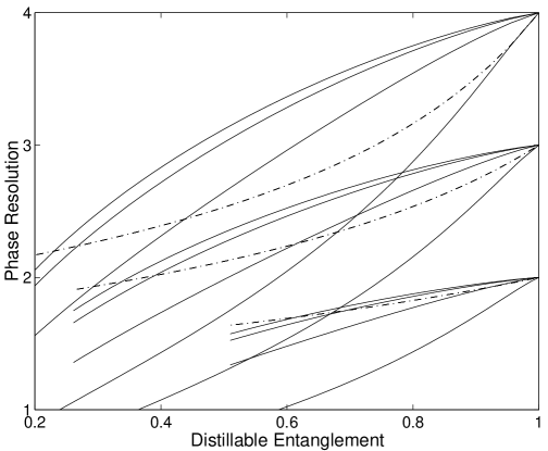
Figure 1: The performance of state with phase damping alone in entanglement enhanced measurement. The phase resolution is defined as the inverse of phase deviation. The line groups from top to bottom are for $N=4,3,2$ respectively. In each group the solid lines from top to bottom are $1/\Delta\varphi$ for $\varphi=(1,3/4,1/2,1/4)\pi/(2N)$ respectively, the dashed line is for $1/(\Delta\varphi)_{d}$.

As indicated in figure 1, the performance of direct application is better when the phase $\varphi$ under measurement is near $(2k+1)\pi/(2N)$. While distillation strategy is better when the phase $\varphi$ is far from these values.

In the amplitude damping situation, distillable entanglement is upper and lower bounded by the relative entropy of entanglement and the coherent information respectively. It is followed that the phase deviation is also upper and lower bounded. We have $(\Delta\varphi)_{dl}\leq(\Delta\varphi)_{d}\leq(\Delta\varphi)_{du}$ with $(\Delta\varphi)_{dl}=\sqrt{E_{r}/N^{2}+(1-E_{r})/N}$ and $(\Delta\varphi)_{du}=\sqrt{I_{c}/N^{2}+(1-I_{c})/N}.$ In figure 2, we calculate the upper and lower bounds of resolution for the distillation strategy in situation of symmetric amplitude damping alone. We can see that the best resolution of the direct application of damped state is better than the distillation strategy.

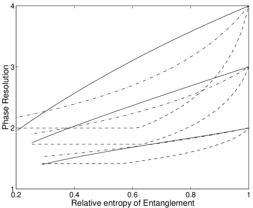
Figure 2: The performance of state with amplitude damping alone in entanglement enhanced measurement. The phase resolution is defined as the inverse of phase deviation. The line groups from top to bottom are for $N=4,3,2$ respectively. In each group the solid line is for $1/(\Delta\varphi)_{best}$, the dotdash line is for $1/(\Delta\varphi)_{dl}$,the dashed line is for $1/(\Delta\varphi)_{du}$.

5 Conclusions

The master equation of quantum continuous variable system is sovled in the case of simultaneous amplitude damping of vacuum environment and phase damping. When the initial state is a noon state, the exact expression of time dependent solution of density operator is obtained via the characteristic function method. An analytical formula is given for the relative entropy of entanglement of the damped state when the two modes of the noon state undergo the same amount of amplitude damping. In the asymmetric amplitude damping, the the relative entropy of entanglement can be calculated by numerically solving a group of algebraic equations. In the situation of phase damping alone, the exact distillable entanglement is given, which enables the comparison of two strategies of applying the damped state in phase measurement possible. When amplitude damping is present, we calculate the relative entropy of entanglement and coherent information of the damped state. We use these to specify the upper and lower bounds of the distillable entanglement.

The performance of direct application of the damped state in phase measurement is better than that of firstly distilling the damped state then applying it in measurement when the phase under estimation is near $(2k+1)\pi/(2N)$. While distillation strategy is better when the phase $\varphi$ is far from these values.

Appendix: Proof of the extremal state

We prove that $\sigma^{*}$ is extremal by the fact that local minimum is also the global minimum when it is in regard to the relative entropy of entanglement[18]. Hence we only need to prove that $\sigma^{*}$ is the local minimal state. Let $f(x,\sigma^{*},\sigma)=S(\rho\left\|(1-x)\sigma^{*}+x\sigma\right.)$ be the relative entropy of a state obtained by moving from $\sigma^{*}$ towards some $\sigma$. The derivative of $f$ will be [19][18]

$$\frac{\partial f}{\partial x}\left(0,\sigma^{*},\sigma\right)=\int_{0}^{\infty}((\sigma^{*}+t)^{-1}\rho(\sigma^{*}+t)^{-1}\delta\sigma)dt=TrB\delta\sigma,$$

where we denote $(1-x)\sigma^{*}+x\sigma=\sigma^{*}-\delta\sigma,$ and the operator $B$ has the following matrix elements in the eigenbasis $\{\left|\chi_{n}\right\rangle\}$ of $\sigma^{*}$:

$$B_{mn}^{\chi}=\left\langle\chi_{m}\right|B\left|\chi_{n}\right\rangle=\frac{\log\chi_{n}-\log\chi_{m}}{\chi_{n}-\chi_{m}}\left\langle\chi_{m}\right|\rho\left|\chi_{n}\right\rangle.$$

And when $\chi_{m}=\chi_{n}$, the corresponding coefficient should be replaced with the limit value of $\chi_{n}^{-1}.$

We should prove that for any separable state $\chi$,

$$\frac{\partial f}{\partial x}\left(0,\sigma^{*},\sigma\right)=TrA\delta\sigma=TrA(\sigma^{*}-\sigma)\geq 0.$$

where $TrB\sigma^{*}=1$[19], But any $\sigma\in\mathcal{D}$ (separable state set) can be written in the form of $\sigma=\sum_{i}p_{i}\left|\alpha^{i}\beta^{i}\right\rangle\left\langle\alpha^{i}\beta^{i}\right|$ and so $\frac{\partial f}{\partial x}\left(0,\sigma^{*},\sigma\right)=\sum_{i}p_{i}\frac{\partial f}{\partial x}\left(0,\sigma^{*},\left|\alpha^{i}\beta^{i}\right\rangle\left\langle\alpha^{i}\beta^{i}\right|\right)$, The problem is reduced to prove that for any normalized pure state $\left|\alpha\beta\right\rangle\left\langle\alpha\beta\right|,$

$$\left\langle\alpha\beta\right|B\left|\alpha\beta\right\rangle\leq 1.$$ (A1)

We here prove the situation of symmetric amplitude damping system, the more general proof for corresponding two qubits system was already been found[16], and the proof of asymmetric amplitude damping system is similar to that of two qubits system. For symmetric amplitude damping , the operator

$$B = \frac{c_{00}}{d_{00}}\left|00\right\rangle\left\langle 00\right|+\sum_{m=1}^{N-1}(\left|m0\right\rangle\left\langle m0\right|+\left|0m\right\rangle\left\langle 0m\right|)$$

$$+\frac{1}{2}(\frac{c_{+}}{d_{+}}+\frac{c_{-}}{d_{-}})(\left|N0\right\rangle\left\langle N0\right|+\left|0N\right\rangle\left\langle 0N\right|)+\frac{1}{2}(\frac{c_{+}}{d_{+}}-\frac{c_{-}}{d_{-}})(\left|N0\right\rangle\left\langle 0N\right|+\left|0N\right\rangle\left\langle N0\right|).$$

Denote $\left|\alpha\right\rangle=\sum_{m}\alpha_{m}\left|m\right\rangle,$ thus $\left\langle\alpha\beta\right|B\left|\alpha\beta\right\rangle=\frac{c_{00}}{d_{00}}\left|\alpha_{0}\beta_{0}\right|^{2}+\sum_{m=1}^{N-1}(\left|\alpha_{m}\beta_{0}\right|^{2}+\left|\alpha_{0}\beta_{m}\right|^{2})$ $+\frac{1}{2}(\frac{c_{+}}{d_{+}}+\frac{c_{-}}{d_{-}})(\left|\alpha_{0}\beta_{N}\right|^{2}+\left|\alpha_{N}\beta_{0}\right|^{2})+\frac{1}{2}(\frac{c_{+}}{d_{+}}-\frac{c_{-}}{d_{-}})(\alpha_{N}\beta_{0}\alpha_{0}^{*}\beta_{N}^{*}+\alpha_{0}\beta_{N}\alpha_{N}^{*}\beta_{0}^{*}).$ Let $K_{1}=1-\sum_{m=1}^{N-1}\left|\alpha_{m}\right|^{2}$ ,$K_{2}=1-\sum_{m=1}^{N-1}\left|\beta_{m}\right|^{2},$ (with $0\leq K_{1},K_{2}\leq 0),$ and $\alpha_{0}=\sqrt{K_{1}}\cos\theta_{1},\alpha_{N}=\sqrt{K_{1}}\sin\theta_{1}e^{i\eta_{1}},$ $\beta_{0}=\sqrt{K_{2}}\cos\theta_{2}e^{i\eta_{2}},$ $\beta_{N}=\sqrt{K_{2}}\sin\theta_{2}e^{i\eta_{3}}.$ Denote $\eta=\eta_{2}-\eta_{1}-\eta_{3}$, after maximization on $\eta$, we have

$$\left\langle\alpha\beta\right|B\left|\alpha\beta\right\rangle = \frac{c_{00}}{d_{00}}K_{1}\cos^{2}\theta_{1}\cos^{2}\theta_{2}+(1-K_{1})K_{2}\cos^{2}\theta_{2}+(1-K_{2})K_{1}\cos^{2}\theta_{1}$$

$$+\frac{c_{+}}{2d_{+}}K_{1}K_{2}\sin^{2}(\theta_{1}+\theta_{2})+\frac{c_{-}}{2d_{-}}K_{1}K_{2}\sin^{2}(\theta_{1}-\theta_{2}).$$

Suppose the extremal value is achieved at some $K_{1}\neq 0,1,$ by derivative on $K_{1},$ we obtain the supposed (may not exist) extremal value $\left\langle\alpha\beta\right|B\left|\alpha\beta\right\rangle=K_{2}\cos^{2}\theta_{2}\leq 1.$ What left is to verify that when $K_{1},K_{2}=0$ or $1,$ $\left\langle\alpha\beta\right|B\left|\alpha\beta\right\rangle$ will not exceeds $1$. The nontrivial situation is $K_{1}=K_{2}=1,$ thus

$$\left\langle\alpha\beta\right|B\left|\alpha\beta\right\rangle=\frac{c_{00}}{4d_{00}}(\cos\phi_{1}+\cos\phi_{2})^{2}+\frac{c_{+}}{2d_{+}}\sin^{2}\phi_{1}+\frac{c_{-}}{2d_{-}}\sin^{2}\phi_{2},$$

where $\phi_{1,2}=\theta_{1}\pm\theta_{2}.$ By using the fact that $\frac{c_{00}}{d_{00}}(\frac{c_{+}}{d_{+}}+\frac{c_{-}}{d_{-}})=2\frac{c_{+}c_{-}}{d_{+}d_{-}},$ We can obtain the maximum value as

$$\left\langle\alpha\beta\right|B\left|\alpha\beta\right\rangle_{m}=\frac{1}{2}(\frac{c_{+}}{d_{+}}+\frac{c_{-}}{d_{-}})=1.$$

Hence inequality (A1) is proved. So that $\sigma^{*}$ is the extremal state that minimizes the relative entropy.

References

• [1] M. J. Holland and K. Burnett, Phys. Rev. Lett. 71, 1355(1993).
• [2] J. J. Bollinger, W. M. Itano, D. J. Wineland, and D. J.Heinzen, Phys. Rev. A 54, R4649 (1996).
• [3] J. P. Dowling, Phys. Rev. A 57, 4736 (1998).
• [4] M. D’Angelo, M.V. Chekhova, and Y. Shih, Phys. Rev. Lett. 87, 013602 (2001).
• [5] M. W. Mitchell, J. S. Lundeen, and A. M. Steinberg, Nature 429, 161 (2004).
• [6] P. Walther, J.-W. Pan, M. Aspelmeyer, R. Ursinand, S. Gasparoni, and A. Zeilinger, Nature 429, 158 (2004).
• [7] R. A. Campos, C. C. Gerry, and A. Benmoussa, Phys. Rev. A 68, 023810 (2003).
• [8] A.N. Boto, P. Kok, D.S. Abrams, S.L. Braunstein, C.P. Williams, and J.P. Dowling, Phys. Rev. Lett. 85, 2733 (2000); G.S. Agarwal, R.W. Boyd, E.M. Nagasako, and S.J. Bentley, Phys. Rev. Lett. 86, 1389 (2001).
• [9] S. F. Huelga, C. Macchiavello, T. Pellizzari, A. K. Ekert, M. B. Plenio, and J. I. Cirac, Phys. Rev. Lett. 79, 3865 (1997).
• [10] P. Kinsler and P. D. Drummond, Phys. Rev. A 43, 6194 (1991).
• [11] G. Lindblad, Commun. Math. Phys. 48, 119 (1976).
• [12] D. Walls and G. Milburn, Quantum optics (Springer Verlag, Berlin, 1994).
• [13] X.Y. Chen, Phys. Rev. A 73, 022307 (2006).
• [14] A. Perelomov, Generalized Coherent states, Springer Verlag, Berlin (1986).
• [15] X.Y. Chen, Phys. Rev. A 71, 062320 (2005).
• [16] X.Y. Chen, L. M. Meng, L. Z. Jiang, and X. J. Li, Chin.Phys. Lett 22, 2755 (2005).
• [17] V.Vedral, M. B. Plenio Phys. Rev. A 57,1619 (1998).
• [18] V. Vedral, M. B. Plenio , K. Jacobs and P. L. Knight, Phys. Rev. A 56, 4452 (1997).
• [19] J. Řeháček and Z. Hradil, Phys. Rev. Lett. 90, 127904 (2003).