Always On Non-Nearest-Neighbor Coupling in Scalable Quantum Computing

Abstract

We study the non-nearest-neighbor interaction effect in $1$-D spin-$1/2$ chain model. In many previous schemes this long-range coupling is omitted because of its relative weak strength compared with the nearest-neighbor coupling. We show that the quantum gate deviation induced by the omitted long-range interaction depends on not only its strength but also the scale of the system. This implies that omitting the long-range interaction may challenge the scalability of previous schemes. We further propose a quantum computation scheme. In this scheme, by using appropriate encoding method, we effectively negate influence of the next-nearest-neighbor interaction in order to improve the precision of quantum gates. We also discuss the feasibility of this scheme in $1$-D Josephson charge qubit array system. This work may offer improvement in scalable quantum computing.

I Introduction

One of the critical problems in realizing scalable quantum computation (QC) is performing two qubits gates, which implies that the couplings between qubits are variable functions subject to external control. In many physical systems, this requirement is not easy to be satisfied. Recently various “always on” QC schemes have been proposed to solve this problem. Zhou et al. suggest encoding logical qubits in interaction free subspace (IFS) Zhou1 Zhou2 , while Benjamin et al. suggest changing interaction type between qubits from non-diagonal Heisenberg type to diagonal Ising type by tuning the Zeeman energy splits of individual qubits Bose1 . Schemes implementing above ideas into AFM spin ring and optical systems have already been developed Troiani Lovett .

These above elegant proposals mainly concern a $1$-D spin-$1/2$ chain with couplings between neighboring qubits. This model is a good analogue to many candidate scalable QC implementations. But in realistic systems such as quantum dot and optical lattice, there is not only the nearest-neighbor interaction, but also the next-nearest-neighbor, or even longer range interactions existing. In this paper we study effect of the non-nearest-neighbor coupling in $1$-D spin-$1/2$ chain model. Since the strength of the long-range coupling is often much smaller than that of the nearest-neighbor coupling, in many previous schemes its effect was ignored. But this omission results deviation in performing quantum gates. In this paper first we estimate the deviation of quantum gates induced by the omitted long-range interaction. Results imply that this deviation depends on not only the long-range interaction strength but also the length of the spin chain. This means that though the long-range interaction strength is very small, the induced deviation can “cumulate” on the whole $1$-D spin-$1/2$ chain, hence scalability of previous QC scheme is restricted. Following this estimation, we consider how to suppress this unwanted effect. We propose a QC scheme in which by using proper encoding methods, influence of the perpetual next-nearest-neighbor interaction is effectively negated, hence the precision of quantum gates updated. Compared with previous schemes in which the long-range coupling was omitted, our scheme does not cause the speed of quantum gates slow evidently. We also discuss the feasibility of this scheme in $1$-D Josephson charge qubit array system.

This paper is organized as follow: In the second section we consider a $1$-D spin-$1/2$ chain model. In the recent “always-on” QC schemes Zhou2 Bose1 , long-range interaction terms are always neglected. Here, we estimate the quantum gates deviation induced by an omitted perpetual next-nearest-neighbor Ising type interaction term. In the third section we consider how to suppress influence of the untunable long-range coupling. We use “blockade spin” encoding method to effectively neutralize unwanted influence of the perpetual next-nearest-neighbor interaction. Based on this encoding method we propose a QC scheme. In the fourth section we study the feasibility of this scheme in $1$-D Josephson junction charge qubit array system. Several potential generalizations are suggested before conclusion.

II influence of the permanent long-range interaction

We start with a $1$-D spin-$1/2$ chain consisting of $2n+1$ spins, with tunable $XXZ$ interaction between neighboring spin Wu2 . The Hamiltonian is:

$$H_{Ideal}=H_{S}+H_{I}$$ (1)

where

$$H_{S}=\sum_{i=1}^{2n+1}H_{S}^{i}=\sum_{i=1}^{2n+1}B_{x}^{i}\sigma_{i}^{x}+B_{z}^{i}\sigma_{i}^{z}$$ (2)

$$H_{I}=\sum\limits_{i=1}^{2n}H_{I}^{i,i+1}=\sum\limits_{i=1}^{2n}J_{i,i+1}(\sigma_{i}^{x}\sigma_{i+1}^{x}+\sigma_{i}^{y}\sigma_{i+1}^{y})+J_{1}\sigma_{i}^{z}\sigma_{i+1}^{z}$$ (3)

We assume that only values of $B_{x}^{i}$, $B_{z}^{i}$, and $J_{i,i+1}$ are tunable, while $J_{1}$ remains constant. Various systems including single electron arrays, optical lattice, quantum dot, and Josephson junction array could be described by this “popular” Hamiltonian, while methods developed for the $XXZ$ type exchange interaction can be easily generalized to other types of exchange interaction including $XY$ type and Heisenberg type interaction Bose1 .

But in realistic systems there is not only the nearest-neighbor coupling, but also residual non-nearest-neighbor couplings existing. The interaction terms between non-neighboring qubits may origin from residual wave functions overlap or long-range Coulomb interaction. Without loss of generality, we may first estimate the influence from the next-nearest-neighbor coupling. We could assume that a permanent next-nearest-neighbor interaction term is ignored in Eq. 1:

$$H_{L}=J_{2}\sum_{i=1}^{2n-1}\sigma_{i}^{z}\sigma_{i+2}^{z}$$ (4)

Thus though the theoretical evolution of the system is governed by $H_{Ideal}$, the realistic evolution is governed by the realistic Hamiltonian $H_{R}=H_{Ideal}+H_{L}$. When we perform quantum gates following previous schemes in which only the nearest-neighbor interaction is concerned Zhou2 Bose1 Wu2 , deviation of the realistic evolution from the ideal expectation is induced by $H_{L}$.

Let us follow schemes developed in ref. Bose1 as an example. For untunable $\sum\limits_{i=1}^{2n}J_{1}\sigma_{i}^{z}\sigma_{i+1}^{z}$ term in $H_{I}$, methods of freezing “blockade” spins in definite states between logical qubits have been proposed to negate the influence of this always-on coupling on single qubit operations. As shown in Fig. 1: In the spin-$1/2$ chain, only the even spins (the hexagonal ones) are chosen as qubits while the odd spins (the rounded ones) are used as “blockade”. When performing single qubit operations, we would make the blockade spins “frozen” in states $\left|0\right\rangle$ and $\left|1\right\rangle$ as shown in Fig. 1, thus the influence of the perpetual $\sum\limits_{i=1}^{2n}J_{1}\sigma_{i}^{z}\sigma_{i+1}^{z}$ terms on the even spins is effectively neutralized because $J_{1}\sigma_{2i}^{z}(\sigma_{2i-1}^{z}+\sigma_{2i+1}^{z})=0$ for any $i$. So there are $n$ qubits and $n+1$ “blockade spins” in the whole chain, where the $i$th qubit is encoded by the $2i$th spin. The single qubit gates on the $i$th qubit are realized by tuning the effective magnetic field on the $2i$th spin, while two qubits gates between the $i$th qubit and the $\left(i+1\right)$th qubit could be established by tuning the inter-spin exchange interaction strength $J_{2i,2i+1}$ and $J_{2i+1,2i+2}$.

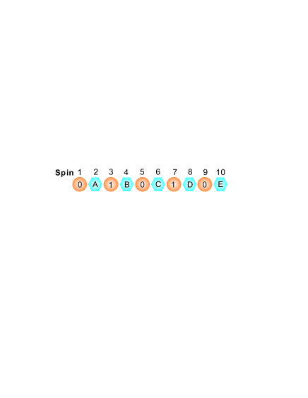
Figure 1: For the always-on $\sum\limits_{i=1}^{2n}J_{1}\sigma_{i}^{z}\sigma_{i+1}^{z}$ type inter-spin coupling, qubits will suffer continuous phase gates with their neighbors. We may only use the even spins (the hexagonal ones) to encode information while use the odd spins (the rounded ones) as blockade spin. When performing single qubit operation, the blockade spins are “frozen” in definite states $\left|0\right\rangle$ or $\left|1\right\rangle$ in order to negate influence of the perpetual Ising interaction.

When we perform quantum gates, the theoretical expected unitary evolution of the whole chain is $U=\exp(-itH_{Ideal})$ while the realistic evolution is $V=\exp[-it(H_{Ideal}+H_{L})]$. We could estimate the deviation $\left\|U-V\right\|$ in single and multi qubit operations, where for convenience we use the definition of spectral norm, that is, the norm of an operator $O$ is defined as the square root of the maximum eigenvalue of $O^{\dagger}O$. As shown in appendix. A, when we perform a certain quantum gate, the deviation induced by the omitted next-nearest-neighbor interaction is at least of the order $\left|\exp\{-iJ_{2}tn\}-1\right|$, $t$ being the required time for performing this gate. For $t$ very small, we could estimate the deviation speed:

$$\frac{d}{dt}\left\|U-V\right\|\backsim O(nJ_{2})$$ (5)

This result implies that, though $J_{2}$ is very small, deviation induced by $H_{L}$ could become very large because this deviation depends on the length of the chain. This deviation could increase with the chain become longer. Thus omitting the long-range interaction effect may restrict the scalability of previous schemes. Below we consider how to handle this problem by using proper encoding methods.

III
Using Encoding Schemes To suppress the influence of long-range interaction

Let us illustrate our idea intuitively. Following the previous section we start with a $1$-D spin-$1/2$ chain with tunable nearest-neighbor $XXZ$ interaction and next-nearest-neighbor Ising interaction. The Hamiltonian reads:

$$H_{M}=H_{S}+H_{I}+H_{L}$$ (6)

Where $H_{S}$, $H_{I}$, and $H_{L}$ are described by Eqs. 2-4. Here, we further set $B_{z}^{i}=0$ for any $i$ in the whole quantum information process, i. e. there is no $\sigma^{z}$ terms in $H_{S}$.

As sketched in Fig. 2, we encode one logical qubit by two physical spins, using the spin states $\left|01\right\rangle$ and $\left|10\right\rangle$ as logical $\left|0\right\rangle$ and $\left|1\right\rangle$. Thus the tunable $XY$ interaction between two spins plays the role of $\sigma^{x}$ rotation in the 2-D logical Hilbert space Wu2 .

Similar to the “blockade spin” methods used in ref. Bose1 , our intuitive idea is freezing two “blockade spins” between each two logical qubits to negate the influence of the nearest-neighbor and next-nearest-neighbor always-on Ising type interaction. As shown in Fig. 2: The hexagonal ones are spins used to encode information while the octagonal ones are used as blockade. We use the spins 3 and 4 as one logical qubit while spins 7 and 8 as another. When performing single qubit operations, we would make the blockade spins (spins 1, 2, 5, 6, 9, and 10) all “frozen” in state $\left|0\right\rangle$, thus the influence of permanent Ising type interaction on single logical qubit can be effectively negated: Since spin $3$-$4$ are in Hilbert subspace spanned by spin states $\left|01\right\rangle$ and $\left|10\right\rangle$, we simply calculate the influence of Ising type interactions on the logical qubit and get:

$$J_{1}(\sigma_{2}^{z}\sigma_{3}^{z}+\sigma_{4}^{z}\sigma_{5}^{z})+J_{2}(\sigma_{1}^{z}\sigma_{3}^{z}+\sigma_{2}^{z}\sigma_{4}^{z}+\sigma_{3}^{z}\sigma_{5}^{z}+\sigma_{4}^{z}\sigma_{6}^{z})=0$$ (7)

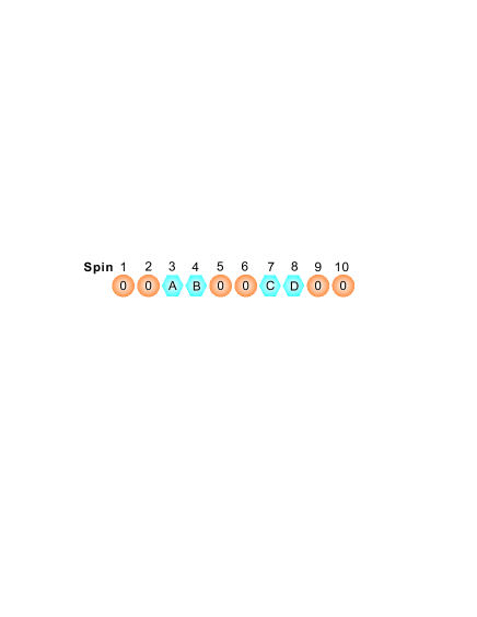
Figure 2: We use two spins to encode one logic qubit, that is, the two spins 3-4 as one qubit and spins 7-8 as another. Two “blockade spins” both in $\left|0\right\rangle$ state are placed between two logical qubits in order to negate the influence of next-nearest-neighbor interaction.

Now we show how to perform universal quantum gates, that is, the single qubit $\sigma^{x}$ rotations, the single qubit $\sigma^{z}$ rotations, and CPHASE gates between two qubits. As shown in Fig. 2, performing the single qubits $\sigma^{x}$ rotations on qubit encoded by spin 3 and 4 is easy by tuning $J_{3,4}$. We further note a trivial fact mentioned by ref. Zhou3 that the single qubit $\sigma^{z}$ rotation can be constructed by the CPHASE gate and single qubit $\sigma^{x}$ rotation. So the central problem becomes performing CPHASE gate between two logical qubits. Our main idea to achieve this goal is, by tuning the exchange interaction $J_{4,5}$ and $J_{6,7}$, we could perform a CPHASE gate between logical qubits encoded by spin 3-4 and spin 7-8, adding a phase on one of the four logical qubits states while remain the other three states unchanged.

We separate the spins 3, 4 and 5 as one party and spins 6, 7 and 8 as the other. We set $B_{x}^{i}=0$ for any i in the whole process of performing two qubit gate. Starting with the four possible initial states $\left\{\left|100\right\rangle,\left|010\right\rangle\right\}_{3,4,5}\bigotimes\left\{\left|010\right\rangle,\left|001\right\rangle\right\}_{6,7,8}$, initially we tune all the strength of nearest-neighbor $XY$ interaction to zero: $J_{i,i+1}=0$ for any i. Thus the the four possible logical qubits states have equal static energy and we define this static energy as energy zero point. As mentioned above, in performing two qubit gate, what we may tune is just $J_{4,5}$ and $J_{6,7}$, so we can reduce the Hamiltonian $H_{M}$ in Eq. 6 into a $9$-D Hilbert space

$$S=span\{\left\{\left|100\right\rangle,\left|010\right\rangle,\left|001\right\rangle\right\}_{3,4,5}\bigotimes\left\{\left|001\right\rangle,\left|010\right\rangle,\left|100\right\rangle\right\}_{6,7,8}\}$$ (8)

The whole Hamiltonian $H_{M}$ becomes a function of tunable $J_{4,5}$ and $J_{6,7}$: $H_{M}=H_{M}(J_{4,5},J_{6,7})$. Below we use the label $\left|abcdef\right\rangle$ to label the quantum states of the six spins from spin 3 to spin 8, the first $a$ for spin 3, the second $b$ for spin 4…… the last $f$ for spin 8. For example, $\left|100010\right\rangle$ labels the state in which the spin 3 and spin 7 are in state $\left|1\right\rangle$ while the spin 4, 5, 6 and 8 are in state $\left|0\right\rangle$.

Indeed, $S$ in Eq. 8 can be reduced to four Hilbert subspaces: The first one is a 1-D trivial subspace $S_{1}$ spanned by single state $\left|100001\right\rangle$. The second is 2-D

$$S_{2}=span\{\left\{\left|100\right\rangle\right\}_{3,4,5}\bigotimes\left\{\left|010\right\rangle,\left|100\right\rangle\right\}_{6,7,8}\}$$ (9)

Under basis $\left\{\left|100010\right\rangle,\left|100100\right\rangle\right\}$ Hamiltonian $H_{M}(J_{4,5},J_{6,7})$ can be reduced to:

$$H_{2}(J_{4,5},J_{6,7})=\left[\begin{array}[]{cc}0&2J_{6,7}\\ 2J_{6,7}&0\end{array}\right]$$ (10)

The third is similar to the second:

$$S_{3}=span\{\left\{\left|010\right\rangle,\left|001\right\rangle\right\}_{3,4,5}\bigotimes\left\{\left|001\right\rangle\right\}_{6,7,8}\}$$ (11)

Under basis $\left\{\left|010001\right\rangle,\left|001001\right\rangle\right\}$ the reduced Hamiltonian is

$$H_{3}(J_{4,5},J_{6,7})=\left[\begin{array}[]{cc}0&2J_{4,5}\\ 2J_{4,5}&0\end{array}\right]$$ (12)

The fourth is 4-D

$$S_{4}=\left\{\left|010\right\rangle,\left|001\right\rangle\right\}_{3,4,5}\bigotimes\left\{\left|010\right\rangle,\left|100\right\rangle\right\}_{6,7,8}$$ (13)

Under basis $\left\{\left|010010\right\rangle,\left|010100\right\rangle,\left|001010\right\rangle,\left|001100\right\rangle\right\}$ the reduced Hamiltonian is

$$H_{4}(J_{4,5},J_{6,7})=\left[\begin{array}[]{cccc}0&2J_{6,7}&2J_{4,5}&0\\ 2J_{6,7}&-4J_{2}&0&2J_{4,5}\\ 2J_{4,5}&0&-4J_{2}&2J_{6,7}\\ 0&2J_{4,5}&2J_{6,7}&-4J_{1}\end{array}\right]$$ (14)

The form of $H_{4}(J_{4,5},J_{6,7})$ is quite similar to the NMR type Hamiltonian: If we set $span\left\{\left|010\right\rangle,\left|001\right\rangle\right\}_{3,4,5}$ as the left “qubit” and $span\left\{\left|010\right\rangle,\left|100\right\rangle\right\}_{6,7,8}$ as the right, we could see that $J_{4,5}$ and $J_{6,7}$ play the role of tunable local $X$ operation for individual 2-D Hilbert space, and the perpetual Ising type interaction induce an untunable term of the type $a(\sigma_{L}^{z}+\sigma_{R}^{z})+b\sigma_{L}^{z}\sigma_{R}^{z}$ in the Hamiltonian. Unfortunately, techniques developed for NMR such as refocusing usually can not be employed in other systems (especially many solid state systems including quantum dot and superconducting circuits) because the assumption of fast, strong pulse can not be valid, so we choose an alternative way to perform CPHASE gate.

Starting with the four possible initial states with degenerate static energy, $\left\{\left|100\right\rangle,\left|010\right\rangle\right\}_{3,4,5}\bigotimes\left\{\left|010\right\rangle,\left|001\right\rangle\right\}_{6,7,8}$, in the first step we tune only $J_{4,5}$ while set $J_{6,7}=0$. The $XXZ$ interaction between spin 4 and 5 keeps states $\left|100001\right\rangle$ and $\left|100010\right\rangle$ unchanged.

In space $S_{3}$ taking Bloch sphere representation we see the transformation induced by $J_{4,5}$ is a rotation about $X$ axis. But in space $S_{4}$ the induced rotation is more complex. We note that since our initial state in $S_{4}$ is only $\left|010010\right\rangle$, the induced transformation in $S_{4}$ is finally reduced to a 2-D subspace $S_{4}^{{}^{\prime}}=span\{\left\{\left|010\right\rangle,\left|001\right\rangle\right\}_{3,4,5}\bigotimes\left\{\left|010\right\rangle\right\}_{6,7,8}\}$. Under basis $\left\{\left|010010\right\rangle,\left|001010\right\rangle\right\}$ the reduced Hamiltonian is

$$H_{4}^{{}^{\prime}}(J_{4,5},0)=\left[\begin{array}[]{cc}0&2J_{4,5}\\ 2J_{4,5}&-4J_{2}\end{array}\right]$$ (15)

The induced transformation is a rotation about an axis on $X-Z$ plane because the static energy of $\left|010010\right\rangle\allowbreak$ and $\left|001010\right\rangle$ are slightly different due to the long-range interaction $H_{L}$.

So in $S_{4}^{{}^{\prime}}$, with tunable $J_{4,5}$ acting as $\sigma^{x}$-operation, we can perform a transformation $\exp\left\{-i\pi\sigma^{x}/2\right\}$, which is exactly a $\pi$ rotation around the $X$-axis in Bloch sphere representation. We assume that the maximum value of $J_{4,5}$ we could tune to is $X_{1}/2$. We set parameter $\theta$ and $X_{2\text{ }}$as $\cos\theta=\frac{X_{1}}{\sqrt{X_{1}^{2}+\left(2J_{2}\right)^{2}}}$, $\sin\theta=\frac{2J_{2}}{\sqrt{X_{1}^{2}+\left(2J_{2}\right)^{2}}}$, $\cos 2\theta=\frac{X_{2}}{\sqrt{X_{2}^{2}+\left(2J_{2}\right)^{2}}}$, and $\sin 2\theta=\frac{2J_{2}}{\sqrt{X_{2}^{2}+\left(2J_{2}\right)^{2}}}$. Then we define rotation (we set $\hbar=1$)

$$R(X)=\exp\left[iH_{4}^{{}^{\prime}}(X,0)\pi/2\sqrt{X^{2}+\left(2J_{2}\right)^{2}}\right]$$ (16)

Thus we have

$$R(X_{1})=i\left[\begin{array}[]{cc}\sin\theta&\cos\theta\\ \cos\theta&-\sin\theta\end{array}\right]$$ (17)

$$R(X_{2})=i\left[\begin{array}[]{cc}\sin 2\theta&\cos 2\theta\\ \cos 2\theta&-\sin 2\theta\end{array}\right]$$ (18)

And the combined rotation in subspace $S_{4}^{{}^{\prime}}$ is what we want:

$$R(X_{1})R(X_{2})R(X_{1})=\exp\left\{-i\pi\sigma^{x}/2\right\}$$ (19)

These above tuning of $J_{4,5}$ at last form a unitary transformation $U_{1}$ in the $9$-D space $S$: It is nontrivial only in space $S_{3}$ and $S_{4}^{{}^{\prime}}$: $\left|100001\right\rangle$ and $\left|100010\right\rangle$ remain unchanged; $\left|010010\right\rangle$ is transformed exactly into $\left|001010\right\rangle$; $\left|010001\right\rangle$ is transformed into superposition of $\left|010001\right\rangle$ and $\left|001001\right\rangle$. As shown in Eqs. 16–19, the required time for this step is $T_{1}=\pi/\sqrt{X_{1}^{2}+\left(2J_{2}\right)^{2}}+\pi/2\sqrt{X_{2}^{2}+\left(2J_{2}\right)^{2}}$. We could see that $T_{1}$ mainly depends the maximal $XY$ interaction strength we could have. We further note an important fact that if we re-perform the tuning of $J_{4,5}$ with inverse strength, i.e. $X_{1}$ to $-X_{1}$, $X_{2}$ to $-X_{2}$, we can get the inverse operation of $U_{1}$ in $S$.

In the second step we tune $J_{4,5}$ to zero but come to control $J_{6,7}$. Quite similar to the previous step, this exchange interaction keeps states in $S_{1}$ and $S_{3}$ unchanged while induce transformations in $S_{2}$ and $S_{4}$. In $S_{2}$ under Bloch sphere representation the induced transformation is a rotation about $X$ axis, while in subspace $S_{4}$, since the initial state $\left|010010\right\rangle$ is exactly transformed into state $\left|001010\right\rangle$ by the first step, the induced transformation by $J_{6,7}$ in $S_{4}$ is restricted to a 2-D subspace $S_{4}^{{}^{\prime\prime}}=\left\{\left|001\right\rangle\right\}_{3,4,5}\bigotimes\left\{\left|010\right\rangle,\left|100\right\rangle\right\}_{6,7,8}$. Under basis $\left\{\left|001010\right\rangle,\left|001100\right\rangle\right\}$ the reduced Hamiltonian is

$$H_{4}^{{}^{\prime\prime}}(0,J_{6,7})=\left[\begin{array}[]{cc}-4J_{2}&2J_{6,7}\\ 2J_{6,7}&-4J_{1}\end{array}\right]$$ (20)

The form of $H_{4}^{{}^{\prime\prime}}(0,J_{6,7})$ is quite similar to that of the previous $H_{4}^{{}^{\prime}}(J_{4,5},0)$, so we can perform another unitary transformation $U_{2}$ just similar to the first step which implement a $\pi$ rotation around the $X$-axis in space $S_{4}^{{}^{"}}$, transforming state $\left|001010\right\rangle$ to $\left|001100\right\rangle$.

After the above two steps, we review the intermediate states we get: $\left|100001\right\rangle$ remain unchanged; $\left|100010\right\rangle$ is changed into the superposition of $\left|100010\right\rangle$ and $\left|100100\right\rangle$; $\left|010001\right\rangle$ is changed into the superposition of $\left|010001\right\rangle$ and $\left|001001\right\rangle$; $\left|010010\right\rangle$ is changed into $\left|001100\right\rangle$. The previous three intermediate states are degenerate under Hamiltonian $H_{M}\left(0,0\right)$ but the last state has nonzero static energy $-4J_{1}$. Therefore, in the third step we tune off all exchange coupling for a time interval $\tau$. In this period the state $\left|001100\right\rangle$ experience an additional phase $\varphi$ due to its non-zero static energy. In the last step we can perform the inverse operation of $U_{2}$ and $U_{1}$ to transform the four intermediate states back to the initial four states.

After all the above operations we have performed a CPHASE gate $U\left(\varphi\right)$ between two qubits, adding a controllable phase $\varphi$ on the state $\left|010010\right\rangle$ while remaining other states unchanged. As we mentioned before, we use spin states $\left|01\right\rangle$ for spin 3-4 and spin 7-8 as logical $\left|0\right\rangle$ and $\left|10\right\rangle$ as logical $\left|1\right\rangle$, in this 4-D representation the gate $U\left(\varphi\right)$ we obtain is

$$\left[\begin{array}[]{cccc}1&0&0&0\\ 0&e^{i\varphi}&0&0\\ 0&0&1&0\\ 0&0&0&1\end{array}\right]$$ (21)

After implementation of the CPHASE gate $U$, we note that Zhou3 $\left(\sigma_{2}^{x}\ast U(2\varphi)\right)^{2}=e^{i\varphi}e^{i\sigma_{1}^{z}\varphi}$, thus with the single qubit $\sigma^{x}$ rotation of the second qubit and CPHASE gate between the first and the second qubit, the single qubit $\sigma^{z}$ rotation of the first qubit is obtained.

In summary of this section, we have demonstrated all the required universal gates for QC. In this scheme, by using appropriate encoding method, influence of the next-nearest-neighbor interaction is effectively ruled out, thus the precision of quantum gates updated. Besides, the speed of the CPHASE gate mainly depends on the strength of nearest-neighbor exchange interaction, it is not restricted by the small value of $J_{2}$. The quantum information speed of this scheme is in the same level with that of previous schemes in which the next-nearest-neighbor interaction was neglected.

IV A potential physical realization: Josephson Junction Charge Qubit

Now we consider the application of our scheme to realistic systems. We consider the long-range interaction in Josephson charge qubit system as an example. The typical Josephson-junction charge qubit is shown in Fig. 3 Schon1 : It consists of a small superconducting island with $n$ excess Cooper pairs, connected by a tunnel junction with capacitance $C_{J}$ and Josephson coupling energy $E_{J}$ to a superconducting electrode. A control gate voltage $V_{g}$ is coupled to the system via the gate capacitor $C_{g}$. The Hamiltonian of the Cooper pairs box (CPB) is

$$H_{Josephson}=E_{c}(n-n_{g})^{2}+E_{J}\cos\Phi$$ (22)

where $E_{c}=(2e)^{2}/2\left(C_{g}+C_{J}\right)$ is the charge energy, $n_{g}=C_{g}V_{g}/2$ is the gate charge, and $\Phi$ is the conjugate variable to $n$. When $E_{c}\gg E_{J}$, by choosing $n_{g}$ close to the degeneracy point $n_{g}=1/2$, only the states with $0$ and $1$ Cooper pairs play a role while all other charge states in much higher energy level can be ignored. In this case the CPB can be reduced to an effective two-state quantum system. A further step is replacing the single Josephson junction by two identical junctions in a loop configuration in order to gain tunable tunnelling amplitude Schon2 . By making replacement $n=\left(1+\sigma^{z}\right)/2$, the effective Hamiltonian can be written in the spin-$1/2$ notation as

$$H_{Josephson}=-B_{z}\sigma^{z}-B_{x}\sigma^{x}$$ (23)

where the state with $0$ Cooper pairs corresponds to the spin state $\left|\downarrow\right\rangle$ and $1$ Cooper pairs to $\left|\uparrow\right\rangle$. $B_{z}$ and $B_{x}$ are the effective magnetic fields which are controlled by the biased gate voltage and frustrated magnetic flux.

Figure 3: A Josephson charge qubit formed by a superconducting single-charge box and a tunnel junction.The single Josephson junction is replaced by a flux-frustrated SQUID so that the effective Josephson coupling is tunable.

For coupling two CPBs, the direct capacitance coupling Nakamura2 Nakamura3 is most intrinsic, but its drawback is also obvious, that is, the coupling strength induced by connective capacitances is untunable. For a system consist of $M$ CPBs coupled with each other by capacitances, the static charge energy can be written as Mooij2 Berman

$$H_{C}=\frac{\left(2e\right)^{2}}{2}\overrightarrow{n}C^{-1}\overrightarrow{n}^{\dagger}$$ (24)

where $\overrightarrow{n}=(n_{1}-n_{g1},n_{2}-n_{g2},n_{3}-n_{g3},......n_{M}-n_{gM})$ is the charge number vector of the $M$ CPBs, and $C$ is the capacitance matrix of the system whose diagonal term $C_{i,i}$ equals to the sum of capacitance around the $ith$ CPB, and non diagonal term $C_{i,j}$ corresponds to the connective capacitance between CPB $i$ and $j$.

A schematic plot of an array of $N$ capacitively coupled CPBs is shown in Fig. 4. The CPBs have Josephson energies $E_{Ji}$ and capacitances $C_{Ji}$. Each CPB is connected to the control gate voltages $V_{gi}$ via a gate capacitance $C_{gi}$. The $i$th intermediate CPB is connected to its neighboring $\left(i\pm 1\right)$th CPBs via the connective capacitors $C_{ci,i\pm 1}$. We assume that all CPBs are identical with the same capacitances: $C_{gi}=C_{g}$, $C_{Ji}=C_{J}$, and all the coupling capacitance $C_{ci,i+1}$ are equal to $C_{c}$. So we have a tridiagonal capacitance matrix for this system. For the intermediate qubits of the array,

$$C_{i,j}=C_{0}[\delta_{i,j}(1+2\epsilon)-\delta_{i,j\pm 1}\epsilon],1<i,j<N$$ (25)

where $C_{0}=C_{g}+C_{J}$ and $\epsilon=C_{c}/C_{0}$. For qubits on the edge of the array a small correction is needed: $C_{1,1}=C_{N,N}=C_{0}(1+\epsilon)$ while $C_{1,2}=C_{N-1,N}=-C_{0}\epsilon$.

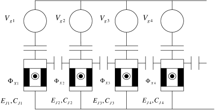
Figure 4: A schematic illustration of array of capacitively coupled CPBs.

Since $C$ is a tridiagonal matrix, $C^{-1}$ has nonzero matrix elements on the second, third and other diagonals which characterize the capacitance induced Coulomb interaction between different CPBs. If $\epsilon\ll 1$, the off-diagonal elements of $C^{-1}$ decay exponentially as $C_{i,j}^{-1}\sim C_{i,i}^{-1}\epsilon^{\left|i-j\right|}$. So the influence of the long-range interaction can be reduced by taking the coupling capacitances $C_{c}$ much smaller than the on-site capacitances $C_{0}$. Again by making replacement $n_{i}=\left(1+\sigma_{i}^{z}\right)/2$, we get that the interaction term $C_{i,j}^{-1}(n_{i}-n_{gi})(n_{j}-n_{gj})$ provides always-on Ising type interaction between CPB $i$ and $j$.

If we go further, replacing the coupling capacitance by SQUID, we can have tunable $XY$ type exchange interaction between neighboring qubit besides perpetual Ising type interaction (Fig. 5) Siewert1 Siewert2 Sun1 . Due to flux quantization the phase across the coupling SQUID is $\Phi_{1}-\Phi_{2}+\alpha$, $\alpha$ being a constant controlled by the frustrated flux. If we tune $\alpha$ to zero, the coupling term $\cos(\Phi_{1}-\Phi_{2})$ thus induce $XY$ type exchange interaction $\sigma_{1}^{x}\sigma_{2}^{x}+\sigma_{1}^{y}\sigma_{2}^{y}$.

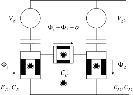
Figure 5: A schematic plot of two CPBs coupled by a SQUID.

Thus we can see the correspondence between the theoretical Hamiltonian in Eq. 6 and the realistic physical system: the tunable SQUIDs of single qubits induce tunable $\sigma^{x}$ terms in the single qubit part of Hamiltonian; all the bias voltages are biased on the degeneracy point $V_{gi}=1/2$ in order to prevent the qubits from the $1/f$ noise effect Vion , implying that there is no $\sigma^{z}$ term in the single qubit part of Hamiltonian; the exponentially decay capacitance coupling corresponds to the nearest Ising interaction part in $H_{I}$ and the next-nearest-neighbor Ising interaction part $H_{L}$, while the tunable SQUID coupling corresponds to the tunable $XY$ interaction part in $H_{I}$. We also see that the required performances in the above scheme just correspond to tuning external magnetic field frustrated in the SQUID loops.

By taking $\epsilon\ll 1$ the effect of the long-range interaction in Josephson charge qubit array system can be reduced but can never be negated. Moreover, the speed of two qubits operation depends on $\epsilon$, decreasing the value of $\epsilon$ would slow the speed of two qubits gate. Besides, making $\epsilon$ smaller and smaller may be highly challenging in experimental realization. So we may choose an alternative way to handle the problem of always-on non-nearest-neighbor coupling. The main idea is that, based on the decay property of the long-range interaction, we can take some lower order terms of long-range interaction into account while taking the higher order terms as random noise. Thus we may use the encoding schemes discussed in Sec. III to negate the influence of the few lowest order couplings.

Schemes of using capacitively coupled Josephson array to perform QC have been proposed Berman Averin . Our scheme offer an alternative idea to handle the long-range interaction problem. The only parameter required to tune is the flux frustrated in SQUID loops, while the gate voltages are frozen on the degeneracy point, which prevents qubits from severe dephasing.

It should be noted that, in our scheme although the next-nearest-neighbor interaction effect is entirely negated, the higher order long-range couplings still work. A natural generalization is using $3$ spins as one “blockade” to negate the influence of the third order long-range interaction (first order being the nearest-neighbor coupling while second order being the next-nearest-neighbor coupling), or even $m$ spins as one “blockade” to negate the influence of the $m$th order long-range interaction. Following analysis similar to the estimation in appendix. A, we could conclude that, if we have negated the influence of the $m$th order interaction, the speed of deviation from ideal unitary evolution will be $O(nJ_{m+1})$, $J_{m+1}$ being the characteristic interaction strength of the $(m+1)$th order coupling. In $1$-D Josephson charge qubit array system the strength of the long-range interaction have exponentially decay property, this means that, for a certain $n$, we could always make $nJ_{m+1}$ small enough. So we could apply the generalization of our QC scheme to this physical system to suppress the speed of deviation induced by long-range interaction into some tolerable domain. Another potential extension is generalizing the nearest-neighbor coupling in our scheme from $XXZ$ type to various other types including $XY$ type and Heisenberg type. We could also translate our idea of handing long-range interaction in this paper to other implementations.

V conclusion

In conclusion, in this paper we have studied the non-nearest-neighbor interaction effect in $1$-D spin-$1/2$ chain model. We prove that the quantum gate deviation induced by the long-range interaction may challenge the scalability of quantum computing. We further propose a QC scheme in order to suppress influence of long-range interaction. In this scheme, using appropriate encoding method, we effectively neutralize influence of the next-nearest-neighbor interaction, thus the precision of quantum gates updated. The quantum information speed of this scheme is in the same level with that of previous schemes in which the long-range interaction strength was ignored. We also discuss the feasibility of the scheme in $1$-D Josephson charge qubit array system. This scheme may offer improvement in dealing with systematic errors in scalable quantum computing.

Appendix A Estimation of deviation induced by long-range interaction

Let us follow schemes developed in ref. Bose1 . As shown in Fig. 1: In the spin-$1/2$ chain, only the even spins (the hexagonal ones) are chosen as qubits while the odd spins (the rounded ones) are used as “blockade”.

When we perform quantum gates following schemes developed in ref. Bose1 , the theoretical expected unitary evolution is $U=\exp(-itH_{Ideal})$ while the realistic evolution is $V=\exp[-it(H_{Ideal}+H_{R})]$, We could estimate the deviation $\left\|U-V\right\|$ in single and multi qubit operations:

(1) Idle. When the whole chain is in idle status, the single qubit part $H_{S}$ and the exchange interaction term in $H_{I}$ are all tuned off, the $n+1$ odd spins used as “blockade spins” are “frozen” in definite states $\left|0\right\rangle$ or $\left|1\right\rangle$. Since the permanent nearest-neighbor and next-nearest-neighbor Ising type interaction do not transfer energy, we could reduce our discussion in a $2^{n}$-D Hilbert space $H$ which is direct product of all the $n$ qubits. The expected evolution is $U_{Idle}=I$. But the realistic evolution is

$$V_{Idle}=\exp\{-iJ_{2}t[-n+\sum_{i=1}^{n-1}\sigma_{2i}^{z}\sigma_{2i+2}^{z}]\}$$ (26)

$\sigma_{j}^{x}$, $\sigma_{j}^{y}$, and $\sigma_{j}^{z}$ being Pauli operators of the $j$th spin. Eigenvalues of $V_{Idle}$ varys from $\exp\{iJ_{2}t\}$ to $\exp\{-iJ_{2}t[-2n+1]\}$. $\exp\{iJ_{2}t\}$ corresponds to states that the $n$ qubits are all in state $\left|0\right\rangle$ or all in state $\left|1\right\rangle$, while $\exp\{-iJ_{2}t[-2n+1]\}$ corresponds to states that for any $i$ the $2i$th spin and the $2(i+1)$th spin are in opposite states. We could choose a proper energy zero point for realistic evolution process, this means we could add a proper phase factor on $V_{Idle}:$ $V_{Idle}\rightarrow e^{i\varphi}V_{Idle}.$ But no matter how we choose the energy zero point, we could prove that, for any $\varphi$, either

$$\left|e^{i\varphi}\exp\{-iJ_{2}t[-2n+1]\}-1\right|\geq\left|\exp\{-iJ_{2}t[n-1]\}-1\right|$$ (27)

or

$$\left|e^{i\varphi}\exp\{iJ_{2}t\}-1\right|\geq\left|\exp\{-iJ_{2}t[n-1]\}-1\right|$$ (28)

is valid. So we could give an estimation of deviation for idle status:

$$\left\|U-V\right\|_{Idle}\geq\left|\exp\{-iJ_{2}t[n-1]\}-1\right|$$ (29)

(2) Performing $\sigma^{z}$ rotations. When performing $\sigma^{z}$ rotations on the $2i$th spin, parts for other spins in $H_{S}$ and all $J_{i,i+1}$ for any $i$ are tuned off, the $n+1$ odd spins used as “blockade spins” are “frozen” in definite states $\left|0\right\rangle$ or $\left|1\right\rangle$ as shown in Fig. 1. We could estimate the deviation $\left\|U_{z}-V_{z}\right\|$ in a $2^{n-1}$-D Hilbert space $H_{z}$. $H_{z}$ is defined as below: $H_{z}$ is a subspace of $H$. It is the direct product of all the $n$ qubits except the $i$th, and for any state in $H_{z}$, the $i$th qubit is in state $\left|0\right\rangle$. The expected evolution in $H_{z}$ is $U_{z}=\exp[-itB_{z}^{2i}]$. But the realistic evolution is

$$V_{z}=\exp\{-it[B_{z}^{2i}-nJ_{2}+J_{2}\sigma_{2i-2}^{z}+J_{2}\sigma_{2i+2}^{z}+J_{2}\sum_{k=1,k\neq i-1,k\neq i}^{n-1}\sigma_{2k}^{z}\sigma_{2k+2}^{z}]\}$$ (30)

Thus the estimation of deviation in $H_{z}$ is quite similar to previous idle status:

$$\left\|U-V\right\|_{z}^{H_{z}}\geq\left|\exp\{-iJ_{2}t[n-1]\}-1\right|$$

We note that the norm of operator $U-V$ in the whole space $H$ could not be smaller than the norm of operator $U-V$ reduced in a subspace $H_{z}$ of $H$. So we give an estimation of deviation for performing $\sigma^{z}$ gate:

$$\left\|U-V\right\|_{z}\geq\left|\exp\{-iJ_{2}t[n-1]\}-1\right|$$ (31)

(3) Performing $\sigma^{x}$ rotations. Discussion of performing $\sigma^{x}$ rotations on the $i$th qubit is similar to previous discussion of performing $\sigma^{z}$ rotations on the $i$th qubit. Similarly we could define a subspace $H_{x}$ of $H$: It is the direct product of qubits except the $(i-1)$th, $i$th, and $(i+1)$th qubits, and for any state in $H_{x}$, the $(i-1)$th qubit is in state $\left|0\right\rangle,$ the ith qubit is in state $(\left|0\right\rangle+\left|1\right\rangle)/\sqrt{2},$ and the $(i+1)$th qubit is in state $\left|1\right\rangle.$ So we have $J_{2}\sigma_{2i-2}^{z}\sigma_{2i}^{z}+J_{2}\sigma_{2i}^{z}\sigma_{2i+2}^{z}=0.$ The expected evolution in this subspace is $U_{x}=\exp[-itB_{x}^{2i}]$, while the realistic evolution is

$$V_{x}=\exp\{-it[B_{x}^{2i}-nJ_{2}+J_{2}\sigma_{2(i-2)}^{z}-J_{2}\sigma_{2(i+2)}^{z}+J_{2}(\sum_{k=1}^{i-2}+\sum_{k=i+1}^{n-1})\sigma_{2i}^{z}\sigma_{2i+2}^{z}]\}$$ (32)

Eq. 32 is similar to Eq. 30. We give the estimation:

$$\left\|U-V\right\|_{x}\geq\left|\exp\{-iJ_{2}t[n-3]\}-1\right|$$ (33)

(4) Performing inter-qubit gate. Inter-qubit gate between the $i$th qubit and the $(i+1)$th qubit is achieved by tuning the inter-spin exchange interaction strength $J_{2i,2i+1}$ and $J_{2i+1,2i+2}$ while other exchange interaction terms are all tuned off. Suppose in idle status the blockade spin $2i$ is in state $\left|0\right\rangle$, we could estimate the deviation in a $2^{n-2}$ Hilbert space $H_{int}.$ $H_{int}$ is defined as follow: $H_{int}$ is a subspace of $H$; It is the direct product of all qubits except the $i$th and $(i+1)$th qubits. For any state in $H_{int}$, the $i$th and the $(i+1)$th qubits are both in state $\left|0\right\rangle$. Obviously the ideal expected evolution in this space is $I$, but the realistic evolution is

$$V_{int}=\exp\{-it[-(n-1)J_{2}-J_{2}\sigma_{2(i-1)}^{z}-J_{2}\sigma_{2(i+2)}^{z}+J_{2}(\sum_{k=1}^{i-2}+\sum_{k=i+2}^{n-1})\sigma_{2k}^{z}\sigma_{2k+2}^{z}]\}$$ (34)

Quite similar to previous estimations we give:

$$\left\|U-V\right\|_{int}\geq\left|\exp\{-iJ_{2}t[n-2]\}-1\right|$$ (35)

References

- (1) X. X. Zhou, Z. W. Zhou, G. C. Guo, and M. J. Feldman, Phys. Rev. Lett. 89, 197903 (2002).
- (2) Z. W. Zhou, B. Yu, X. X. Zhou, M. J. Feldman, and G. C. Guo, Phys. Rev. Lett. 93, 010501 (2004).
- (3) S. C. Benjamin and S. Bose, Phys. Rev. Lett. 90, 247901 (2003).
- (4) F. Troiani, M. Affronte, S. Carretta, P. Santini, and G. Amoretti, Phys. Rev. Lett. 94, 190501 (2004).
- (5) B. W. Lovett, quant-ph/0508192 (2005).
- (6) L. A. Wu and D. A. Lidar, Phys. Rev. A. 65, 042318 (2002).
- (7) A. Shnirman, G. Schon, and Z. Hermon, Phys. Rev. Lett. 79, 2371 (1997).
- (8) Y. Makhlin, G. Schon, and A. Shnirman, Nature (London) 398, 305 (1999).
- (9) Y. A. Pashkin, T. Yamamoto, O. Astafiev, Y. Nakamura, D. V. Averin and J. S. Tsai, Nature (London) 421, 823 (2003).
- (10) T. Yamamoto, Y. A. Pashkin, O. Astafiev, Y. Nakamura and J. S. Tsai, Nature (London) 425, 941 (2003).
- (11) T. P. Orlando, J. E. Mooij, L. Tian, C. H. van der Wal, L. S. Levitov, S. Lloyd, and J. J. Mazo, Phys. Rev. B. 60, 15398 (1999).
- (12) G. P. Berman, A. R. Bishop, D. I. Kamenev, A. Trombettoni, Phys. Rev. B. 71, 014523 (2005).
- (13) J. Siewert, R. Fazio, G. M. Palma, and E. Sciacca, J. Low Temp. Phys. 118, 795 (2000).
- (14) J. Siewert and R. Fazio, Phys. Rev. Lett. 87, 257905 (2001).
- (15) Y. D. Wang, Z. D. Wang, and C. P. Sun, quant-ph/0506144 (2005).
- (16) D. V. Averin, Solid State Commun. 105, 659 (1998).
- (17) X. X. Zhou, M. Wulf, Z. W. Zhou, G. C. Guo, and M. J. Feldman, Phys. Rev. A. 69, 030301(R) (2004).
- (18) D. Vion, A. Aassime, A. Cottet, P. Joyez, H. Pothier, C. Urbina, D. Esteve, and M. H. Devoret, Science 296, 886 (2002).