Wigner Function Evolution of Quantum States in Presence of Self-Kerr Interaction

Abstract

A Fokker-Planck equation for the Wigner function evolution in a noisy Kerr medium ($\chi^{(3)}$ non-linearity) is presented. We numerically solved this equation taking a coherent state as an initial condition. The dissipation effects are discussed. We provide examples of quantum interference, sub-Planck phase space structures, and Gaussian versus non-Gaussian dynamical evolution of the state. The results also apply to the description of a nanomechanical resonator with an intrinsic Duffing nonlinearity.

I Introduction

Nonlinear interaction of light in a medium provides a very useful framework to study various nonclassical properties of quantum states of radiation. These nonclassical properties are usually associated with quantum interference and entanglement. The phase space Wigner distribution function description of quantum states of light is a powerful tool to investigate such nonclassical effects. With the help of the Wigner function one can simply visualize quantum interference. For example, a signature of quantum interference is exhibited in the Wigner function by the non-positive values and sub-Planck structures Ludmila . The non-positive Wigner function is a witness of a nonclassicality and monitors a decoherence process of a quantum state, e.g. a photon-added coherent state in the photon-loss channel Shang , photon-subtracted squeezed state Agarwal , Gaussian quadrature-entangled single photon subtracted light pulse Grangier2007 , two-photon Fock state Grangier2006 , odd photon number states superposition Polzik and coherent states superpositions Jeong . The Wigner function has also been used for computing numerically the quantum-mechanical corrections to the classical dynamics of a nanomechanical resonator (its characteristic pattern, the interference fringes and negative values, served as a signature for a classical to quantum domain transition) Katz ; it has been applied in the model of the dynamics of a nanoscale semiconductor laser Weetman , to list only a few examples of its applications.

The Kerr medium provides one of the simplest nonlinearity for which there exists a simple analytic Wigner function Wigner expression. The highly $\chi^{(3)}$ nonlinear systems generated a lot of interest recently due to their applications e.g. to nondemolition measurements Imoto , quantum computing architectures Turchette , single particle detectors Mohapatra . The well known example of such a medium is an optical fiber. However, the nonlinearity is small in fibers and is often accompanied by other unwanted effects. Enhanced Kerr nonlinearity was studied in terms of electromagnetically induced transparency Imamoglu and was observed in Bose Einstein condensates Hau and cold atoms Kang . Recent proposals predict obtaining enormous Kerr nonlinearity using the Purcell effect Bermel , Rydberg atoms Mohapatra , and interaction of a cavity mode with atoms Brandao . The first and last method is predicted to obtain the nonlinearity of nine orders of magnitude higher than natural self-Kerr interactions with negligible losses. The significant nonlinearity has also been observed for nanomechanical resonators Kozinsky .

Most of the investigations of the Wigner function of light have been made for steady state situations. The simplicity of the Kerr medium will allow to study the full time-dependent Wigner function dynamics with or without a quantum noise.

In this paper we present a Fokker-Planck equation which determines the time evolution of the Wigner function in a noisy $\chi^{(3)}$ medium. We solve this equation numerically assuming a coherent state as an initial condition. We discuss first an ideal and then a dissipative Kerr medium. The results obtained for the ideal case reveal the quantum nature of the state under evolution. The coherent state, known as the most classical among all the pure states, becomes a non-Gaussian squeezed state after some time of interaction with the medium. For some specific times it becomes a finite superposition of other coherent states. An interference pattern with the negative values is clearly visible on the plots of its Wigner function. Due to the small value of the $\chi^{(3)}$ nonlinearity and losses in optical fibers such phenomena have never been observed for light; neither for any other system. However, it turns out that not all quantum effects are washed out due to the decoherence. The Fokker-Planck equation allows for a similar state evolution analysis for any other input state.

The paper is organized as follows: in section II the Fokker-Planck equation for the Wigner function evolution in a $\chi^{(3)}$ medium is derived from the Master equation obtained for a single mode of light density operator. The equation is displayed in a polar coordinates. The decoherence effects: losses and thermal noise are included. The initial and boundary conditions for the Wigner function are set. In section III the numerical results of the Wigner function evolution in a nondissipative $\chi^{(3)}$ medium are introduced and discussed. These results are obtained using three independent methods: computing the Fokker-Planck equation and the other two equations determining the Wigner function directly, which are obtained from its definition. Correspondence between the Wigner function negative values and zeros of the Q-function is noted. In section IV the influence of the decoherence process on quantum effects such as the interference pattern and the negative values of the Wigner function is analyzed. The technical limitations on the use of the Fokker-Planck equation are discussed. The Wigner function sub-Planck structure is shown in section V. In section VI the numerical methods used in sections III and IV are compared and discussed. Finally some conclusions are presented.

II The Fokker-Planck Equation for a Self-Kerr Interaction

The interaction Hamiltonian for a totally degenerate four-wave mixing process, e.g. in an optical fiber, is of second-order in creation $a^{\dagger}$ and annihilation $a$ light operators

$$H=\hbar\frac{\kappa}{2}\,a^{\dagger}a^{\dagger}a\,a,$$ (1)

where $\kappa$ is a nonlinear constant proportional to $\chi^{(3)}$ Tanas . Please note that similar Hamiltonian describes a single nanomechanical resonator with $a^{\dagger}$ and $a$ being raising and lowering operators related to its position and momentum operators, and $\kappa$ proportional to the Duffing nonlinearity Woolley .

In a general case, including damping and thermal noise in the medium, a one-mode density operator evolution, both for light and for a nanomechanical resonator, is determined by the Master equation Walls

$$\partial_{t}\rho(\tau) = -\frac{i}{\hbar}[H,\rho(\tau)]+\frac{\Gamma}{2}\left([a\rho(\tau),a^{\dagger}]+[a,\rho(\tau)a^{\dagger}]\right)$$ (2)

$$+ \Gamma N[[a,\rho(\tau)],a^{\dagger}],$$

where $\tau=-\kappa t$ is a unitless evolution parameter, $t$ is the interaction time, $\Gamma$ is a damping constant, $N=1/\{\exp\left(\frac{\hbar\omega}{kT}\right)-1\}$ is a mean number of photons in a thermal reservoir.

The solutions of the above equation are well known Tanas ; Milburn1986 ; Milburn1989 ; Perinova1990 but since it is an operator-valued equation, they are inappropriate for computer simulations. A Fokker-Planck type evolution equation for the Wigner function can be easily obtained from equation (2) using the standard quantum optics phase space methods Gardiner . Since every density operator determines its Wigner function uniquely, the knowledge of its evolution is equivalent to the full knowledge of the density operator dynamics.

The dynamics of the Wigner function in a dissipative medium with a self-Kerr interaction is governed by the Fokker-Planck equation, which takes the following form in the polar coordinates $\gamma=re^{i\varphi}$

$$\partial_{\tau}W(\tau,r,\varphi) = \left\{(r^{2}-1)\partial_{\varphi}-\frac{1}{16}\left(\frac{1}{r}\partial_{r}\partial_{\varphi}+\partial^{2}_{r}\partial_{\varphi}+\frac{1}{r^{2}}\partial^{3}_{\varphi}\right)\right.$$ (3)

$$+ \left.\xi+\frac{\xi}{2}\left(r+\frac{1}{2}\left(\frac{1}{2}+N\right)\frac{1}{r}\right)\partial_{r}\right.$$

$$+ \left.\frac{\xi}{4}\left(\frac{1}{2}+N\right)\left(\partial^{2}_{r}+\frac{1}{r^{2}}\partial^{2}_{\varphi}\right)\right\}W(\tau,r,\varphi),$$

where $\gamma$ is a point in a phase space, $\xi=\Gamma/\kappa$.

This is a third-order nonlinear differential equation. We compute this equation for the following initial and boundary conditions. The evolution starts with a coherent state $|\alpha\rangle$ described by a Wigner function $W(0,\gamma)=\frac{2}{\pi}e^{-2|\alpha-\gamma|^{2}}$. The Wigner function tends to zero in the infinity $\lim_{r\to\infty}W(\tau,r,\varphi)=0$. Since some of the coefficients in equation (3) are singular for $\gamma=0$, we take $W(\tau,0,0)=\frac{2}{\pi}e^{-2|\alpha|^{2}e^{-\tau\xi}}$, which was derived from the Master equation.

III The nonlinear part of evolution

For $\xi=0$ and $N=0$ the Fokker-Planck equation (3) reduces to its first line and describes the evolution in an ideal Kerr medium.

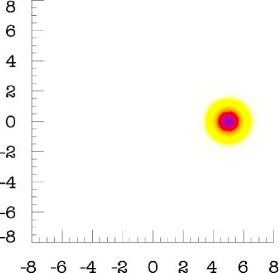
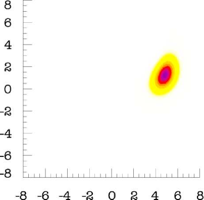
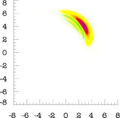
Figure 1: (Color online) The Wigner function for $\alpha=5$ and $\tau=0$ is a Gaussian function for the coherent state – the left figure. Due to the fact that the evolution in an ideal $\chi^{(3)}$ medium is periodic, we achieve the same shape of the Wigner function for $\tau=2\pi$. The distribution is an ellipse and the state becomes squeezed beginning from $\tau=0.01$ – the middle figure. The negative values of the function start to appear for $\tau=0.04$ – the right figure.

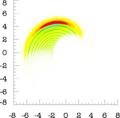
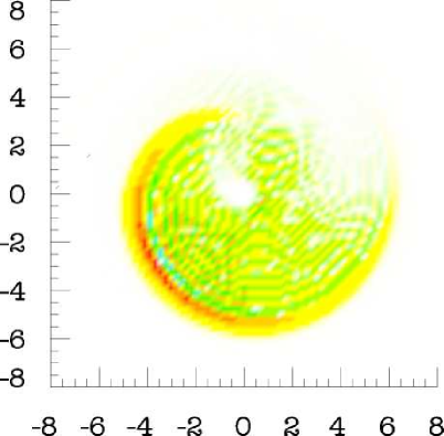
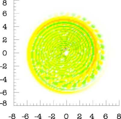
Figure 2: (Color online) Further steps of Wigner function evolution obtained also for $\alpha=5$ and $\tau=0.08$ – the left figure, $\tau=0.16$ – the middle figure and $\tau=0.3$ – the right figure. An interference pattern arises in the form of a “tail” of interference fringes.

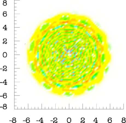
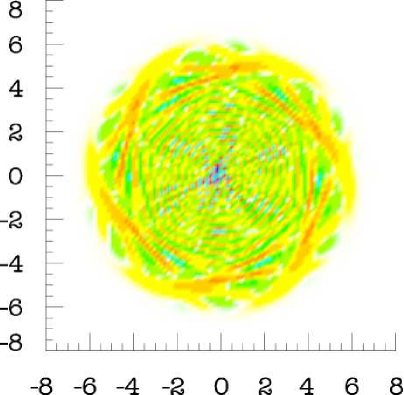
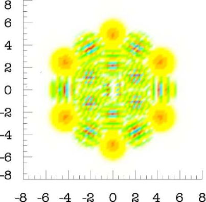
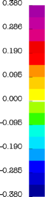
Figure 3: (Color online) For the evolution parameter values close to $\tau=2\pi R$, where $R<1$ is a rational number, in some ares a destructive and in the other a constructive interference starts to dominate – the left ($\tau=0.6$) and the middle figure ($\tau=1$), thus leading to a Wigner function of a coherent superposition state – the right figure ($\tau=\pi/3$). Figures evaluated for $\alpha=5$.

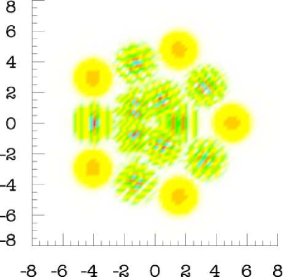
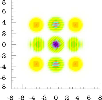
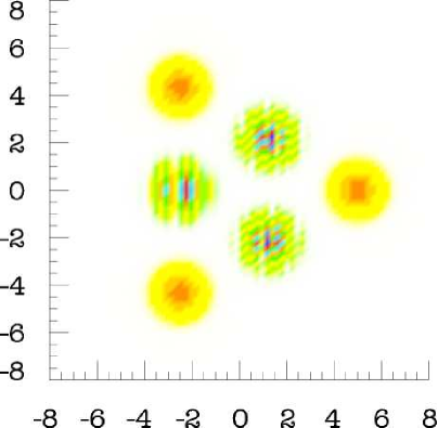
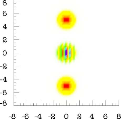
Figure 4: (Color online) The superposition states obtained for $\alpha=5$ and $\tau=2\pi/5$ – the left figure, $\tau=\pi/2$ (the compass state) – the left middle figure, $\tau=2\pi/3$ – the right middle figure and $\tau=\pi$ (the Schrödinger cat state) – the right figure.

Figures 1, 2, 3, 4 present the plots of the Wigner function for different parameters $\tau$ and $\alpha=5$. Due to the fact that the number operator $a^{\dagger}a$ is a constant of motion, the probability distribution during its evolution will remain situated within a circle of radius $|\alpha|$. Beginning from a circular shape, the Wigner function turns into an ellipse and squeezing appears in an appropriate direction. Then the ellipse changes into a banana shape and a “tail” of the interference fringes appears where the distribution takes the negative values. Squeezing increases and the state becomes non-Gaussian. The “banana part” of the distribution gets thinner in the radial direction and becomes more and more smeared in the azimuthal direction.

The rotation and stretching effects which lead to squeezing are revealed by the first term in the first line of the equation (3). It shows the dependence of the angular velocity on the distance $r$ from the origin of coordinates. This corresponds to the fact that the nonlinear refractive index $n(\gamma)$ of Kerr medium is intensity dependent $n(\gamma)=n_{0}+n_{2}|\gamma|^{2}$. The intensity fluctuations modulate the nonlinear refractive index and this in turn modulates the phase of traveling light. Photons with stronger amplitude will acquire phase faster than the photons with smaller amplitude.

The other first line terms of this equation consisting of mixed and third order derivatives are responsible for the interference fringes formulation.

If $\tau$ is taken as a fraction of the period of the evolution, $\tau=2\pi R$ where $R<1$ is a rational number, the initial coherent state becomes a superposition of other coherent states, of the same amplitude but different phases, see fig. 4 OSID . This is is also known as a fractional revival Averbukh1989 .

The evolution governed by the self-Kerr interaction Hamiltonian is periodic. It is easy to see this using a unitary evolution operator $U(\tau)=\exp\{-iHt/\hbar\}$ rather than the Fokker-Planck equation approach. Its action on a coherent state $|\alpha\rangle$ expressed in the Fock state basis

$$|\Psi(\alpha,\tau)\rangle=U(\tau)|\alpha\rangle=e^{-\frac{|\alpha|^{2}}{2}}\sum_{n=0}^{\infty}\,\frac{\alpha^{n}}{\sqrt{n!}}\,e^{i\frac{\tau}{2}n(n-1)}|n\rangle$$ (4)

shows that $|\Psi(\alpha,\tau)\rangle=|\Psi(\alpha,\tau+2\pi)\rangle$. In particular, for $\tau=2k\pi$ where $k$ is an integer, equation (4) reduces again to the coherent state $|\alpha\rangle$. The same periodicity holds for the Wigner function. This condition has been used as an additional check point in our numerical simulations.

For the wave function given by equation (4) one can determine the Wigner function as an analytical function of the evolution parameter $\tau$ using the definition Scully

$$W(\tau,\gamma)\!=\!\frac{2}{\pi^{2}}e^{2|\gamma|^{2}}\!\!\int\!\!d^{2}\beta\langle-\beta|\rho(\alpha,\tau)|\beta\rangle e^{-2(\beta\gamma^{*}-\beta^{*}\gamma)},$$ (5)

where $\rho(\alpha,\tau)$ is the density operator of the state $|\Psi(\alpha,\tau)\rangle$. We apply the above equation and express it in two equivalent ways which have been used to obtain the numerical results for the nondissipative Kerr medium

$$W(\tau,\gamma) = \frac{2}{\pi}\,e^{-2|\gamma|^{2}}e^{-|\alpha|^{2}}\,\sum_{q=0}^{\infty}\frac{\left(2\alpha^{*}\gamma e^{i\frac{\tau}{2}}\right)^{q}}{q!}e^{-i\frac{\tau}{2}q^{2}}$$ (6)

$$\times \sum_{k=0}^{\infty}\frac{\left(2\alpha\gamma^{*}e^{-i\frac{\tau}{2}}\right)^{k}}{k!}e^{i\frac{\tau}{2}k^{2}}e^{-|\alpha|^{2}e^{i\tau(k-q)}},$$

$$W(\tau,\gamma) = \frac{2}{\pi}\,e^{2|\gamma|^{2}}e^{-|\alpha|^{2}}\,\sum_{n,m=0}^{\infty}\frac{1}{(-2)^{n+m}}\frac{\alpha^{n}}{n!}\frac{{\alpha^{*}}^{m}}{m!}$$

$$\times e^{i\frac{\tau}{2}\left[n(n-1)-m(m-1)\right]}\left(\partial_{\gamma}\right)^{n}\left(\partial_{\gamma^{*}}\right)^{m}e^{-4|\gamma|^{2}}.$$

The equations (4) and (LABEL:derivatives) explain how the interference fringes arise from the interference of the Fock number states $|n\rangle$. By virtue of equation (LABEL:derivatives), the Wigner function can be viewed as a sum of the two components: the first one, independent of $\tau$, being a superposition of the Fock states’ Wigner functions $W_{|n\rangle\langle n|}(\gamma)$ and the second, being an evolution dependent component $f(\tau,\gamma)$, responsible for the evolution of the fringes

$$W(\tau,\gamma)=\frac{e^{-|\alpha|^{2}}}{\pi}\sum_{n=0}^{\infty}\frac{|\alpha|^{2n}}{n!}\;W_{|n\rangle\langle n|}(\gamma)+f(\tau,\gamma).$$ (8)

Although the equation (6) and (LABEL:derivatives) are special solutions of the Fokker-Planck equation, we obtained them separately to proceed independent computation.

The effects of squeezing and error contour rotation in the phase space can also be observed by studying the easy-to-compute Q-function evolution $Q(\tau,\gamma)=1/\pi\langle\gamma|\rho(\alpha,\tau)|\gamma\rangle$

$$Q(\tau,\gamma)=\frac{1}{\pi}e^{-|\alpha|^{2}-|\gamma|^{2}}\left|\sum_{n}\frac{(\alpha\gamma^{*})^{n}}{n!}\,e^{i\frac{\tau}{2}n(n-1)}\right|^{2}.$$ (9)

The contour plot of the Q-function is plotted in Tanas . Solutions of the Fokker-Planck equation for the Q-function in a dissipative and noisy Kerr medium have been widely studied Tanas ; Milburn1986 ; Milburn1989 ; Perinova1990 . Negativities achieved in the Wigner function correspond to zeros of the Q-function Korsch1997 .

All the figures 1–4 have been obtained computing the equations (3), (6) and (LABEL:derivatives) independently.

IV Dissipation effects

In the presence of damping the Wigner function will not remain situated within at the circle of the radius $|\alpha|$ any more. The second line in the Fokker-Planck equation, proportional to the first radial derivative, makes the Wigner function moving towards the origin of the coordinates. This effect corresponds to decreasing number of quanta in the state during the evolution. At the origin the state becomes vacuum.

The third line describes the effects of dispersion.

It is interesting to note an interplay between the nonlinear evolution and damping terms in the Fokker-Planck equation. If damping is negligible, the numerical simulations obtained for small $|\alpha|\simeq 1$ and large $|\alpha|\gg 1$ initial amplitudes are very similar. At the beginning of evolution the squeezing effect dominates and then the interference appears. It is not the case if the losses are included in the simulations. If the amplitude is too small the decoherence washes out all the quantum effects and the Gaussian Wigner function located at the coordinates’ origin, genuine to vacuum state, is obtained very quickly.

We proceed the numerical computation for experimentally reasonable values genuine to a nanomechanical resonator. The nonlinear constant $\kappa\simeq 2\cdot 10^{-4}\mathrm{s^{-1}}$ and the damping constant $\Gamma\simeq 10^{3}\,\mathrm{s^{-1}}$ ($\xi=10^{5}$). The thermal noise coefficient in the room temperature is equal to $N\simeq 1.9\cdot 10^{-14}$.

The nonlinear evolution term $r^{2}$ for $\tau\simeq 0$ becomes meaningful if $r\simeq|\alpha|$. If $|\alpha|\simeq 1$ the damping term $\frac{\xi r}{2}\simeq 0.5\cdot 10^{5}$ dominates over the nonlinear $r^{2}\simeq 1$ and interference terms. The coherent state will be almost immediately radially displaced towards the origin of coordinates. For $|\alpha|\simeq 10^{5}$ all the effects are in balance: $r^{2}\simeq 10^{10}$ and $\frac{\xi r}{2}\simeq 0.5\cdot 10^{10}$.

Computing the Fokker-Planck equation for such large values of coefficients ($\alpha\simeq 10^{5}$, $\xi\simeq 10^{5}$, $N=1.9\cdot 10^{-14}$) would require a very dense and large grid, thus a lot of computer memory. Therefore, to visualize an influence of these two effects on the Wigner function, we rescaled the parameters.

As we pointed out above, in order to see the nonlinear effects during the Wigner function evolution in presence of dissipation, the input of nonlinear term has to be of the same order as the dissipation term is. Therefore, we keep the ratio between them constant and equal to the ratio evaluated for the non-rescaled case: $\xi\simeq\alpha$ and $N=1.9\cdot 10^{-19}\xi$. For $\alpha=2$ they are equal to $\xi\simeq 2$ and $N=3.8\cdot 10^{-19}$. Although such a small value of the thermal coefficient implies a negligible effect on the evolution, we included it in the simulation. Such simulations are accessible using a standard PC computer with 4 GB of memory.

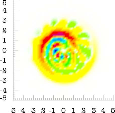
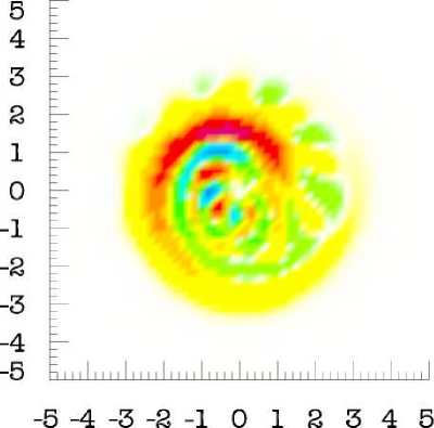
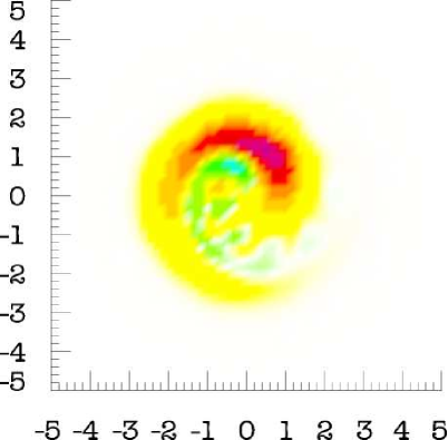
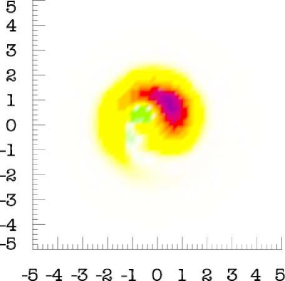
Figure 5: (Color online) The effect of the decoherence on the Wigner function evaluated for $\alpha=2$, $\tau=0.2\pi$, the thermal noise $N=3.8\cdot 10^{-19}$ and the different values of the damping constant: $\xi=0$ – the left figure, $\xi=0.1$ – the left middle figure, $\xi=1$ – the right middle figure, $\xi=2$ – the right figure. Note that the thermal noise gives no input if $\xi=0$.

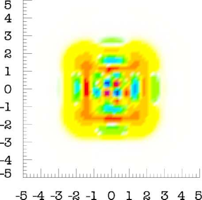
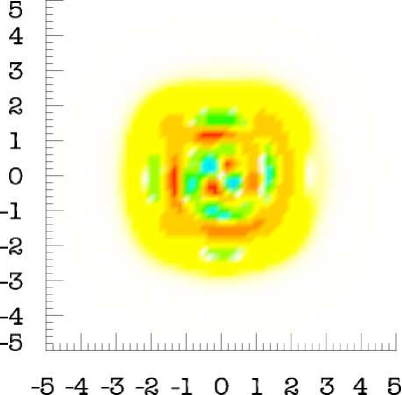
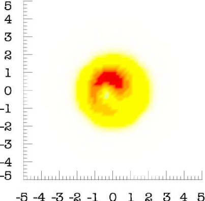
Figure 6: (Color online) The coherent superposition states are extremely fragile to the decoherence process. The Wigner function of four coherent state superposition ($\tau=\pi/2$) of the amplitude $\alpha=2$ evaluated including the thermal noise $N=3.8\cdot 10^{-19}$ and the damping constant equal to $\xi=0$ – the left figure, $\xi=0.1$ – the left middle figure, $\xi=1$ – the right middle figure, $\xi=2$ – the right figure.

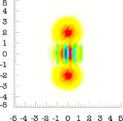
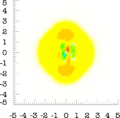
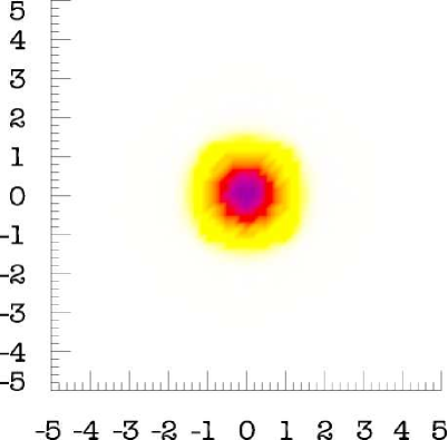
Figure 7: (Color online) The decoherence looks similarly for the two coherent state superposition Wigner function ($\tau=\pi$), also of amplitude $\alpha=2$, the same thermal noise $N=3.8\cdot 10^{-19}$ and the damping constants: $\xi=0$ – the left figure, $\xi=0.1$ – the left middle figure, $\xi=1$ – the right middle figure, $\xi=2$ – the right figure.

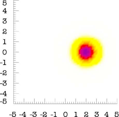
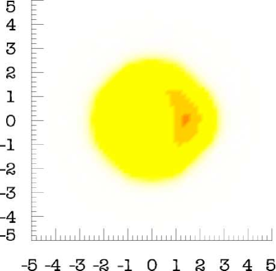
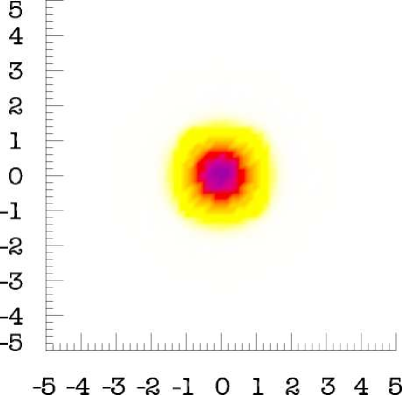
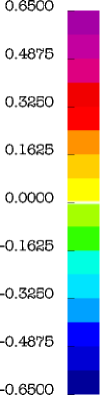
Figure 8: (Color online) The Wigner function evolution is a noisy $\chi^{(3)}$ medium is not periodic any more. The distribution evaluated for $\alpha=2$, $\tau=2\pi$, the thermal noise $N=3.8\cdot 10^{-19}$ and the damping constant equal to $\xi=0$ – the left figure, $\xi=0.1$ – the middle figure, $\xi=1$ – the right figure. The state pursues vacuum.

Figures 5, 6, 7, 8 present the numerical simulations of the Fokker-Planck equation obtained for $\alpha=2$, $N=3.8\cdot 10^{-19}$ and the following values of the damping constant: $\xi=0$, $\xi=0.1$, $\xi=1$, $\xi=2$.

Due to the fact that damping washes out the interference effects, any nonzero damping constant prevents both: coherent superposition state formulation and periodicity of the evolution. As it is well known Zurek these states are extremely fragile to the decoherence. The areas where the Wigner function takes the negative values disappear, see fig. 5. For an ideal $\chi^{(3)}$ medium the negativities show up for $0.08+2k\pi<\tau<6.20+2k\pi$ where $k$ is an integer. If $\xi=0.1$ the negativities are present for $0.08<\tau<5.80$. However, they do not appear in the second round ($0.08+2\pi<\tau<5.80+2\pi$). If $\xi=1$ the negative values are present only for $0.08<\tau<1.52$ and for $0.08<\tau<0.89$ if $\xi=2$.

The Wigner function obtained for the coherent superposition states evolution times $\tau=\frac{\pi}{2}$, $\tau=\pi$ and $\tau=2\pi$ is depicted on figures 6, 7, 8. For $\xi=0.1$ the structure of superposition coherent states is still well preserved. However, some additional circular trails are present. These are specially visible for $\tau=\pi$ and $\tau=2\pi$. For $\xi=2$ and $\tau=\frac{\pi}{2}$ the state is already a vacuum. The vacuum state is achieved for $\tau=\pi$ ($\tau=10\pi$) if $\xi=1$ ($\xi=0.1$).

V Sub-Planck structure in phase-space

In the framework of quantum mechanics, it has been recognized that small structures on the sub-Planck scale do show up in quantum linear superpositions ZurekN ; ZurekPRA . Such sub-Planck structures can be shown, if the Wigner function is plotted in a phase-space region below the Heisenberg relation. That means in the phase space volume less than $1$, since $\Delta X_{1}\Delta X_{2}\geq 1$ for the amplitude $X_{1}$ and phase $X_{2}$ quadratures. The quadratures are given by the annihilation $a=\frac{1}{2}(X_{1}+iX_{2})$ and creation $a^{\dagger}=\frac{1}{2}(X_{1}-iX_{2})$ operators and their mean values correspond to phase-space coordinates in the following way $\langle X_{1}\rangle=\mathrm{Re}\,\gamma$, $\langle X_{2}\rangle=\mathrm{Im}\,\gamma$.

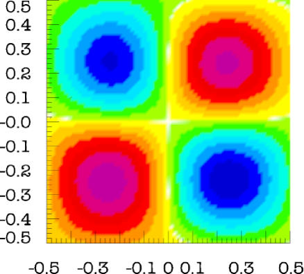
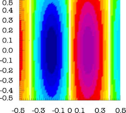
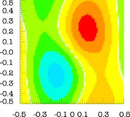
Figure 9: (Color online) A sub-Planck structure of the Wigner function for $\tau=\pi/2$ and $\xi=0$ – the left figure, $\tau=\pi/2$ and $\xi=0.1$ – the left middle figure, $\tau=\pi$ and $\xi=0$ – the right middle figure, $\tau=\pi$ and $\xi=0.1$ – the right figure.

Figure 9 compares behavior of the sub-Planck structure of the Wigner function obtained for the compass state ($\tau=\pi/2$) and the Schrödinger cat state ($\tau=\pi$) for $\alpha=2$ in the ideal $\chi^{(3)}$ medium and in presence of damping ($\xi=0.1$). The regions of the opposite sign, in the form of “dots,” are clearly visible. They become flattened and smeared by the damping effects.

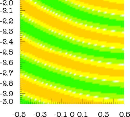
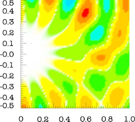
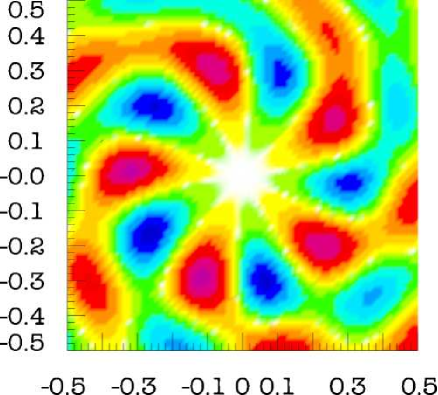
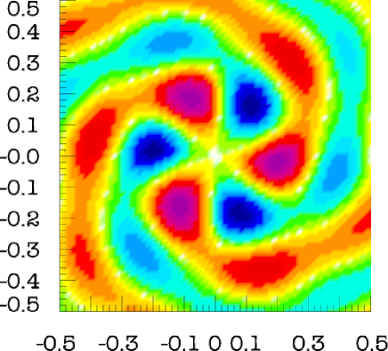
Figure 10: (Color online) A sub-Planck structure of the Wigner function evaluated for $\tau=0.16$, $\tau=0.3$, $\tau=0.6$, $\tau=1$.

The sub-Planck structure is also present for the rational values of evolution parameter, for which the state (4) does not correspond to any coherent superposition state. It is depicted on figure 10 for $\tau=0.16$, $\tau=0.3$, $\tau=0.6$, $\tau=1$ and $\alpha=5$. This structure is of different form. The areas of positive and negative values form “ribbons.”

VI Comparison of the Numerical Methods

Figures 1–4, presenting the Wigner function evolution in an ideal $\chi^{(3)}$ medium, have been obtained by three independent numerical simulations: computing of the equations (3), (6) and (LABEL:derivatives). The numerical results of the evolution in a noisy medium have been achieved using only the Fokker-Planck equation (3).

All programs used to simulate the Wigner function were written in standard C++ language, due to its high speed and good portability. The structure of the programs used for computation of the equations (6) and (LABEL:derivatives) was based strictly on these equations: they both consist of two loops which iterate on $q$ and $k$ (or $m$ and $n$, respectively) and sum up the evaluated coefficients for a given $\tau$ and $\gamma$. Common terms were moved out from the loops (especially the inner one) to optimize the evaluation of the sums. The main function was enclosed in input/output logic which calls it for different values of $\gamma$ and writes the results to a file.

The equations (6) and (LABEL:derivatives) involve summation of the infinite series. However, only a finite number of their terms can be computed. Therefore, assuming a given precision of the simulation, we cut the series off.

The series in equation (6) is much slower convergent than the series in (LABEL:derivatives) because it contains fast oscillating exponential term $e^{-|\alpha|^{2}e^{i\tau(k-q)}}$. Depending on the phase factor in the exponent, this term can take either large or small values, which makes impossible to compute equation (6) using the standard double precision floating point number representation. Therefore, for $|\alpha|\leq 5$ both infinite sums, internal and external, are cut off by including at least $500$ terms in each of them. Also very high precision (at least 25 significant digits) needs to be applied for the computation. Such a high precision was obtained using the free Class Library for Numbers (CLN) and its long float type.

On contrary, it is enough to use standard double precision numbers to compute equation (LABEL:derivatives). However, we also applied the CLN here due to the fact that it can deal with the complex numbers while C++ itself cannot. The same precision was used while computing equation (LABEL:derivatives) however, it was enough to take $100$ terms in both sums into account to obtain the same results as these which were achieved by computing (6). This made simulations of equation (LABEL:derivatives) much faster. Additionally, the product of the exponens derivatives was replaced with the following formula bronstein

$$(\partial_{\gamma})^{n}(\partial_{\gamma^{*}})^{m}e^{-4|\gamma|^{2}} = \sum_{k=0}^{n}{n\choose k}(\partial_{\gamma})^{k}(-4\gamma)^{m}(\partial_{\gamma})^{n-k}e^{-4|\gamma|^{2}}$$ (10)

$$= e^{-4|\gamma|^{2}}\sum_{k=0}^{\mathrm{min}(n,m)}{n\choose k}\frac{m!}{(m-k)!}$$

$$\times (-4\gamma)^{m-k}(-4\gamma^{*})^{n-k}.$$

Both methods, equations (6) and (LABEL:derivatives), allow for computation of the Wigner function for an arbitrary evolution parameter $\tau$ and point $\gamma$ in the phase space. Evaluation of the function for a chosen $\tau$ does not require simulation of the whole evolution. To visualize the Wigner function we calculated it for each point of a $100\times 100$ square mesh of the size proportional to the value of $\alpha$ ($-5\ldots 5$ for $\alpha=2$, $-8\ldots 8$ for $\alpha=5$, $-\frac{1}{2}\ldots\frac{1}{2}$ for sub-Planck structures), to show all interesting aspects of the simulated function.

On the contrary, numerical simulation of the Fokker-Planck equation (3) involves solving a partial differential equation (PDE), which in turn requires setting a grid (discretized phase space) and solving a set of linear equations (one equation for each point of the grid) at each time step.

To solve the PDE, the equation (3) was rewritten to difference quotient form, where all the partial derivatives were replaced with appropriate difference quotients of fourth order to keep the order of the quotients even and higher than the order of the equation at the same time. Even difference quotients are more convenient, since they are symmetric with respect to the point where the derivative is taken. The quotients were determined using the Mathematica program and its FiniteDifferencePolynomial function. We used polar mesh coordinates with constant radial distance $\Delta r$ and constant angle $\Delta\varphi$ between points. Below we present the first, second and third derivatives discretized up to the forth order:

$$\partial_{x} \rightarrow \frac{f_{k-2}-8f_{k-1}+8f_{k+1}-f_{k+2}}{12h}$$ (11)

$$\partial^{2}_{x} \rightarrow \frac{-f_{k-2}+16f_{k-1}-30f_{k}+16f_{k+1}-f_{k+2}}{12h^{2}}$$ (12)

$$\partial^{3}_{x} \rightarrow \frac{-f_{k-2}+2f_{k-1}-2f_{k+1}+f_{k+2}}{2h^{3}}$$ (13)

where $x=r,\varphi$, $h=\Delta r,\Delta\varphi$ and $k=i,j$ for $r$ and $\varphi$ respectively, $f_{k}$ is the Wigner function value. The mixed derivatives where built up combining the basic above formulas.

Since the standard explicite computation methods turned out to be unstable due to large number of time steps, we applied implicite method. At the same time, it also allowed for larger time steps. The main idea of implicite method is to determine the time derivative between steps $\tau$ and $\tau+\Delta\tau$ using the spatial derivatives obtained from the next time step $W(\tau+\Delta\tau,\gamma,\gamma^{*})$, not from the previous one $W(\tau,\gamma,\gamma^{*})$. This method requires solving a set of linear equations, with Wigner function values in the next time step $W(\tau+\Delta\tau,\gamma,\gamma^{*})$ for each point $\gamma$ of the mesh as unknowns. The stability of this method relies on well-chosen ratio of the time step and the grid density. For $\alpha=2$ we used time step $\Delta\tau=\frac{\pi}{3600}$ and the grid consisting of $300\;(\mathrm{radial\;direction})\times 540\;(\mathrm{azimuthal\;direction)}$ points. Thus, there were $162\cdot 10^{3}$ points and equations in the set.

In order to solve such a large set of equations, we put it in a matrix form. To achieve it we assigned an index $i$ for each point of the polar mesh using the formula $i=N_{f}\,r/\Delta r+\varphi/\Delta\varphi$, where $N_{f}$ is a density of the grid in azimuthal direction, $r$ and $\varphi$ are polar coordinates of a point of the mesh and $\Delta r$ and $\Delta\varphi$ are radial and angular distances between mesh points. This index was then used as a coordinate to the row and column of the matrix where the coefficients of the equations were placed and to rewrite the Wigner function values of the previous time step from grid to vector form and the result from vector back to mesh form.

The index $i$ (described above) was chosen in such a way that the matrix of equation coefficients is a sparse band matrix. The sample of such matrix computed for small mesh size is depicted on fig. 11. Black points represent nonzero items (single numbers). It consists of five diagonal five-element bands and additional two including either two or one element. In practice, the matrix is much larger and has $162\cdot 10^{3}\times 162\cdot 10^{3}$ elements, but the characteristic band diagonal structure with five-element bands is preserved.

The set of equations is solved using Band Diagonal Systems method nume : the matrix is inverted applying LU decomposition (Crout method) and then solved with Gaussian elimination while keeping the matrices in special compressed form to save computer memory. We used the bandec and banmul routines from nume , translated to C++ and optimized. We also used standard double precision floating point numbers; there was no need for CLN library. The main computing routine was accompanied by input/output logic used to read simulation parameters and write out the results.

The flow of the program consisted of an introductory step – performing a LU decomposition and calculating Wigner function for $\tau=0$ (initial values for each point of the grid) – and a sequence of steps calculating evolution of the Wigner function for each $\tau=\tau_{0}+n\Delta\tau$. The solution gives the values of the function for all $\gamma$ at each evolution step.

During the simulation some sanity checks were taken to make sure that the calculations are done properly, e.g. the integral of the Wigner function over the phase space is equal to 1 in each time step. The value of the integral unequal to 1 was a sign of either too small mesh density or too big time step or too small precision of the calculations. We also compared the results of simulation of equations (3), (6) and (LABEL:derivatives) for the same input parameters.

The numerical results are presented using OpenDX program.

VII Conclusion

In this paper we presented the Fokker-Planck equation which allowed for numerical computation of the full Wigner function evolution governed by the self-Kerr interaction Hamiltonian. This equation can be used for a state analysis for any input state, mixed or pure. We took a coherent state as an input state for the simulation. For a decoherence-free evolution the results have been obtained by three different numerical algorithms. We discussed the influence of the decoherence process on the nonclassicality of the state under evolution. For an exemplary calculation we took into consideration the experimentally reasonable values of the nonlinearity and damping constant for a nanomechanical resonator. We also presented the sub-Planck structure of the Wigner function which arises during the evolution. This equation can be applied to any system described by the self-Kerr interaction.

This work was partially supported by a MEN Grant No. 1 PO3B 137 30 (K.W.) and N202 021 32/0700 (M.S.).

Figure 11: The sparse band matrix necessary to invert to solve the set of linear equations giving the Wigner function values for all points of the discretized phase space.

References

- (1) L. Praxmeyer, P. Wasylczyk, C. Radzewicz, and K. Wódkiewicz, Phys. Rev. Lett. 98, 063901 (2007).
- (2) S.-B. Li, X.-B. Zou, and G.-C. Guo, Phys. Rev. A75, 045801 (2007).
- (3) A. Biswas and G. S. Agarwal, Phys. Rev. A75, 032104 (2007).
- (4) A. Ourjoumtsev, A. Dantan, R. Tualle-Brouri, and Ph. Grangier, Phys. Rev. Lett. 98, 030502 (2007).
- (5) A. Ourjoumtsev, R. Tualle-Brouri, and Ph. Grangier, Phys. Rev. Lett. 96, 213601 (2006).
- (6) J. S. Neergaard-Nielsen, B. Melholt Nielsen, C. Hettich, K. Molmer, and E. S. Polzik, Phys. Rev. Lett. 97, 083604 (2006).
- (7) H. Jeong, A. P. Lund, and T. C. Ralph, Phys. Rev. A72, 013801 (2005).
- (8) I. Katz, A. Retzker, R. Straub, and R. Lifshitz, Phys. Rev. Lett. 99, 040404 (2007).
- (9) P. Weetman and M. S. Wartak, Phys. Rev. B76, 035332 (2007).
- (10) E. Wigner, Phys. Rev. 40, 749 (1932).
- (11) N. Imoto, H. A. Haus, and Y. Tamamoto Phys. Rev. A32, (1985).
- (12) Q. A. Turchette, C. J. Hood, W. Lange, H. Mabuchi, and H. J. Kimble Phys. Rev. Lett. 75, 4710 (1995).
- (13) A. K. Mohapatra, M. G. Bason, B. Butscher, K. J. Weatherill, and C. S. Adams, quant-ph/0804.3273v1.
- (14) A. Imamoglu, H. Schmidt, G. Woods, and M. Deutsch Phys. Rev. Lett. 79 1467 (1997). M. J. Werner and A. Imamoglu Phys. Rev. A61 011801 (1999).
- (15) L. V. Hau, S. E. Harris, Z. Dutton, and C. H. Behroozi, Nature 397 594 (1999).
- (16) H. Kang and Y. Zhu, Phys. Rev. Lett. 91 093601 (2003).
- (17) P. Bermel, A. Rodriguez, J. D. Joannopoulos, and M. Soljacic, Phys. Rev. Lett. 99, 053601 (2007).
- (18) F. G. S. L. Brandao, M. J. Hartmann, and M. B. Plenio, New J. Phys. 10 043010 (2008).
- (19) M. J. Woolley, G. J. Milburn, and Carlton M. Caves, quant-ph:0804.4540v1; E. Babourina-Brooks, A. Doherty, G. J. Milburn, quant-ph:0804.3618v1.
- (20) I. Kozinsky, H. W. Ch. Postma, O. Kogan, A. Husain, and M. L. Roukes, Phys. Rev. Lett. 99, 207201 (2007).
- (21) R. Tanaś, Nonclassical states of light propagating in Kerr media, in Theory of Non-Classical States of Light, V. Dodonov and V. I. Man’ko eds., Taylor and Francis, London 2003.
- (22) D. F. Walls, G. J. Milburn, Quantum Optics, Springer-Verlag Berlin and Heidelberg GmbH and Co. KG (1995).
- (23) G. J. Milburn and C. A. Holmes, Phys. Rev. Lett. 56, 2237 (1986).
- (24) D. J. Daniel and G. J. Milburn, Phys. Rev. A39, 4628 (1989).
- (25) V. Perinova and A. Luks, Phys. Rev. A41, 414 (1990).
- (26) C. W. Gardiner, Quantum Noise, (Springer-Verlag, Berlin, 1991).
- (27) M. Stobińska, G. J. Milburn, and K. Wódkiewicz, OSID 14, 81 (2007).
- (28) I. Sh. Averbukh and N. F. Perelman, Phys. Lett. 139, 449 (1989).
- (29) M. O. Scully and M. S. Zubairy, Quantum Optics, Cambridge University Press (1997).
- (30) H. J. Korsch, C. Muller, and H. Wiescher, J. Phys. A 30, L677 (1997).
- (31) I. L. Chuang, R. Laflamme, P. W. Shor, W. H. Zurek, Science 270, 1633 (1995).
- (32) F. Toscano, D. A. R. Dalvit, L. Davidovich, and W. H. Zurek, Nature 412, 712 (2001).
- (33) W. H. Zurek, Phys. Rev. A63, 023803 (2006).
- (34) I. N. Bronstein, K. A. Semendiajew, Taschenbuch der Mathematik, (B. G. Teubner Verlagsgesellshaft, Leipzig 1959).
- (35) W. H. Pres, B. P. Flannery, S. A. Teukolsky, and W. T. Vetterling, Numerical Recipes (Cambridge University Press, Cambridge, 1988).