Universal role of correlation entropy in critical phenomena

Abstract

In statistical physics, if we successively divide an equilibrium system into two parts, we will face a situation that, within a certain length $\xi$, the physics of a subsystem is no longer the same as the original system. Then the extensive properties of the thermal entropy $S($AB$)=S($A$)+S($B$)$ is violated. This observation motivates us to introduce the concept of correlation entropy between two points, as measured by mutual information in the information theory, to study the critical phenomena. A rigorous relation is established to display some drastic features of the non-vanishing correlation entropy of the subsystem formed by any two distant particles with long-range correlation. This relation actually indicates the universal role of the correlation entropy in understanding critical phenomena. We also verify these analytical studies in terms of two well-studied models for both the thermal and quantum phase transitions: two-dimensional Ising model and one-dimensional transverse field Ising model. Therefore, the correlation entropy provides us with a new physical intuition in critical phenomena from the point of view of the information theory.

I Introduction

Entropy is one of the most important concept in both statistical physics Khuangb and information theory Shannon48 ; TMCover91b ; Nielsenb . It measures how much uncertainty there is in a state of physical system. In statistical physics, the entropy defined by $S=\log_{2}\Omega$ depends on the number of states $\Omega$ in an equilibrium system; while in the information theory, the entropy $S=-{\rm tr}(\rho\log_{2}\rho)$ is associated with the probability distribution in the eigenstate space of the density matrix $\rho$. Therefore, it is interesting to look into some fundamental issues from different point of view due to the common ground of two fields.

In statistical physics, if we divide an equilibrium system into a large number of macroscopic parts, the total number of state in phase space is a product form from the number $\omega_{i}$ of state in each part, i.e. $\Omega=\prod_{i}\omega_{i}$. This precondition leads to that the entropy is an extensive quantity in statistical physics, i.e. $S=\sum_{i}S_{i}$, which is one of basis of the second law of the thermodynamics. However, a realistic system includes all kinds of interaction, and the dynamics at one site is no longer independent of other sites nearby. The facts implies that if we successively divide a system into two parts, we will face a situation that, within a certain length $\xi$, the physics of a subsystem is not the same as the original system. This length actually defines a characteristic scale for the statistical physics, and physicists usually call it correlation length in the studying of different kinds of correlation function. From the point view of the information theory, for two subsystems A and B within the length scale $\xi$, they are no longer independent with each other, and their entropy does not satisfy the extensive property, i.e. $S($AB$)\neq S($A$)+S($B$)$.

On the other hand, correlation function plays a fundamental role in physics. Almost all physical quantities, not only in condensed matter physics, but also in quantum field theory, are related to the correlation function either directly or indirectly. Thus it devotes to understand many phenomena in both classical and quantum mechanics. Physically, the correlation function denotes the amplitude of the dependence of physical variables between two points in space time. From the information theory, it also partially measures how much uncertainty of a physical quantity at one location if the quantity at another one is given. However, this uncertainty still depends on the quantity itself. For example, in quantum system, the diagonal correlation function usually differs from the off-diagonal correlation function. Therefore, in order to learn the dependence between two separated systems, it is important to ask such a question: to what extent that the equality $S($AB$)=S($A$)+S($B$)$ is violated. This question introduces a concept in the information theory, i.e. mutual information, which is defined as

$$S({\rm A:B})=S({\rm A})+S({\rm B})-S({\rm AB})$$ (1)

where $S(i)=-{\rm tr}(\rho_{i}\log_{2}\rho_{i}),i={\rm A,B,AB}$ is the entropy of the corresponding reduced density matrix. If $\rho$ is classical, it is the Shannon entropy Shannon48 , otherwise it is the von Neumann entropy AWehrl78 of the quantum information theory. Actually, all correlation functions $\langle O_{\rm A}O_{\rm B}\rangle$ between A and B can be calculated from the reduced density matrix $\rho_{\rm AB}$, i.e. $\langle O_{\rm A}O_{\rm B}\rangle={\rm tr}\langle O_{\rm A}O_{\rm B}\rho_{\rm AB}\rangle$. The mutual information, which measures the common shared information, defines a more general operator-independent correlation between two subsystems. Taking into account the role of entropy in the statistical physics, we would like to call it correlation entropy hereafter.

To have a concrete interpretation, it is useful return to intuitive understanding of the entropy itself. In the information theory, the entropy is used to quantify the physical resource (in unit of classical bit due to $\log_{2}$ in its expression) needed to store information. For example, in the exact diagonalization approach, if we want to diagonalize a Hamiltonian of 10-site spin-1 chain and no symmetry can be used to reduce the dimension of the Hilbert space, we need at least $S=\log_{2}3^{10}=10\log_{2}3$ bits to store a basis. Therefore, the correlation entropy actually measures the additional physical resource required if we store two subsystems respectively rather than store them together. As a simple example, let us consider a two-qubit system in a singlet state $(|\uparrow\downarrow\rangle-|\downarrow\uparrow\rangle)/\sqrt{2}$, we have $S($A$)=1,S($B$)=1,S($AB$)=0$, which leads to $S($A: B$)=2$. Obviously, there is no information in a given singlet state. However, each spin in this state is completely uncertain. So we need two bits to store them respectively. On the other hand, the correlation entropy is simply the twice of the entanglement, as measured by partial entropy, between two systems because of $S($A$)=S($B$)$ for pure state. The reason that we interpret the correlation entropy in this way is that besides the quantum correlation the state also has classical correlation. From this point of view, the correlation entropy is just a measure of total correlation, including quantum and classical correlation, between two subsystems. They go halves with each other in correlation entropy for pure state. For a mixed state, the correlation entropy also measures the amount of the uncertainty of one system before we learn one from another. From the above interpretation for pure state, it is then not surprising that the correlation entropy fails to measure the entanglement VVedral1997 .

In the statistical physics, the critical phenomena is the central topic. To have a complete understanding on the critical behavior, various methods, such as renormalization group Rshankar94 , Monte-Carlo simulation DPLandaub , and mean-field approach etc., have been developed and applied to many kinds of systems. In recent years, the study on the role of entanglement in the quantum critical behavior Sachdev have established a bridge between quantum information theory and condensed matter physics, and shed new light on the quantum phase transitions due to its interesting behavior around the critical point AOsterloh2002 ; TJOsbornee ; SJGuXXZ ; SJGUPRL ; Aanfossi05 ; HTQuan06 . However, the entanglement is fragile under the thermal fluctuation and can be suppressed to zero at finite temperatures. Then it is difficult to witness a generalized thermal phase transition in terms of quantum entanglement.

In this paper, we are going to study the role of correlation entropy in both thermal and quantum phase transitions. Like the fundamental role of two point correlation function in the statistical physics, we are interested in the universal role of two-point correlation entropy in the present work. The paper is organized as follows. In Sec. II, for the pedagogical purpose, we study a toy model and show that the thermal entropy is not an extensive parameter in such a simple system. In Sec. III, we discuss the relation between the reduced density matrix, long-range correlation, and the correlation entropy. In Sec. IV, we study the properties of the correlation entropy in thermal phase transition, as illustrated by classical two-dimensional Ising model. In Sec. V, we address the properties of the correlation entropy in a simple quantum phase transition of one-dimensional transverse field Ising model. In Sec. VI, some discussions and prospects are presented. Finally, a brief summary is given in Sec. VII

II Toy model: Heisenberg dimer

For the pedagogical purpose and making our motivation more clear, we first have a look on a very simple model: a Heisenberg dimer. Its Hamiltonian reads

$$H=\sigma_{1}\cdot\sigma_{2}$$ (2)

where $\sigma_{i}(\sigma^{x},\sigma^{y},\sigma^{z})$ are Pauli matrices at site $i$,

$$\sigma^{x}=\left(\begin{array}[]{cc}0&1\\ 1&0\\ \end{array}\right),\;\sigma^{y}=\left(\begin{array}[]{cc}0&-i\\ i&0\\ \end{array}\right),\;\sigma^{z}=\left(\begin{array}[]{cc}1&0\\ 0&-1\\ \end{array}\right)$$ (9)

and the coupling between two sites is set to unit for simplicity. The Hamiltonian can be diagonalized easily. Its ground state is a spin singlet state

$$\Psi_{0}=\frac{1}{\sqrt{2}}\left[|\uparrow\downarrow\rangle-|\downarrow\uparrow\rangle\right],$$ (10)

with eigenvalue $E_{0}=-3$, while three degenerate excited states are

$$\Psi_{1}=\frac{1}{\sqrt{2}}\left[|\uparrow\downarrow\rangle+|\downarrow\uparrow\rangle\right],$$

$$\Psi_{2}=|\uparrow\uparrow\rangle,\;\;\;\Psi_{3}=|\downarrow\downarrow\rangle.$$ (11)

with higher eigenvalue $E_{1,2,3}=1$. Therefore, according to the statistical physics, the thermal entropy of the system vanishes at zero temperature. When the system is contacted with a thermal bath with temperature $T$, the thermal state of the system is described by a density matrix:

$$\rho=\zeta\left(\begin{array}[]{cccc}e^{-2/T}&0&0&0\\ 0&\cosh(2/T)&-\sinh(2/T)&0\\ 0&\sinh(2/T)&\cosh(2/T)&0\\ 0&0&0&e^{-2/T}\\ \end{array}\right)$$ (16)

where

$$\zeta=\frac{1}{3e^{-2/T}+e^{2/T}}.$$ (17)

Because of SU(2) symmetry of the Heisenberg dimer, the single-site entropy $S(i)$ of the system is always unity, and the entropy of the whole system is

$$S(12)=2-\frac{\log_{2}(3e^{-2/T}+1)}{3e^{-2/T}+1}-\frac{3\log_{2}(3+e^{4/T})}{3+e^{4/T}}.$$ (18)

Then we can see that $S(12)\neq S(1)+S(2)$ both at zero temperature and finite temperatures. In high temperature limit, the asymptotic behavior of the correlation entropy is $S(1:2)\propto 1/T$. So only when $T\rightarrow\infty$, $S(1:2)\rightarrow 0$, the extensive property of the entropy holds. The physics behind this fact is quite clear. It is the interaction between two sites that establishes a kind of correlation and then breaks the extensive property of the entropy.

For a large system, however, this correlation usually decays with the increasing of distance between two parts, and the entropy becomes an extensive quantity beyond a definite scale. Only around the critical point where the phase transition happens, the system behaves like a whole and can not be divided into two part, and then the correlation entropy has long range behaviors.

III reduced density matrix, long-range order, and correlation entropy

In many-body physics, the reduced density matrix of a one-body and two-body subsystem can be, in general, written as

$$\langle\alpha^{\prime}|\rho_{i}|\alpha\rangle={\rm tr}(a_{i\alpha^{\prime}}\rho a^{\dagger}_{i\alpha}),$$

$$\langle\alpha^{\prime}\beta^{\prime}|\rho_{ij}|\alpha\beta\rangle={\rm tr}(a_{i\alpha^{\prime}}a_{j\beta^{\prime}}\rho a^{\dagger}_{j\beta}a^{\dagger}_{i\alpha}),$$ (19)

respectively. Here $a_{i\alpha},a_{j\beta}$ are annihilation operators for states $|\alpha\rangle,|\beta\rangle$ localized at site $i,j$ respectively, and satisfy commutation (anti-commutation) relation for bosonic (fermionic) states. The reduced density matrix is usually normalized as

$${\rm tr}(\rho_{i})=1,\;\;{\rm tr}(\rho_{ij})=1,$$ (20)

so that one has a probability explanation for their diagonal elements in the corresponding eigenstate space.

In spin system, the reduced density matrix of a single spin at position $i$ takes the form

$$\rho_{i}=\frac{1}{2}\big{(}1+\langle\sigma_{i}^{x}\rangle\sigma_{i}^{x}+\langle\sigma_{i}^{y}\rangle\sigma_{i}^{y}+\langle\sigma_{i}^{z}\rangle\sigma_{i}^{z}\big{)}.$$ (21)

For two arbitrary spins at position $i$ and $j$, the two-site reduced density matrix generally takes the form,

$$\rho_{ij} = \frac{1}{4}+\frac{1}{4}\sum_{\alpha}\left(\langle\sigma_{i}^{\alpha}\rangle\sigma_{i}^{\alpha}+\langle\sigma_{j}^{\alpha}\rangle\sigma_{j}^{\alpha}\right)$$ (22)

$$+\frac{1}{4}\sum_{\alpha\beta}\langle\sigma_{i}^{\alpha}\sigma_{j}^{\beta}\rangle\sigma_{i}^{\alpha}\sigma_{j}^{\beta}.$$

Obviously, under some symmetry, the above reduced density matrix can be simplified. For example, if the state of $N$ spins is also an eigenstate of $z$ component of total spins $S^{z}=\sum S_{i}^{z}=0$ and possesses the exchange symmetry, then Eq. (22) can be simplified as

$$\rho_{ij}=\left(\begin{array}[]{cccc}u^{+}&0&0&0\\ 0&w_{1}&z&0\\ 0&z^{*}&w_{2}&0\\ 0&0&0&u^{-}\end{array}\right)$$ (27)

in the basis of $\sigma^{z}_{i}\sigma^{z}_{j}$: $\{|\uparrow\uparrow\rangle$, $|\uparrow\downarrow\rangle$, $|\downarrow\uparrow\rangle$, $|\downarrow\downarrow\rangle\}$. Here the matrix elements can be calculated from the correlation function,

$$u^{+}=u^{-}=\frac{1}{4}(1+\langle\sigma^{z}_{i}\sigma^{z}_{j}\rangle),$$

$$w_{1}=w_{2}=\frac{1}{4}(1-\langle\sigma^{z}_{i}\sigma^{z}_{j}\rangle),$$

$$z=\frac{1}{4}(\langle\sigma^{x}_{i}\sigma^{x}_{j}\rangle+\langle\sigma^{y}_{i}\sigma^{y}_{j}\rangle).$$ (28)

With the help of the Jordan-Schwinger mapping JordanSchingerm ,

$$\sigma_{j}^{+}=a_{j\uparrow}^{\dagger}a_{j\downarrow},$$

$$\sigma_{j}^{-}=a_{j\downarrow}^{\dagger}a_{j\uparrow},$$

$$\sigma_{j}^{z}=(a_{j\uparrow}^{\dagger}a_{j\uparrow}-a_{j\downarrow}^{\dagger}a_{j\downarrow})$$ (29)

where $a_{j\alpha}^{\dagger}$ stands for the pseudo fermionic creation operator for single particle state $|j,\alpha\rangle$ at the position $j$, the element in the reduced density matrix (22) can be reexpressed in the form of Eq. (19). For example,

$$\langle\sigma_{i}^{+}\sigma_{j}^{-}\rangle=-\langle a_{i\uparrow}^{\dagger}a_{j\downarrow}^{\dagger}a_{i\downarrow}a_{j\uparrow}\rangle.$$ (30)

Therefore, we can explore the property of long-range correlation in spin system through pseudo fermion systems.

We first consider the long-range correlation in classical systems, e.g. Ising model, in which the reduced density matrix takes the diagonal form, i.e.

$$\langle\alpha^{\prime}|\rho_{i}|\alpha\rangle=\delta_{\alpha^{\prime}\alpha}{\rm tr}(a_{i\alpha^{\prime}}\rho a^{\dagger}_{i\alpha}),$$

$$\langle\alpha^{\prime}\beta^{\prime}|\rho_{ij}|\alpha\beta\rangle=\delta_{\alpha^{\prime}\alpha}\delta_{\beta^{\prime}\beta}{\rm tr}(a_{i\alpha^{\prime}}a_{j\beta^{\prime}}\rho a^{\dagger}_{j\beta}a^{\dagger}_{i\alpha}).$$ (31)

Then, if there is no long-range correlation

$$\langle\alpha\beta|\rho_{ij}|\alpha\beta\rangle = {\rm tr}(a^{\dagger}_{j\beta}a^{\dagger}_{i\alpha}a_{i\alpha}a_{j\beta}\rho),$$ (32)

$$= \langle a^{\dagger}_{j\beta}a^{\dagger}_{i\alpha}a_{i\alpha}a_{j\beta}\rangle,$$

$$\rightarrow \langle a^{\dagger}_{i\alpha}a_{i\alpha}\rangle\langle a^{\dagger}_{j\beta}a_{j\beta}\rangle,$$

for ${|i-j|\rightarrow\infty}$, the two-site entropy becomes

$$S(ij)\rightarrow S(i)+S(j),$$ (33)

where

$$S(l)=-\sum_{\beta}\langle a^{\dagger}_{l\beta}a_{l\beta}\rangle\log_{2}\langle a^{\dagger}_{l\beta}a_{l\beta}\rangle,\;\;l=i,j$$ (34)

where the normalization conditions of the $\rho_{i(j)}$ and $\rho_{ij}$ have been used. Obviously, we have $S(i:j)=0$, which means that if there is no long-range correlation, the correlation entropy vanishes at long distance.

On the other hand, if there exists long-range correlation, for example

$$G_{i\alpha,\,j\beta}\equiv\langle n_{i\alpha}n_{j\beta}\rangle-\langle n_{i\alpha}\rangle\langle n_{j\beta}\rangle=C,$$ (35)

for ${|i-j|\rightarrow\infty}$ and a constant $C$, then

$$S(i:j)>0.$$ (36)

Now we study the correlation entropy in the quantum systems, in which the reduced density matrix usually is not diagonal. Then, if the system does not have long-range correlation,

$$\langle\alpha^{\prime}\beta^{\prime}|\rho_{ij}|\alpha\beta\rangle=\langle a_{i\alpha}^{\dagger}a_{i\alpha^{\prime}}\rangle\langle a_{j\beta}^{\dagger}a_{j\beta^{\prime}}\rangle,$$ (37)

for ${|i-j|\rightarrow\infty}$, the reduced density matrix can be written into a direct product form, i.e.

$$\rho_{ij}=\rho_{i}\otimes\rho_{j}.$$ (38)

Then the reduced density matrices $\rho_{i},\rho_{j}$ can be diagonalized in their own subspace. So in principle, we can have $\rho_{i}=\sum_{\alpha}p_{\alpha}|\varphi_{\alpha}\rangle_{ii}\langle\varphi_{\alpha}|$, and $\rho_{j}=\sum_{\beta}p_{\beta}|\varphi_{\beta}\rangle_{jj}\langle\varphi_{\beta}|$, where $p_{\alpha},p_{\beta}$ are the probability distribution for $\rho_{i}$ and $\rho_{j}$ respectively. As we have done for the classical system, we then have

$$S(i:j)=S(\rho_{i})+S(\rho_{j})-S(\rho_{ij})=0.$$ (39)

In order to study its relation to the long-range correlation, now we express the correlation entropy in term of the relative entropy Vvedral02

$$S(i:j)=\mathrm{tr}(\rho_{ij}\log_{2}\rho_{ij})-\mathrm{tr}(\rho_{ij}\log_{2}\rho_{i}\otimes\rho_{j})$$ (40)

between the whole system and direct product form of two subsystems where $(\rho_{i}\otimes\rho_{j})_{\alpha\beta,\alpha^{\prime}\beta^{\prime}}=\langle a_{i\alpha}^{\dagger}a_{i\alpha^{\prime}}\rangle\langle a_{j\beta}^{\dagger}a_{j\beta^{\prime}}\rangle$. For Hermition operators $\rho_{ij}$, the eigen-equation $\rho_{ij}|\phi_{\alpha\beta}\rangle=q_{\alpha\beta}|\phi_{\alpha\beta}\rangle$ gives a representation of the correlation entropy in the basis $\{|\phi_{\alpha\beta}\rangle\}$. Therefore, in the eigenstate space of $|\phi_{\alpha\beta}\rangle$, we have

$$S(i:j)=\sum_{\alpha\beta}q_{\alpha\beta}\log_{2}q_{\alpha\beta}$$

$$\;\;\;\;\;\;\;\;\;-\sum_{\alpha\beta}\langle\phi_{\alpha\beta}|\rho_{ij}\log_{2}(\rho_{i}\otimes\rho_{j})|\phi_{\alpha\beta}\rangle.$$ (41)

Insert the identity $\sum_{\alpha\beta}|\varphi_{\alpha}\varphi_{\beta}\rangle\langle\varphi_{\beta}\varphi_{\alpha}|=1$, it becomes

$$S(i:j)=\sum_{\alpha\beta}q_{\alpha\beta}\log_{2}q_{\alpha\beta}-\sum_{\alpha\beta\alpha^{\prime}\beta^{\prime}}P_{\alpha^{\prime}\beta^{\prime},\alpha\beta}q_{\alpha\beta}\log_{2}(p_{\alpha}p_{\beta})$$

where

$$P_{\alpha^{\prime}\beta^{\prime},\alpha\beta}=\langle\phi_{\alpha\beta}|\varphi_{\alpha^{\prime}}\varphi_{\beta^{\prime}}\rangle\langle\varphi_{\alpha^{\prime}}\varphi_{\beta^{\prime}}|\phi_{\alpha\beta}\rangle$$ (42)

and satisfies

$$P_{\alpha^{\prime}\beta^{\prime},\alpha\beta}>0,\;\;\sum_{\alpha^{\prime}\beta^{\prime}}P_{\alpha^{\prime}\beta^{\prime},\alpha\beta}=1,\;\sum_{\alpha\beta}P_{\alpha^{\prime}\beta^{\prime},\alpha\beta}=1.$$ (43)

Moreover, $P_{\alpha^{\prime}\beta^{\prime},\alpha\beta}$ will become unit matrix if and only if $\langle\phi_{\alpha\beta}|\varphi_{\alpha}\varphi_{\beta}\rangle=1$. Then

$$S(i:j)$$ (44)

$$= \sum_{\alpha\beta}q_{\alpha\beta}\left(\log_{2}q_{\alpha\beta}-\sum_{\alpha^{\prime}\beta^{\prime}}P_{\alpha^{\prime}\beta^{\prime},\alpha\beta}\log_{2}(p_{\alpha^{\prime}}p_{\beta^{\prime}})\right).$$

Taking into account the concavity property of $\log$ function, i.e.

$$\sum_{\alpha^{\prime}\beta^{\prime}}P_{\alpha^{\prime}\beta^{\prime},\alpha\beta}\log_{2}(p_{\alpha^{\prime}}p_{\beta^{\prime}})\leq\log_{2}\left(\sum_{\alpha^{\prime}\beta^{\prime}}P_{\alpha^{\prime}\beta^{\prime},\alpha\beta}p_{\alpha}p_{\beta}\right),$$

we can have

$$S(i:j) \geq \sum_{\alpha\beta}q_{\alpha\beta}\log_{2}Q_{\alpha\beta}$$ (45)

$$\geq \frac{1}{\ln 2}\sum_{\alpha\beta}q_{\alpha\beta}\left(1-Q_{\alpha\beta}\right)=0,$$

where

$$Q_{\alpha\beta}=\frac{q_{\alpha\beta}}{\sum_{\alpha^{\prime}\beta^{\prime}}P_{\alpha^{\prime}\beta^{\prime},\alpha\beta}p_{\alpha}p_{\beta}},$$ (46)

The above inequality becomes an equality if and only if $P_{\alpha^{\prime}\beta^{\prime},\alpha\beta}$ is an unit matrix. Therefore, if

$$\langle\alpha^{\prime}\beta^{\prime}|\rho_{ij}|\alpha\beta\rangle=\langle a_{i\alpha}^{\dagger}a_{i\alpha^{\prime}}\rangle\langle a_{j\beta}^{\dagger}a_{j\beta^{\prime}}\rangle+C,$$ (47)

for ${|i-j|\rightarrow\infty}$, $P$ is not diagonal, then we have the desired result

$$S(i:j)>0.$$ (48)

In the information theory, the inequality similar to the above result is called Klein inequality Oklein31 . Therefore the existence of the long-range correlation will lead to a positive correlation entropy (48). This observation is very important in understanding critical phenomena. According to the theory of either thermal or quantum phase transition, the presence of the long-range correlation is crucial. However, different phase transition depends on the different long-range correlation. For example, in the superfluid phase of ⁴He, the off-diagonal-long-range order, as suggested by Yang CNYangODLRO , is necessary; while in anther kind of condensate of exciton, it may require diagonal-long-range order Wkohn70 . Then the above results show that the non-vanishing positive defined correlation is a universal and necessary condition for all critical phenomena Note1 .

IV Thermal phase transition: two-dimensional Ising model

The physics in the above toy model is quite limited. In order to verify our analytical result and see the significance of the correlation entropy in the critical phenomena, let us first study its properties in a thermodynamical system. One of typical examples is the two-dimensional Ising model, which is certainly the most thoroughly researched model in statistical physics LOnsager44 ; BMMccoyb .

In the absence of external field, the model Hamiltonian defined on a square lattice field reads

$$H=-\sum_{\bf\langle ij\rangle}\sigma_{\bf i}^{z}\sigma_{\bf j}^{z},$$ (49)

where the sum is over all pairs of nearest-neighbor sites ${\bf i}$ and ${\bf j}$, and the coupling is set to unit for simplicity. Since the Ising model is a classical model, the reduced density matrix of two arbitrary sites then takes the form

$${\rho}_{\bf ij}=\left(\begin{array}[]{llll}u^{+}&0&0&0\\ 0&w_{1}&0&0\\ 0&0&w_{2}&0\\ 0&0&0&u^{-}\end{array}\right)$$ (50)

in which the elements can be calculated from Eq. (28), and single-site reduced density matrix

$${\rho}_{\bf i}=\frac{1}{2}\left(\begin{array}[]{cc}1+\langle\sigma^{z}_{i}\rangle&0\\ 0&1-\langle\sigma^{z}_{i}\rangle\\ \end{array}\right),$$ (51)

For simplicity, we only consider the correlation entropy along (1, 1) direction, because the long distance behavior of the correlation entropy should be independent of the direction.

According to the exact solution of the two-dimensional Ising model BMMccoyb , the magnetization per site of the system is

$$\langle\sigma^{z}_{\bf i}\rangle=\left\{\begin{array}[]{cc}\left[1-\sinh^{-4}(2/T)\right]^{1/8}&\;\;T<T_{c}\\ 0&\;\;T>T_{c}\end{array}\right.$$ (54)

where the critical temperature $T_{c}$ is determined by

$$2\tanh(2/T)=1,$$ (55)

then $T_{c}\simeq 2.269185$. The correlation function can be calculated as

$$\langle\sigma^{z}_{0,0}\sigma^{z}_{N,N}\rangle=\left|\begin{array}[]{cccc}a_{0}&a_{-1}&\cdots&a_{-N+1}\\ a_{1}&a_{0}&\cdots&a_{-N+2}\\ \vdots&\vdots&\vdots&\vdots\\ a_{N-1}&a_{N-2}&\cdots&a_{0}\end{array}\right|$$ (60)

where

$$a_{n}=\frac{1}{2\pi}\int_{0}^{2\pi}d\theta e^{in\theta}\phi(\theta),$$ (61)

and

$$\phi(\theta)=\left[\frac{\sinh^{2}(2/T)-e^{-i\theta}}{\sinh^{2}(2/T)-e^{i\theta}}\right]^{1/2}$$ (62)

Therefore, we can calculate the correlation entropy directly from the known results. We show the correlation entropy $S({\bf i:j})$ as a function of temperature $T$ and distance between two site ${\bf r=i-j}$ in Fig. 1.

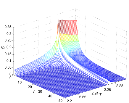
Figure 1: (color online) The correlation entropy as a function of temperature $T$ (in unit of Ising coupling) and the distance $r$ (in unit of $\sqrt{2}$ lattice constant).

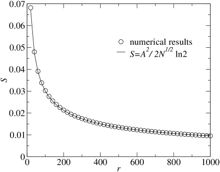
Figure 2: (color online) The correlation entropy as a function of the distance $r$ (in unit of $\sqrt{2}$ lattice constant) at the critical point.

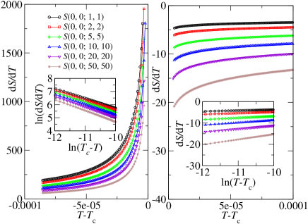
Figure 3: (color online) The critical behavior of the correlation entropy. LEFT: $dS({0,0:N,N})/dT$ below $T_{c}$, and the inset is to explore its critical exponent. RIGHT: $dS({0,0:N,N})/dT$ above $T_{c}$.

The result is impressive. It is well known that the two-dimensional Ising model has two different phases separated by $T_{c}$. Below $T_{c}$, the system has macroscopic magnetization, i.e., spontaneously magnetized, and its mean magnetization is determined by Eq. (54). While above $T_{c}$, the thermal fluctuation destroy this order and the system becomes paramagnetic. Therefore, it is not difficult to understand that the correlation entropy between two sites decay quickly as the distance increases. This fact implies that the extensive property of the entropy holds beyond a finite correlation length. So the physics in a small system can be used to described that for a large system. It is also the reason why in the Monte Carlo approach, a simulation on a small system at low temperature and higher temperature agree with the analytic result in thermodynamic limit excellently. However, in the critical region, as we can see from Fig. 1, the correlation entropy decays in a power-law way. This fact not only tells us a strong dependence between arbitrary two sites in the system, but also manifests the integrality of the whole system. It is also the reason of the difficulty of the Monte-Carlo simulation around the critical region.

Moreover, since the correlation entropy comprises all kinds of two-point correlation function in its expression, it can tell us more details about the critical phenomena. At the critical point, $S({\bf i})=1$ because of $\langle\sigma^{z}_{\bf i}\rangle=0$, and the correlation function behaviors like

$$S_{N}\equiv\langle\sigma_{0,0}^{z}\sigma_{N,N}^{z}\rangle\simeq A/N^{1/4},$$ (63)

where $A\simeq 0.645$. Then the two-site entropy can be simplified as

$$S({\bf ij}) = 2-\frac{1}{2}\left[(1+S_{N})\log_{2}(1+S_{N})\right.$$ (64)

$$\left.+(1-S_{N})\log_{2}(1-S_{N})\right],$$

in the large $N$ limit, and the correlation entropy behaviors like

$$S(0,0:N,N)=\frac{A^{2}}{2N^{1/2}\ln 2},$$ (65)

as has been shown in Fig. 2. On the other hand, around the critical point, the correlation entropy can be written as

$$S({\bf i:j})\simeq\frac{1}{2}\langle\sigma^{z}_{\bf i}\sigma^{z}_{\bf j}\rangle^{2}-\langle\sigma^{z}_{\bf i}\sigma^{z}_{\bf j}\rangle\langle\sigma^{z}_{\bf i}\rangle^{2}$$ (66)

Then

$$\frac{\partial S({\bf i:j})}{\partial T} = \left[\langle\sigma^{z}_{\bf i}\sigma^{z}_{\bf j}\rangle-\langle\sigma^{z}_{\bf i}\rangle^{2}\right]\frac{\partial\langle\sigma^{z}_{\bf i}\sigma^{z}_{\bf j}\rangle}{\partial T}$$ (67)

$$-2\langle\sigma^{z}_{\bf i}\sigma^{z}_{\bf j}\rangle\langle\sigma^{z}_{\bf i}\rangle\frac{\partial\langle\sigma^{z}_{\bf i}\rangle}{\partial T}$$

Therefore, in the critical region below $T_{c}$, the dominant term in $\partial S({\bf i,j})/\partial T$ is $2\langle\sigma^{z}_{\bf i}\sigma^{z}_{\bf j}\rangle\langle\sigma^{z}_{\bf i}\rangle{\partial\langle\sigma_{\bf i}\rangle}/{\partial T}$, which leads to that $\partial S({\bf i,j})/\partial T$ diverges as $T\rightarrow T_{c}$, and scales like

$$\frac{\partial S({\bf i:j})}{\partial T}\propto|T-T_{c}|^{-3/4},$$ (68)

as we can see from the left picture in Fig. 3. Then the critical exponents of $\partial S({\bf i,j})/\partial T$ below $T_{c}$ is 3/4, which is consistent with the critical exponent 1/8 of $\langle\sigma_{\bf i}\rangle$. While in the critical region above $T_{c}$, $\langle\sigma^{z}_{\bf i}\rangle$ vanishes and the dominating term in $S({\bf i:j})$ becomes the correlation function. Then $\partial S({\bf i,j})/\partial T$ scales like

$$\frac{\partial S({\bf i:j})}{\partial T}\propto\ln|T-T_{c}|,$$ (69)

which is the same as the specific heat $C_{v}$. Therefore, the critical exponent now becomes 0 (See the right picture in Fig. 2 ). Moreover, we also note that the slope of lines in the right inset of Fig. 2 is not the same. This is due to the fact that the exponent of the correlation function $\nu$ introduce the distance dependence in the $\partial S({\bf i:j})/\partial T$ above $T_{c}$.

V Quantum phase transition: one-dimensional transverse field Ising model

We now study the correlation entropy in one-dimensional transverse field Ising model whose Hamiltonian reads

$$H_{\rm Ising}=-\sum_{j=1}^{N}\left[\lambda\sigma_{j}^{x}\,\sigma_{j+1}^{x}+\sigma_{j}^{z}\right],$$

$$\sigma_{1}=\sigma_{N+1}$$ (70)

where $\lambda$ is an Ising coupling in unit of the transverse field. The Hamiltonian changes the number of down spins by two, the total space of system then can be divided by the parity of the number of down spins. That is the Hamiltonian and the parity operator $P=\prod_{j}\sigma_{j}^{z}$ can be simultaneously diagonalized and the eigenvalues of $P$ is $\pm 1$. We confine our interesting to the correlation entropy between two spins at position $i$ and $j$ in the chain. Therefore we need to consider both single-site reduced density matrix $\rho_{i}$ obtained from the ground-state wave function by tracing out all spins except the one at site $i$, and the two-site reduced density matrix $\rho_{ij}$ obtained by tracing out all spins except those at site $i$ and $j$. Then if there is no symmetry broken, such as in a finite-size system, according to the parity conservation, $\rho_{i}$ has a diagonal form Eq. (51), and the reduced density matrix of two spins on a pair of lattice sites $i$ and $j$ can be put into the following block-diagonal form

$${\rho}_{ij}=\left(\begin{array}[]{llll}u^{+}&0&0&z^{-}\\ 0&w_{1}&z^{+}&0\\ 0&z^{+}&w_{2}&0\\ z^{-}&0&0&u^{-}\end{array}\right)$$ (71)

in the basis $|\uparrow\uparrow\rangle,|\uparrow\downarrow\rangle,|\downarrow\uparrow\rangle,|\downarrow\downarrow\rangle$. The elements in the density matrix $\rho_{ij}$ can be calculated from the correlation function.

$$u^{\pm}=\frac{1}{4}(1\pm 2\langle\sigma_{i}^{z}\rangle+\langle\sigma_{i}^{z}\sigma_{j}^{z}\rangle),$$

$$w_{1}=w_{2}=\frac{1}{4}(1-\langle\sigma_{i}^{z}\sigma_{j}^{z}\rangle),$$

$$z^{\pm}=\frac{1}{4}(\langle\sigma_{i}^{x}\sigma_{j}^{x}\rangle\pm\langle\sigma_{i}^{y}\sigma_{j}^{y}\rangle)$$ (72)

Otherwise, if the symmetry is broken at the ground state of the ordered phase in the thermodynamic limit, i.e. $\langle\sigma^{x}\rangle\neq 0$, then the single-site reduced density matrix becomes

$${\rho}_{i}=\frac{1}{2}\left(\begin{array}[]{cc}1+\langle\sigma^{z}_{i}\rangle&\langle\sigma_{i}^{x}\rangle\\ \langle\sigma_{i}^{x}\rangle&1-\langle\sigma^{z}_{i}\rangle\\ \end{array}\right),$$ (75)

and the two-site reduced density matrix return to the original form (22) since no symmetry can be used to simply it. Therefore, the correlation entropy between two sites $i$ and $j$ becomes

$$S(i:j)=2{\rm tr}\rho_{i}\log_{2}\rho_{i}-{\rm tr}\rho_{ij}\log_{2}\rho_{ij}.$$ (76)

Taking into account the translation invariance, the correlation entropy is simply a function of the distance between two sites.

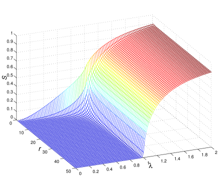
Figure 4: (color online) The correlation entropy as a function of $\lambda$ and the distance $r$ (in unit of lattice constant) at $T=0$ for a system with $N=5000$.

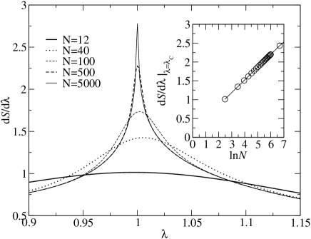
Figure 5: The scaling behavior the correlation entropy between two neighboring sites.

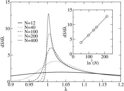
Figure 6: The scaling behavior the correlation entropy between two sites at the longest distance.

The transverse field Ising model can be solved exactly in terms of Jordan-Wigner transformation. The mean magnetization is given by EBarouch70

$$\langle\sigma^{z}\rangle=\frac{1}{N}\sum_{\phi}\frac{(1-\lambda\cos\phi)\tanh[\omega_{\phi}/T]}{\omega_{\phi}},$$ (77)

where $\omega_{\phi}$ is the dispersion relation,

$$\omega_{\phi}=\sqrt{1+\lambda^{2}-2\lambda\cos(\phi_{q})},$$

$$\phi_{q}=2\pi q/N,$$ (78)

where $q$ is integer (half-odd integer) for parity $P=-1(+1)$. The two-point correlation functions are calculated as EBarouch71

$$\langle\sigma_{0}^{x}\sigma_{N}^{x}\rangle=\left|\begin{array}[]{cccc}a_{-1}&a_{-2}&\cdots&a_{-N}\\ a_{0}&a_{-1}&\cdots&a_{-N+1}\\ \vdots&\vdots&\vdots&\vdots\\ a_{N-2}&a_{N-3}&\cdots&a_{-1}\end{array}\right|$$ (83)

$$\langle\sigma_{0}^{y}\sigma_{N}^{y}\rangle=\left|\begin{array}[]{cccc}a_{1}&a_{0}&\cdots&a_{-N+2}\\ a_{2}&a_{1}&\cdots&a_{-N+3}\\ \vdots&\vdots&\vdots&\vdots\\ a_{N}&a_{N-1}&\cdots&a_{1}\end{array}\right|$$ (88)

$$\langle\sigma_{0}^{z}\sigma_{N}^{z}\rangle=4\langle\sigma^{z}\rangle^{2}-a_{N}a_{-N}$$ (89)

where

$$a_{N}=\frac{1}{N}\sum_{\phi}\frac{\cos(\phi N)(\lambda\cos\phi-1)\tanh[\omega_{\phi}/T]}{\omega_{\phi}}$$

$$-\frac{\lambda}{N}\sum_{\phi}\frac{\sin(\phi N)\sin(\phi)\tanh[\omega_{\phi}/T]}{\omega_{\phi}}$$ (90)

We show the correlation entropy $S(i:j)$ in the ground state as a function of coupling $\lambda$ and distance between two site $r=i-j$ in Fig. 4. The result is also impressive. As is well known Sachdev , the ground state of the transverse field Ising model consists of two different phases, whose corresponding physical picture can be understood from both weak and strong coupling limit. If $\lambda\rightarrow 0$, all spins are polarized along $z$ direction, the ground state then is a paramagnet and in the absence of long-range correlation, while in the limit $\lambda\gg 1$, the strong Ising coupling introduce magnetic long-range correlation in the order parameter $\sigma^{x}$ to the ground state. The competition between these two different order leads to a quantum phase transition at the critical point $\lambda_{c}=1$. From Fig. 4, we can see that the correlation entropy tends to zero quickly as the distance between two sites increases in the paramagnetic phase. This phenomena can be well understood from the fact that the ground state in this phase is non-degenerate and almost fully polarized, therefore the knowledge of the state at one site $i$ does not effect the state of another site $j$ far away, which leads to zero information in common between two sites. However, this scene is not true in another phase. When $\lambda>1$, the ground state is twofold degenerate and possess long-range correlation. Before the measurement, the uncertainty of the state at an arbitrary site is very large. However, if we learn it from one site, the state at another site, even far away, is almost determined. Which leads to a finite correlation entropy between two sites even if they are separated far away from each other.

Obviously, the behavior of correlation entropy in the transverse field Ising model is quite different from the quantum entanglement. In the previous works AOsterloh2002 ; TJOsbornee on the pairwise entanglement in the ground state of this model, it has been shown that the concurrence vanishes unless the two sites are at most next-nearest neighbors. In the paramagnetic phase, the correlation entropy share similar properties in common with the concurrence. In the ordered phase, however, the correlation entropy does not vanish even the distance between two sites becomes very large, such as 50 lattice constant. Moreover, the correlation entropy also shows interesting scaling behavior, just as that of the concurrence, around the critical point, as is shown in Fig. 5. Moreover, we find that at the critical point the first derivative of the correlation entropy between two neighboring sites scales like

$$\left.\frac{dS(0,1)}{d\lambda}\right|_{\lambda=\lambda_{c}}\simeq{\rm const}\times\ln N.$$ (91)

or

$$S(0,1)\simeq S(0,1)|_{\lambda=\lambda_{c}}+{\rm const}\times(\lambda-\lambda_{c})\ln N.$$ (92)

However, for those sites are separated far away, the correlation entropy shows quite different scaling behavior. For examples, in Fig. 6, we show the scaling behavior the correlation entropy between two sites at the longest distance in a ring. This first observation is that when $N\rightarrow\infty$, ${dS(0,N/2)}/{d\lambda}$ becomes divergent. Moreover, detailed analysis reveal that the maximum value of the first derivative of the correlation entropy between two farthest sites in a ring scales like

$$\frac{dS(0,N/2)}{d\lambda}\simeq{\rm const}\times\ln^{3}N.$$ (93)

which differs from $\ln N$ for ${dS(0,1)}/{d\lambda}$. Obviously, these interesting scaling behavior enable us to learn the physics of real infinite system from the scaling analysis.

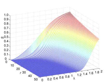
Figure 7: (color online) The correlation entropy as a function of $\lambda$ and the distance $r$ (in unit of lattice constant) at $T=0.2$. Obviously, at low temperature, the correlation entropy at long distance is destroyed in the quantum critical region around $\lambda=1$.

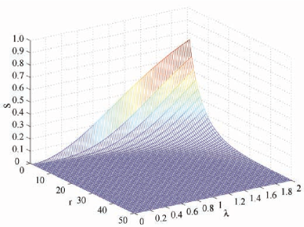
Figure 8: (color online) The correlation entropy as a function of $\lambda$ and the distance $r$ (in unit of lattice constant) at $T=0.5T$. At higher temperature, the correlation entropy at long distance is completely destroyed.

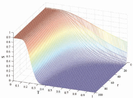
Figure 9: (color online) The correlation entropy as a function of temperature $T$ and the distance $r$ (in unit of lattice constant) at $\lambda=2.0$. We can see from the figure that the correlation entropy is protected by an energy gap at low temperature.

On the other hand, there is no thermal phase transition in one-dimensional quantum spin system according to the Mermin-Wagner theorem NDMermin66 . Thus let us study the properties of the correlation entropy away from zero temperature. The results are shown in Fig. 7 and 8 for $T=0.2$ and $0.5$ respectively. We can see that at lower temperature $T=0.2$, the correlation entropy is broken only around the critical region $\lambda\sim 1$. As the temperature increases, the correlation entropy in larger $\lambda$ region is also destroyed. These observations tell us that the correlation entropy is a decreasing function of the temperature, as we can see from Fig. 9. Since the broken symmetry only exists in the ground state of an infinite system and the thermal fluctuation tends to destroy the correlation entropy, it is not possible to reestablish such a long-range correlation at finite temperatures. Therefore, no thermal phase transition happens in the one-dimensional transverse field Ising model. This observation, based on the numerical calculation, is consistent with the Mermin-Wagner theorem.

VI discussions and prospects

With analytical studies and numerical calculations, we have discovered the rigorous relation between the correlation entropy and the long-range correlation. It strongly indicates us the non-trivial role of the correlation entropy in the critical phenomena. This discovery motivates us to study both the thermal and quantum phase transitions from the point view of information theory, i.e. mutual information, whose non-vanishing behavior at long distance really witnesses the violation of the extensive properties of the entropy in the statistical physics, i.e. $S($AB$)=S($A$)+S($B$)$. In the two models we studied in this model, since the correlation length at the critical point diverges, the physics of the system has a strong dependence on the system size, i.e. the scaling behavior. On the other hand, it also implies that the entropy at the critical point is no longer a linear function of the volume of the system, i.e. $S\neq sV$. In one dimensional system, it has already been noted that entropy of the subsystem satisfies $S(x)\propto\ln(x)$ korepin2004 where $x$ is the length of subsystem in the critical region of some spin systems. Then, from this point of view, the spatial degree of freedom of the system is suppressed around the critical point. This observation reminds us a well-known holographic principle on the entropy of the black hole which says that the entropy of the black hole is proportional to the surface. Though a rigorous prove is still not available, we are sure there there are something in common between the entropy in the critical phenomena and that in the black hole, and this relation deserve for further investigation.

On the other hand, though we restrict ourselves to the two-point correlation entropy in the above studies, if the system processes block-block order, such as dimer order CKMajumdar69 , it may be useful to investigate the properties of block-block correlation entropy. A simple example is Majumdar-Ghosh model with the Hamiltonian ${H}=\sum_{i}\left(J_{1}{\bf\sigma}_{i}\cdot{\bf\sigma}_{i+1}+J_{2}{\bf\sigma}_{i}\cdot{\bf\sigma}_{i+2}\right)$, where $J_{2}$ is the coupling between two next-nearest neighbor sites. In this model, if $J_{2}=1/2$, the ground state is a uniformly weighted superposition of the two nearest-neighbor valence bond state CKMajumdar69 :

$$|\psi_{1}\rangle=[1,2][3,4]\cdots[L-1,L]$$

$$|\psi_{2}\rangle=[L,1][2,3]\cdots[L-2,L-1]$$ (94)

where

$$[i,j]=\frac{1}{\sqrt{2}}(|\uparrow\rangle_{i}|\downarrow\rangle_{j}-|\downarrow\rangle_{i}|\uparrow\rangle_{j}).$$ (95)

Then the block-block correlation entropy can help us to understand such a dimer order.

Moreover, from the definition of our correlation entropy, it is also useful to introduce a characteristic length for the statistical system, below which the extensive properties of the entropy is violated. Such a characteristic length has a non-trivial meaning, since the extensive property of the entropy in the statistical physics is only valid above this scale. A simple example is the molecule which is composed of some atoms. When we study the physics of molecule gas, we have to regard a molecule as a whole because of its internal order. Only when the temperature is high enough to break its order, the atom then plays the important role to the statistical properties of the system.

Though we verify the non-trivial behavior of the correlation entropy in terms of spin systems, the rigorous relation between the non-vanishing correlation entropy and long-rang correlation is valid for all many-body systems. Therefore, it is expected to provide more physical intuition into the critical phenomena, such as Bose-Einstein condensation and superconductivity from the point view of the correlation entropy. Take the former as a simple example, the reduced density matrix between two sites in the space-time can also be expressed in terms of bosons operators $a_{\bf x,p}^{\dagger}|0\rangle=\exp(-i{\bf px})$ in space representation. At high temperatures, $\langle{\bf p}|\rho_{\bf xx^{\prime}}|{\bf p^{\prime}}\rangle$ vanishes as ${\bf x-x^{\prime}}$ increases. Only when the condensation happens, $\langle{\bf 0}|\rho_{\bf xx^{\prime}}|{\bf 0}\rangle$ leads to a non-vanishing correlation entropy, just as what we have shown for the correlation entropy in quantum spin system.

VII Summary and acknowledgement

In summary, the correlation entropy plays a universal role in understanding critical phenomena. Its non-vanishing behavior not only help us have deep understanding to the entropy in the statistical physics, but also shed light on the long-range correlation in the critical behavior.

This work is supported by the Earmarked Grant for Research from the Research Grants Council of HKSAR, China (Project CUHK N_CUHK204/05 and HKU_3/05C) and UGC of CUHK; and NSFC with Grants No. 90203018, No. 10474104 and No. 60433050. We thank Kerson Huang for the helpful discussion.

References

- (1) K. Huang, Statistical mechanics, (Wiley, New York, 1987).
- (2) C. E. Shannon, A mathematical theory of communication, Bell System Tech. J., 27, pp. 379-423 and 623-656, 1948.
- (3) T. M. Cover and J. A. Thomas, Elements of information theory, (John Wiley and Sons, New York, 1991).
- (4) M. A. Nilesen and I. L. Chuang, Quantum Computation and Quantum Information (Cambridge University Press, Cambridge, England, 2000)
- (5) A. Wehrl, Rev. Mod. Phys. 50, 221 (1978).
- (6) V. Vedral and M. B. Plenio, Phys. Rev. Lett. 78, 2275 (1997).
- (7) R. Shankar, Rev. Mod. Phys. 66, 129 (1994).
- (8) D. P. Landau, K. Binder, A Guide to Monte Carlo Simulations in Statistical Physics, (Cambridge Univ Press, 2006)
- (9) S. Sachdev, Quantum Phase Transitions, (Cambridge University Press, Cambridge, UK, 2000).
- (10) A. Osterloh, Luigi Amico, G. Falci and Rosario Fazio, Nature 416, 608 (2002).
- (11) T. J. Osborne and M.A. Nielsen, Phys. Rev. A 66, 032110(2002).
- (12) S. J. Gu, H. Q. Lin, and Y. Q. Li, Phys. Rev. A 68, 042330 (2003); S. J. Gu, G. S. Tian, H. Q. Lin, Phys. Rev. A 71, 052322 (2005).
- (13) S. J. Gu, S. S. Deng, Y. Q. Li, H. Q. Lin, Phys. Rev. Lett. 93, 086402 (2004).
- (14) A. Anfossi, P. Giorda, A. Montorsi, and F. Traversa, Phys. Rev. Lett. 95, 056402 (2005).
- (15) H. T. Quan, Z. Song, X. F. Liu, P. Zanardi, and C. P. Sun, Phys. Rev. Lett. 96, 140604 (2006).
- (16) P. Jordan, Z. Phys. 94, 531 (1935); J. Schwinger, in Quantum Theory of Angular Momentum, edited by L. C. Biedenharn and H. Van Dam (Academic, New York, 1965).
- (17) V. Vedral, Rev. Mod. Phys. 74, 197 (2002).
- (18) O. Klein, Z. Phys. 72, 767 (1931).
- (19) C. N. Yang, Rev. Mod. Phys. 34, 694 (1962).
- (20) W. Kohn and D. Sherrington, Rev. Mod. Phys. 42, 1 (1970).
- (21) Those quantum phase transitions induced by the ground-state level-crossing in a small system are not included.
- (22) L. Onsager, Phys. Rev. 65, 117 (1944).
- (23) B. M. Mccoy, and T. T. Wu, The Two-dimensional Ising Model, (Harvard University Press, Cambridge, Massachusetts, 1973).
- (24) E. Barouch and B. M. McCoy, Phys. Rev. A 2, 1075 (1970).
- (25) E. Barouch and B. M. McCoy, Phys. Rev. A 3, 786 (1971).
- (26) N. D. Mermin and H. Wagner, Phys. Rev. Lett. 17, 1133 (1966).
- (27) C.K. Majumdar and D.K. Ghosh, J. Math. Phys. 10, 1388 (1969).
- (28) V. E. Korepin, Phys. Rev. Lett. 92, 096402 (2004).