Robust transmission of non-Gaussian entanglement over optical fibers

Abstract

We show how the entanglement in a wide range of continuous variable non-Gaussian states can be preserved against decoherence for long-range quantum communication through an optical fiber. We apply protection via decoherence-free subspaces and quantum dynamical decoupling to this end. The latter is implemented by inserting phase shifters at regular intervals $\Delta$ inside the fiber, where $\Delta$ is roughly the ratio of the speed of light in the fiber to the bath high-frequency cutoff. Detailed estimates of relevant parameters are provided using the boson-boson model of system-bath interaction for silica fibers, and $\Delta$ is found to be on the order of a millimeter.

I Introduction

Gaussian entangled states of two subsystems are well studied in the quantum communication and information literature. These states are often encountered in quantum communication experiments. However non-Gaussian entangled states are also important in the context of quantum communication. For example, such a communication system may be constructed in two steps geo : (a) encoding based on product states of Gaussian states, (b) decoding based on measurement on this continuous set of Gaussian states. During decoding, one must generate superpositions of input Gaussian states, which are essentially non-Gaussian states. Thus quantum communication systems may require non-Gaussian states. Moreover, it is impossible to achieve a quantum speed-up using only harmonic oscillators and corresponding Gaussian operations bartlett : the dynamics of such a system can be efficiently simulated classically. This, in turn, means that to gain a quantum advantage in this scenario, one needs to use non-Gaussian operations. It has also been shown that the distillation of entanglement from two Gaussian entangled states is impossible using only local Gaussian operations and classical communication eisert . Thus, both quantum speed-up and distillation of entanglement, which have a close relationship with quantum error correction, require non-Gaussian operations. Recently there have been a few proposals to detect entanglement in such non-Gaussian states biswas ; vogel ; hillery .

In this work we focus on the problem of preserving non-Gaussian entanglement in noisy quantum communication channels. There have been several proposals based on quantum purification protocols and quantum repeaters to communicate entangled photonic qubits over long distances bennett ; deutsch ; dur . Alternatively, entanglement between distant nodes can be prepared by measurements along a chain of intermediate particles WuLidarSchneider:04 ; Compagno:04 . The problem we address here is quite different: rather than setting up remote entanglement between distant nodes, we consider the problem of transmitting entangled field states for a long distance along an optical fiber. Specifically, we propose a method that preserves the multiphoton entanglement of a class of non-Gaussian states transmitted through an optical fiber. Most optical fibers are known to have minimum loss windows at wavelengths of the order of few microns. The optical frequencies generally suffer attenuation inside such a fiber. This loss adds to other decoherence processes which degrade the fidelity of entanglement transmission. We propose a hybrid approach to control decoherence of optical-frequency non-Gaussian states inside an optical fiber. Specifically, we utilize decoherence-free subspace (DFS) dfs and quantum dynamical bang-bang (BB) decoupling BB protection to preserve non-Gaussian entanglement. The DFS protection is used against differential dephasing of the two field modes used to construct non-Gaussian entangled states. The BB process is applied in order to deal with the remaining relevant decoherence sources, in particular Raman scattering. This is done by inserting phase shifters at regular intervals along the length of the optical fiber, similarly to the proposal in lidar where this spatial BB procedure was used to protect single photon polarization states transmitted through optical fibers. In this manner we provide a novel application of the general hybrid DFS-BB strategy proposed in byrd_lidar (see also LidarWu-ERD ).

The structure of the paper is as follows. In Sec. II, we introduce a class of non-Gaussian states and model their interaction with an optical fiber. In Sec. III, we describe in detail a hybrid approach to eliminating their decoherence during transmission through an optical fiber. In Sec. IV, we provide a numerical estimate of loss of entanglement through a realistic fiber using a boson-boson model of interaction between the field and the fiber.

II Interaction mechanism of non-Gaussian entangled states with fiber

II.1 A class of two-mode non-Gaussian states and their entanglement

The simplest examples of non-Gaussian states of the electromagnetic field are the single photon states. Other examples are states generated by excitations of a Gaussian state tara_thermal ; gsapuri . Another method to produce non-Gaussian states uses state-reduction gsa_qo ; yamamoto ; bellini . A recent experimental proposal discusses how to generate non-Gaussian states by subtracting a photon from each mode of a two-mode squeezed vacuum state grangier . We consider non-Gaussian entangled states $|\psi\rangle$ of two field modes $a$ and $b$ ($a$ and $b$ are bosonic annihilation operators), produced by subtracting $p(>0)$ photons from one of the modes (say, $a$) of a squeezed vacuum state $|\phi\rangle$, given by,

$$|\psi\rangle = a^{p}|\phi\rangle\equiv\frac{1}{P}\sum_{n=0}^{\infty}\sqrt{\frac{(n+p)!}{n!}}\zeta^{n+p}|n,n+p\rangle\;,$$ (1)

$$|\phi\rangle \equiv \sum_{n=0}^{\infty}\zeta^{n}|n,n\rangle,$$ (2)

where $\zeta$ is the complex squeezing parameter and $P$ is the normalization constant. This state is non-Gaussian in the sense that its coordinate representation is a non-Gaussian function of space-coordinates $x$ and $y$, as given by,

$$\psi(x,y)=\frac{\zeta^{p}}{\sqrt{2^{p}\pi}}\sum_{n=0}^{\infty}\frac{(\zeta/2)^{n}}{n!}H_{n}(x)H_{n+p}(y)e^{-(x^{2}+y^{2})/2},$$ (3)

where $H_{n}(x)$ is the $n$th order Hermite polynomial. Note that for $p=0$, the state becomes Gaussian.

The entanglement in this state can be verified by the Peres-Horodecki criterion peres . We find that the density matrix of the state $|\psi\rangle$ under transpose of the $b$ mode transforms into

$$\sigma = \frac{1}{P^{2}}\sum_{n,m=0}^{\infty}\zeta^{n+p}\zeta^{*^{m+p}}\sqrt{\frac{(n+p)!(m+p)!}{n!m!}}$$ (4)

$$|n,m+p\rangle\langle m,n+p|\;.$$

The eigenvalues of the above matrix can be calculated as

$$\lambda_{nn} = \frac{1}{P^{2}}|\zeta|^{2(n+p)}\frac{(n+p)!}{n!}\;\;\;\forall n\;,$$

$$\lambda_{nm} = \pm\frac{1}{P^{2}}|\zeta|^{n+m+2p}\sqrt{\frac{(n+p)!(m+p)!}{n!m!}}\;\;\;\forall n\neq m\;.$$

Existence of negative eigenvalues of the matrix $\sigma$ reflects that the state $|\psi\rangle$ is entangled. The negativity $\mathcal{N}$ vidal of the state $|\psi\rangle$ can be written as

$$\mathcal{N}=\frac{1}{P^{2}}\sum_{n=0}^{\infty}\sum_{m\neq n}^{\infty}|\zeta|^{n+m+2p}\sqrt{\frac{(n+p)!(m+p)!}{n!m!}}\;,$$ (6)

which is the absolute sum of all negative eigenvalues of the density matrix $\sigma$. The non-zero value of $\mathcal{N}$ reflects that the state is entangled. Deviation of the value of $\mathcal{N}$ from zero is a measure of the degree of entanglement. It is thus clear from Fig. 1 that the two modes become more entangled with increasing values of $|\zeta|$.

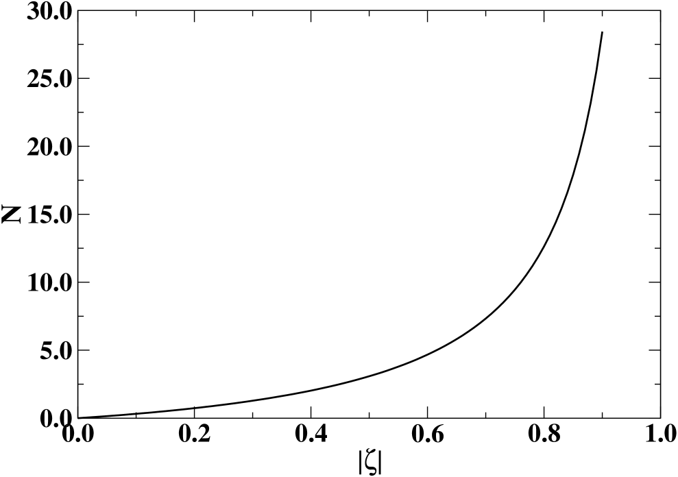
Figure 1: Variation of negativity $\mathcal{N}$ with the squeezing parameter $|\zeta|$ for $p=1$.

II.2 Model of interaction with an optical fiber

We assume that the state $|\psi\rangle$ is transmitted through an optical fiber of length $L$ and thereby interacts with the fiber modes, which leads to decoherence of the state. An optical fiber consists of many dielectric molecules, each of which contains many electronic energy levels. The interaction of the input field states with the fiber can be reasonably described by a molecule-field interaction Hamiltonian. Dominant decoherence mechanisms are phase damping and energy exchange between the field and the molecules.

The exchange processes can be expressed via the following Hamiltonian, under the rotating-wave approximation:

$$H_{I}\equiv\sum_{i}(A_{i}^{{\dagger}}B_{i}+\mathrm{h.c.}),$$ (7)

where $A_{i}$ describes the field operators and $B_{i}$ describes the molecular operators. Here the molecules in the fiber act as the bath, leading to decoherence.

The exact form of the field operators $A_{i}$ in the above Hamiltonian depends upon the model of the interaction. For example, if the field modes are at near-resonance with the single-photon transition in the molecules, dipole coupling between them leads to $A_{i}\equiv a,b$. Dipole coupling dominates higher order coupling (e.g., quadrupole coupling or magnetic dipole coupling), which would lead to multi-photon processes. Thus, at near-resonance, single-photon absorption by the molecules leads to decoherence. Clearly, far from single-photon resonance, higher order processes can dominate. In light of these considerations, we assume that the frequencies of the two field modes are so chosen that two-photon processes may occur in the system, while the cross-section of single-photon processes becomes negligible. Specifically, we choose the frequencies of the field-modes to be much smaller than the energy gaps between the ground and first excited electronic states.

There are two different kinds of two-photon processes that may occur in a molecule: annihilation (creation) of two photons described by $a^{2}$, $b^{2}$, and $ab$ ($a^{{\dagger}2}$, $b^{{\dagger}2}$, and $a^{{\dagger}}b^{{\dagger}}$), and photon-number conserving processes (described by $a^{{\dagger}}b$, $ab^{{\dagger}}$, $a^{{\dagger}}a$, and $b^{{\dagger}}b$). If we assume the molecules are in their electronic ground states (at low temperature, as discussed later), the process of absorption of two photons of two orthogonal modes is disallowed due to certain selection rules cohen . Moreover, as both modes propagate in the same direction through the fiber, Doppler shift of the photon frequency causes the absorption processes of two photons in the same mode to be off-resonance cohen . Thus, we are led to a situation where most of the molecular levels are resonant with the second kind of two-photon transitions. This means that low-energy scattering of the photons, namely Raman (described by $a^{{\dagger}}b$ and $ab^{{\dagger}}$) and dephasing processes (described by the number operators $n_{a}\equiv a^{{\dagger}}a$ and $n_{b}\equiv b^{{\dagger}}b$, which is equivalent to Rayleigh scattering), are most likely to occur inside the fiber. In this case, we can write the effective interaction Hamiltonian in the rotating wave approximation as

$$H_{I} = \sum_{i}g_{i}(a^{{\dagger}}bB_{i}+ab^{{\dagger}}B_{i}^{{\dagger}})+\sum_{i}(\Gamma_{a}^{i}n_{a}+\Gamma_{b}^{i}n_{b})B_{\mathrm{ph}}^{i}\;$$ (8)

$$\equiv H_{I}^{(1)}+H_{I}^{(2)},$$

where $B_{i}$ is the annihilation operator that corresponds to relevant transitions of $i$th molecule in the fiber, $g_{i}$’s are the coupling strengths, $B_{\mathrm{ph}}^{i}$ is the dephasing operator for the $i$th molecule (the exact form of this will be discussed later), and $\Gamma_{a}^{i}$ and $\Gamma_{b}^{i}$ are the respective dephasing rates of the two modes $a$ and $b$.

III A hybrid approach to eliminate decoherence

III.1 A decoherence-free subspace against differential dephasing

In this section we discuss a hybrid approach to suppress these two-photon processes, i.e., how the effect of the interaction Hamiltonian (8) on the state $|\psi\rangle$ can be eliminated. We start with the dephasing processes described by the number operators $n_{a}\equiv a^{{\dagger}}a$ and $n_{b}\equiv b^{{\dagger}}b$. We rewrite the dephasing part of the Hamiltonian (8), $\sum_{i}(\Gamma_{a}^{i}n_{a}+\Gamma_{b}^{i}n_{b})B_{\mathrm{ph}}^{i}$, in terms of two collective operators

$$A_{\pm}=n_{a}\pm n_{b}$$ (9)

as $\sum_{i}(\Gamma_{-}^{i}A_{-}+\Gamma_{+}^{i}A_{+})B_{\mathrm{ph}}^{i}$, where $\Gamma_{\pm}^{i}=(\Gamma_{a}^{i}\pm\Gamma_{b}^{i})/2$. Note that the two-mode number states $|n,n+p\rangle$ and $|n+p,n\rangle$ are eigenstates of the operator $A_{-}=n_{a}-n_{b}$ for all integers $p\geq 0$. Thus these states form manifolds of decoherence-free subspaces with respect to differential dephasing for a given $p$. In any manifold $\{|n,n+p\rangle\}$ ($p$ fixed), any arbitrary superposition of all possible states is also a decoherence-free state dfs . In this way, in the present case the state $|\psi\rangle$ is a DFS under the action of collective dephasing $A_{-}$. Note that this protection does not require encoding, in contrast to the usual construction of decoherence-free subspaces dfs .

III.2 Bang-bang decoupling of the Raman process

As a second layer of protection of the state against other decoherence processes (described by Raman interactions), we now follow the general hybrid DFS-BB method proposed in byrd_lidar . In the standard BB decoupling methods BB , one uses very short pulses so as to cancel the effective interaction Hamiltonian. Thus one ends up with only that component of the total Hamiltonian of system and bath which commutes with the BB pulses. If the pulses are appropriately chosen, entanglement generation between the system and bath states can thus be prevented, and decoherence of the system is prevented. However, one has to apply the pulses in intervals shorter than the timescale of decay of the bath correlation. A recent proposal lidar uses a spatial, rather than temporal version of this idea to overcome decoherence of a single-photon polarization state in optical fibers. Ref. lidar shows how to replace the short time-dependent pulses with phase shifters at regular intervals. Our approach here is similar except that we deal with non-Gaussian entanglement rather than single-photon states, and introduce a hybrid DFS-BB approach. In this way entanglement can be transmitted over a long distance in quantum communication systems.

Let us start with the total system-bath Hamiltonian in the form

$$H = H_{0}+H_{I},\;$$

$$H_{0} = \hbar\omega_{a}n_{a}+\hbar\omega_{b}n_{b}+H_{B},$$ (10)

where $\omega_{a,b}$ are the frequencies of the two field modes, $H_{B}$ is the free Hamiltonian of the molecular bath, and $H_{I}$ is given by Eq. (8). The frequencies $\omega_{a,b}$ are chosen so that they are off-resonant with single-photon transitions, but possibly resonant with Raman transitions in the fiber molecules. Here and below we omit the zero-point energies when writing oscillator Hamiltonians.

The initial state is $\left|\Psi_{0}\right\rangle=|\psi\rangle\left|M\right\rangle$, where $|\psi\rangle$ is the input non-Gaussian entangled state and $\left|M\right\rangle$ is the state of the bath (for simplicity we use a pure-state notation also for the bath; below we consider the effect of the bath’s state more carefully). At the time $\tau_{L}=L/v$ – where $L$ is the length of the fiber, and $v$ is the average speed of light in the fiber – the total wave function is $\left|\Psi(\tau_{L})\right\rangle=U_{\mathrm{f}}(\tau_{L},0)$ $\left|\Psi_{0}\right\rangle$ (the f subscript stands for “free evolution”). Here the exact normal-ordered propagator is $U_{\mathrm{f}}(\tau_{L},0)=\,:\exp[-i\int_{0}^{L}[H_{I}(x)+H_{0}(x)]dx]:$ (in units where $\hbar=1$). Now, let $\tau=\Delta/v$, and let $N=L/\Delta\gg 1$ so that we can expand the propagator as $U_{\mathrm{f}}(\tau_{L},0)\approx e^{-i\overline{H}(N\Delta)\tau}\cdots e^{-i\overline{H}(2\Delta)\tau}e^{-i\overline{H}(\Delta)\tau}$, where

$$\overline{H}(k\Delta) = \frac{1}{\Delta}\int_{(k-1)\Delta}^{k\Delta}[H_{0}(x)+H_{I}(x)]dx$$ (11)

$$\equiv \overline{H_{0}}(k\Delta)+\overline{H_{I}}(k\Delta)$$

is the average Hamiltonian over the $k$th segment. I.e., we have neglected deviations from average fiber homogeneity, $\delta_{k}=\langle(H(k\Delta)-[H_{I}(k\Delta)+H_{0}(k\Delta)])^{2}\rangle$ (we discuss such deviations in Section IV). The spatial dependence of $H_{0}$ can come from the bath self-Hamiltonian $H_{B}$, while that of $H_{I}$ can come from the coefficients $g_{i}$ and $\Gamma_{a,b}^{i}$ [Eq. (8)]. Therefore:

$$\overline{H_{0}}(k\Delta) = \hbar\omega_{a}n_{a}+\hbar\omega_{b}n_{b}+\overline{H_{B}}(k\Delta)$$

$$\overline{H_{I}}(k\Delta) = \sum_{i}\overline{g_{i}}(a^{{\dagger}}bB_{i}+ab^{{\dagger}}B_{i}^{{\dagger}})$$ (12)

$$+\sum_{i}(\overline{\Gamma_{a}}n_{a}+\overline{\Gamma_{b}}n_{b})B_{\mathrm{ph}}^{i}$$

$$\equiv \overline{H_{I}^{(1)}}(k\Delta)+\overline{H_{I}^{(2)}}(k\Delta).$$

Moreover, in subsection III.3 below we argue that $H_{B}$ is effectively a molecular oscillator Hamiltonian, so that $\overline{H_{B}}(k\Delta)=\sum_{s}\hbar\overline{\Omega_{s}}s$, where $\overline{\Omega_{s}}=\frac{1}{\Delta}\int_{(k-1)\Delta}^{k\Delta}\Omega_{s}(x)dx$ is an average frequency in an $s$-phonon state.

To eliminate the Raman processes dynamically, we propose use of phase shifters, defined by the following operator

$$\Pi=e^{i\pi(n_{a}-n_{b})/2}=\Pi^{{\dagger}},$$ (13)

which generates a relative phase of $\pi$ between the two modes (alternatively we can define $\Pi$ as $e^{i\pi n_{a}}$ or as $e^{i\pi n_{b}}$). When these phase shifters are incorporated inside the fiber at intervals $\Delta$, the Raman interaction part in the Hamiltonian (8) effectively vanishes. This occurs because of the following identities. First, it is simple to show, using the Baker-Campbell-Hausdorff (BCH) formula Reinsch:00 that

$$e^{i\phi n_{a}}a^{\dagger}e^{-i\phi n_{a}}=e^{i\phi}a^{\dagger},\quad e^{i\phi n_{a}}ae^{-i\phi n_{a}}=e^{-i\phi}a,$$ (14)

and similarly for $n_{b}$ and $b$. Therefore

$$\Pi a^{{\dagger}}b\Pi^{{\dagger}} = (e^{i\pi n_{a}/2}a^{\dagger}e^{-i\pi n_{a}/2})(e^{-i\pi n_{b}/2}be^{i\pi n_{b}/2})$$ (15)

$$= -a^{{\dagger}}b\;,$$

$$\Pi ab^{{\dagger}}\Pi^{{\dagger}} = (e^{i\pi n_{a}/2}ae^{-i\pi n_{a}/2})(e^{-i\pi n_{b}/2}b^{{\dagger}}e^{i\pi n_{b}/2})$$ (16)

$$= -ab^{{\dagger}}\;.$$

These identities imply that the Raman interaction is effectively time-reversed every $2\Delta$ due to the action of the phase shifters. To show the utility of this result note first that

$$\Pi\overline{H}\Pi=\overline{H_{0}}-\overline{H_{I}^{(1)}}+\overline{H_{I}^{(2)}},$$ (17)

because the field term of $H_{0}$ and $H_{I}^{(2)}$ obviously commute with $\Pi$ and because averaging commutes with the phase shifter operation. Now, if we install thin phase-shifters inside the fiber at positions $x=0,\Delta,2\Delta,...$, from $A$ to $B$, the evolution will be modified to

$$U(\tau_{L},0)\approx e^{-i\overline{H}(N\Delta)\tau}\cdots\Pi e^{-i\overline{H}(2\Delta)\tau}\Pi e^{-i\overline{H}(\Delta)\tau}\Pi.$$ (18)

Note that in writing this expression we have neglected the variation of $H$ inside the phase-shifter; this will hold provided that the phase-shifter width is much smaller than the distance over which deviations $\delta_{k}$ from average fiber homogeneity become significant. Now assume that the average Hamiltonians over two successive segments are equal:

$$\overline{H_{I}^{(i)}}((k+1)\Delta) = \overline{H_{I}^{(i)}}(k\Delta)\quad i=1,2$$

$$\overline{H_{0}}((k+1)\Delta) = \overline{H_{0}}(k\Delta).$$ (19)

The better this approximation, the better our hybrid DFS-BB method will perform; we address deviations in Section IV. In this case, to first order in $\tau$, and using Eqs. (17) and (18), we have exact cancellation of $H_{I}^{l}$ between successive segments:

$$e^{-i\overline{H}((k+1)\Delta)\tau}\Pi e^{-i\overline{H}(k\Delta)\tau}\Pi$$ (20)

$$= e^{-i\overline{H}((k+1)\Delta)\tau}e^{-i\Pi\overline{H}(k\Delta)\Pi\tau}$$

$$= e^{-i\tau(\overline{H_{0}}(k\Delta)+\overline{H_{I}^{(1)}}(k\Delta)+\overline{H_{I}^{(2)}}(k\Delta))}$$

$$\times e^{-i\tau(\overline{H_{0}}(k\Delta)-\overline{H_{I}^{(1)}}(k\Delta)+\overline{H_{I}^{(2)}}(k\Delta))}$$

$$= e^{-2i(\overline{H_{0}}(k\Delta)+\overline{H_{I}^{(2)}}(k\Delta))\tau},$$

where the smallness of $\tau$ is the justification for adding the arguments of the two exponentials in obtaining the last line. Using Eq. (19) again, this yields the overall evolution operator

$$U(\tau_{L},0)\approx e^{-i\tau_{L}(\overline{H_{0}}(L)+\overline{H_{I}^{(2)}}(L))}.$$ (21)

Thus, to first order in $\tau$ (or the inter-phase shifter distance $\Delta$), we have eliminated the Raman term $\overline{H_{I}^{(1)}}$, and are left with the dephasing term $\overline{H_{I}^{(2)}}=\sum_{i}(\overline{\Gamma_{-}}A_{-}+\overline{\Gamma_{+}}A_{+})B_{\mathrm{ph}}^{i}$, as $\overline{H_{0}}$ causes no decoherence. Considering $\overline{H_{I}^{(2)}}$, we note that the $A_{-}$ component yields only an overall phase on the state $|\psi\rangle$. In fact, the DFS corresponding to $A_{-}$ remains invariant under the action of $\Pi$ as $\Pi$ obviously commutes with $A_{-}$. Therefore, the overall evolution operator reduces to

$$U(\tau_{L},0)\approx e^{-i\tau_{L}(\overline{H_{0}}+\sum_{i}\overline{\Gamma_{+}}A_{+}B_{\mathrm{ph}}^{i})},$$ (22)

(where averages can be considered as being evaluated at $L$) and our remaining task is to eliminate the collective dephasing term (proportional to $A_{+}$). However, it turns out that it is impossible to do this with BB while using only linear optical elements. Fundamentally, the reason for this is that the group generated by $\{n_{a}-n_{b},a^{\dagger}b,b^{\dagger}a\}$ (phase shifters and beam splitters) is non-compact, which means that it can at most apply a dilation but not a sign change, as required for time reversal in the BB protocol. However, as we argue next, the collective dephasing term nevertheless has no significant effect on the preservation of non-Gaussian entanglement.

III.3 Suppression of collective dephasing

In the low temperature limit, most of the molecules in each segment of length $\Delta$ reside in their ground electronic states. In thermal equilibrium, the molecular vibrational states obey Maxwell-Boltzmann statistics. The state of the molecular bath can be well described by a density matrix $\rho_{B}=\sum_{s}p_{s}|\phi_{s}\rangle\langle\phi_{s}|$, where $p_{s}=\exp(-E_{s}/k_{B}T)/Z$ is the Boltzmann probability of an $s$-phonon excitation with energy $E_{s}=\hbar\Omega_{s}$, $k_{B}$ is the Boltzmann constant, and $Z=\sum_{s}\exp(-E_{s}/kT)$ is the partition function, and $|\phi_{s}\rangle$ is the $s$-phonon excited state. This is equivalent to the assumption that the molecular Hamiltonian $H_{B}$ is an oscillator Hamiltonian, i.e., $H_{B}=\sum_{s}\hbar\Omega_{s}s$ ($s$ is the phonon number operator), as mentioned in the previous subsection. Moreover, we assume that the field couples to the molecular vibrations. Then $[H_{B},B_{\mathrm{ph}}^{i}]=0$ and hence $\sum_{i}B_{\mathrm{ph}}^{i}|\phi_{s}\rangle=s|\phi_{s}\rangle$. Under these assumptions we have that $[H_{0},A_{+}B_{\mathrm{ph}}^{i}]=0$, and hence the effect of the pulse operator (22) on the initially uncorrelated system-bath state can be written as

$$\rho_{\mathrm{SB}}(\tau_{L},0) \approx U(\tau_{L},0)(|\psi\rangle\langle\psi|\otimes\rho_{B})U^{{\dagger}}(\tau_{L},0)$$

$$= \sum_{s}p_{s}e^{-i\tau_{L}\overline{H_{0}}}e^{-i\tau_{L}\overline{\Gamma_{+}}sA_{+}}$$

$$\times(|\psi\rangle\langle\psi|\otimes|\phi_{s}\rangle\langle\phi_{s}|)e^{i\tau_{L}\overline{H_{0}}}e^{i\tau_{L}\overline{\Gamma_{+}}sA_{+}}\;.$$

Using the expression (1) for $|\psi\rangle$, we find, after tracing out the bath, that the state of the field modes at the final time $\tau_{L}$ becomes

$$\rho(\tau_{L}) = \frac{1}{P^{2}}\sum_{s}p_{s}\sum_{n,m}\zeta^{n+p}\zeta^{\ast(m+p)}\sqrt{\frac{(n+p)!(m+p)!}{n!m!}}$$

$$\times e^{-i\tau_{L}[\omega_{\mathrm{tot}}+2\Gamma_{+}s](n-m)}|n,n+p\rangle\langle m,m+p|\;,$$

where $\omega_{\mathrm{tot}}=\omega_{a}+\omega_{b}$. The fidelity of this state can be calculated as

$$F(\tau_{L})=\langle\psi|\rho(\tau_{L})|\psi\rangle$$

$$= \frac{1}{P^{4}}\sum_{s}p_{s}\left|\sum_{n}|\zeta|^{2(n+p)}\frac{(n+p)!}{n!}e^{-i\tau_{L}n(\omega_{\mathrm{tot}}+2\Gamma_{+}s)}\right|^{2}\;,$$

which becomes unity if

$$\tau_{L}=l\pi/\{\omega_{\mathrm{tot}}+2\Gamma_{+}s\}\;,$$ (26)

where $l$ is an integer. In this expression $\tau_{L}$ is, of course a function of the summation variable $s$, while in reality there is only a single $\tau_{L}$. However, we observe that there are two physical limits where this dependence of $\tau_{L}$ on $s$ disappears. Namely, if $\omega_{\mathrm{tot}}\ll\Gamma_{+}$ then for $l=s$ we find that $\tau$ becomes $s$-independent. In the opposite limit of very weak collective dephasing we also find that $\tau$ is $s$-independent (there is a physical upper limit on $s$ in the Gibbs state $\rho_{B}=\sum_{s}p_{s}|\phi_{s}\rangle\langle\phi_{s}|$). Both limits can be realized by controlling the field modes $\omega_{a,b}$. Alternatively, in the low temperature limit the sum over $s$ in Eq. (III.3) is dominated by the vibrational ground state, and again the fidelity is unity if $\tau=l\pi/\omega_{\mathrm{tot}}$.

While the fidelity is generally reduced and recovers its initial value of unity only under certain conditions, we next show that the non-Gaussian entanglement can be preserved provided one knows the value of $\Gamma_{+}$. At the exit end of the fiber, the state of the two modes is given by $\rho(\tau_{L},0)$ [Eq. (III.3)]. Taking the partial transpose over the mode $b$ in this state, we obtain:

$$\rho(\tau_{L})^{\mathrm{T_{b}}} = \frac{1}{P^{2}}\sum_{s}p_{s}\sum_{n,m}\zeta^{n+p}\zeta^{\ast(m+p)}\sqrt{\frac{(n+p)!(m+p)!}{n!m!}}$$

$$\times e^{-i\tau_{L}[\omega_{\mathrm{tot}}+2\Gamma_{+}s](n-m)}|n,m+p\rangle\langle m,n+p|\;,$$

The eigenvalues of this matrix are given by

$$\lambda_{nn} = \frac{1}{P^{2}}|\zeta|^{2(n+p)}\frac{(n+p)!}{n!}\;\;\;\forall n\;,$$

$$\lambda_{nm} = \pm\frac{1}{P^{2}}v_{nm}(\tau_{L}\Gamma_{+})|\zeta|^{n+m+2p}$$ (28)

$$\times \sqrt{\frac{(n+p)!(m+p)!}{n!m!}}\;\;\;\forall n,m\neq n,$$

where we have defined the phononic visibility factor as

$$v_{nm}(x)\equiv\left|\sum_{s}p_{s}e^{-2ixs(n-m)}\right|.$$ (29)

For a harmonic oscillator bath this factor can be evaluated analytically, using $E_{s}=\hbar\Omega(s+1/2)$:

$$v_{nm}(x) = \frac{1}{Z}e^{-\hbar\Omega/2k_{B}T}\left|\sum_{s=0}^{\infty}e^{-[\hbar\Omega/k_{B}T+2ix(n-m)]s}\right|$$ (30)

$$= \frac{1}{2Z}\left|\frac{1}{\sinh(\hbar\Omega/2k_{B}T+ix(n-m))}\right|,$$

which is an oscillatory function of its argument $x$, with period $\pi/(n-m)$.

The negativity at the fiber’s end becomes:

$$\mathcal{N}=\frac{1}{P^{2}}\sum_{n=0}^{\infty}\sum_{m\neq n}^{\infty}v_{nm}(\tau_{L}\Gamma_{+})|\zeta|^{n+m+2p}\sqrt{\frac{(n+p)!(m+p)!}{n!m!}}\;,$$ (31)

Comparing this expression to Eq. (6), it is apparent that the negativity is reduced due to the phononic visibility factor. The condition for this factor to become unity is:

$$\tau=\pi/\Gamma_{+},$$ (32)

which can be satisfied provided one knows the value of $\Gamma_{+}$. One way to extract this value is, in fact, to apply our bang-bang protocol and to test the fidelity of the state via quantum state tomography (see ByrdLidar:02 for a more general method relating BB to tomography). Also note that in the low temperature limit, where the sum over $s$ involves only a small number of terms, the phononic visibility factor will still be close to unity. On the other hand, it is clear that if neither condition is met ($\tau\neq\pi/\Gamma_{+}$ and high temperature) then the rapidly oscillating terms in the phononic visibility factor will destructively interfere and cause entanglement loss.

Note also that in absence of any BB control, the initial state $|\psi\rangle$ evolves through the interaction Hamiltonian (8). This leads to different combinations of the photon numbers in the two modes due to energy exchange with the molecular bath. Thus the initial entanglement is destroyed at a length scale $\Delta_{c}$, corresponding to the dissipation time-scale $\tau_{c}$ of the molecular bath.

IV Effect of fiber inhomogeneity on decoherence

So far we have assumed that the average Hamiltonians over two successive segments of length $\Delta$ are equal [Eq. (19)]. However, due to inhomogeneity inside the fiber, the average Hamiltonian differs between segments. In this section, we show that this fluctuation of the average Hamiltonian leads to dissipation of the field and thus sets an upper limit to the value of $\Delta$. We follow and improve the method described in Appendix A of lidar .

IV.1 A Gaussian fluctuations model

The inhomogeneity in the fiber may arise due to nonuniform number density of the molecules or slow time-dependence of the fiber properties. In view of this, we modify the assumption of homogeneity to read

$$H((k-1)\Delta)=H(k\Delta)+\delta(H_{B})_{k}+\delta(H_{I})_{k},$$ (33)

where the operator-valued fluctuations $\delta(H_{B})_{k},\delta(H_{I})_{k}$ in the Hamiltonian are independent. Here $\delta(H_{B})_{k}$  is the fluctuation in the bath-only Hamiltonian, and $\delta(H_{I})_{k}$

$$\delta(H_{I})_{k} = \sum_{i}\delta g_{i}^{k}(a^{{\dagger}}bB_{i}+ab^{{\dagger}}B_{i}^{{\dagger}})_{k}$$ (34)

$$+ \epsilon\sum_{i}(\delta\Gamma_{a}^{i}n_{a}+\delta\Gamma_{b}^{i}n_{b})_{k}(B_{\mathrm{ph}}^{i})_{k}$$

is the operator-valued correction to the interaction Hamiltonian in the $k$th segment, where $\delta g_{i}^{k}$ and $\delta(\Gamma_{l}^{i})_{k}$ ($l=a,b$) are the fluctuations in the coupling coefficients in the $k$th segment, and $\epsilon\ll 1$ is a proportionality constant defining the strength of the fluctuations. We assume that $\epsilon\sim\tau$. These fluctuations lead to losses inside the fiber. However, in an amorphous silica fiber, the loss due to Rayleigh scattering (i.e., due to terms containing $n_{a}$ and $n_{b}$) is much greater than the loss due to other mechanisms (e.g., due to Raman scattering, i.e., due to terms containing $a^{{\dagger}}b$ and $ab^{{\dagger}}$) gpa . With this in mind, we neglect the fluctuations in the Raman terms and henceforth consider only the effect of the fluctuations in $(\Gamma_{a,b}^{i})_{k}$. Thus, in the interaction picture with respect to the energy term $H_{0}+\delta H_{B}(t)$, the interaction Hamiltonian corresponding to the fluctuations in the $k$th segment of the fiber can be written as

$$\delta H_{I}(t)=\epsilon\sum_{i}(f_{a}^{i}(t)n_{a}+f_{b}^{i}(t)n_{b})\;,$$ (35)

where $f_{l}^{i}(t)\equiv\delta\Gamma_{l}^{i}(t)B_{\mathrm{ph}}^{i}$ ($l=a,b$) are the operator-valued fluctuations for the $i$th molecule, and we have replaced the $k$-dependence with time-dependence, in the joint limit $\tau\rightarrow 0$ and total number $N$ of segments large, such that $\tau_{L}=N\tau$ is finite. Under the action of this Hamiltonian $\delta H_{I}(t)$, the evolution of the field state can be described, in the Born approximation, by the following equation scully :

$$\dot{\rho}_{F} = -i\mathrm{Tr}_{B}[\delta H_{I}(t),\rho_{F}(0)\otimes\rho_{B}(0)]$$ (36)

$$- \mathrm{Tr}_{B}\int_{0}^{t}[\delta H_{I}(t),[\delta H_{I}(t^{\prime}),\rho_{F}(t^{\prime})\otimes\rho_{B}(0)]],$$

where the terms up to the second order of $\epsilon(\sim\tau)$ have been considered (as $\epsilon\ll 1$). Now note that since $\Delta\ll L$, the number of segments of length $\Delta$ is much larger than unity. In this limit, the fluctuations $f_{l}^{i}(t)$ can be considered as described by Gaussian operators lidar . Then it is reasonable to assume that the two-time correlations of the form $\Gamma(t,t^{\prime})\equiv\left\langle\left(\sum_{i}f_{l}^{i}(t)\sum_{j}f_{l^{\prime}}^{j}(t^{\prime})\right)\right\rangle_{B}$ ($l,l^{\prime}=a,b$) between these fluctuations do not depend on $a,b$ due to the symmetry properties of Gaussian operators, while the mean $\langle\sum_{i}f_{l}^{i}(t)\rangle_{B}$ vanishes. Here $\langle X\rangle_{B}=\mathrm{Tr}_{B}(\rho_{B}(0)X)$ denotes the average of any operator $X$ over the bath. Taking this average over Eq. (36) leads to the vanishing of the term linear in $\delta H_{I}(t)$, while using the expression for $|\psi\rangle$ [Eq. (1)] we obtain from the integral term:

$$\dot{\rho}_{F} = -\frac{4\epsilon^{2}}{P^{2}}\int_{0}^{t}dt^{\prime}\Gamma(t,t^{\prime})\sum_{n,m}\zeta^{n+p}\zeta^{\ast(m+p)}$$

$$\sqrt{\frac{(n+p)!(m+p)!}{n!m!}}(n-m)^{2}|n,n+p\rangle\langle m,m+p|.$$

This can be solved for the matrix elements of $\rho_{F},$ yielding

$$(\rho_{F})_{n,n+p;m,m+p}(\tau_{L}) = \exp[-4\epsilon^{2}(n-m)^{2}\int_{0}^{\tau_{L}}dt\int_{0}^{t}dt^{\prime}$$

$$\Gamma(t,t^{\prime})](\rho_{F})_{n,n+p;m,m+p}(0),$$

where the initial state is

$$(\rho_{F})_{n,n+p;m,m+p}(0)=\frac{1}{P^{2}}\zeta^{n+p}\zeta^{\ast(m+p)}\sqrt{\frac{(n+p)!(m+p)!}{n!m!}}.$$ (39)

Let us assume that the molecular bath is in thermal equilibrium at temperature $T$. If $T\rightarrow 0$, most of the molecules reside in the ground electronic states. However, molecules can be distributed in all the vibronic modes corresponding to the ground states. The degeneracy of these vibronic states can be lifted by phonon absorption due to molecular collisions. In view of this, we treat the molecules as bosons inside a fiber. As implied by our discussion in the previous section, the dephasing operator $\sum_{i}B_{\mathrm{ph}}^{i}$ can be written as $(B^{{\dagger}}B)_{\mathrm{vib}}$, where $(B)_{\mathrm{vib}}$ is the annihilation operator corresponding to these vibronic states. Thus, the interaction of the field modes with the molecules can be described by the so-called independent oscillator (IO) model ford of boson-boson interactions. In this model, each of the oscillators of the passive molecular bath is linearly coupled to the system oscillator. This interaction is governed by two terms: (i) The Gaussian fluctuations $\sum_{i}f_{l}^{i}(t)$ of the bath operators, and (ii) a memory function $\mu(t)$ of the bath operators, that vanishes at negative times. If the correlation between fluctuations at different times vanishes, the interaction reduces to a Markovian process. However, in general, this correlation is a non-trivial function of time and thus corresponds to a non-Markovian process. It can be shown that the symmetric autocorrelation of $\sum_{i}f_{l}^{i}(t)$ satisfies ford :

$$\frac{1}{2}\left\langle\sum_{i}f_{l}^{i}(t)\sum_{j}f_{l^{\prime}}^{j}(t^{\prime})+\sum_{j}f_{l^{\prime}}^{j}(t^{\prime})\sum_{i}f_{l}^{i}(t)\right\rangle$$ (40)

$$= \frac{1}{\pi}\int_{0}^{\infty}\omega\coth\left(\frac{\hbar\omega}{2k_{B}T}\right)\cos[\omega(t-t^{\prime})]$$

$$\;\;\;\;\;\mathrm{Re}[\tilde{\mu}(\omega+i0^{+})]d\omega\;,$$

while correlations of an odd number of factors of $\sum_{i}f_{l}^{i}(t)$ vanish. Here $\tilde{\mu}(z)$ is the Fourier transform of the memory function $\mu(t)$. Due to the Gaussian property of $\sum_{i}f_{l}^{i}(t)$, as discussed before, the above equals $\langle\sum_{i}f_{l}^{i}(t)\sum_{j}f_{l^{\prime}}^{j}(t^{\prime})\rangle$. The memory function is independent of the potential and the properties of the system and only depends upon the coupling strengths of the field operators with the bath. In the IO model, the coupling strength is an even function of the oscillator frequency and is of the form $m_{j}\omega_{j}^{2}$, where $m_{j}$ is the mass of the $j$th oscillator and the $\omega_{j}$ is the frequency of the $j$th oscillator mode. The spectral distribution of the memory function is in the Ohmic class and can be written as

$$\mathrm{Re}[\tilde{\mu}(\omega+i0^{+})]\approx\pi\omega^{2}e^{-\omega/\omega_{c}}\sum_{j}m_{j}\;,$$ (41)

Here $\omega_{c}$ is the cut-off frequency of the molecular bath modes, and is introduced such that for large frequencies, the memory function does not blow up. This is in conformity with the passivity condition of the molecular bath, which also requires that the bath modes must have an infinite spectrum and the memory function must not be a singular function of $\omega$ ford . Thus using Eqs. (40) and (41), we can write the following expression for the rate of dissipation at time $\tau_{L}$:

$$\Gamma(\tau_{L}) = \int_{0}^{\tau_{L}}dt\int_{0}^{t}dt^{\prime}\Gamma(t,t^{\prime})$$

$$= \int_{0}^{\infty}d\omega\omega^{3}e^{-\omega/\omega_{c}}\coth\left[\frac{\hbar\omega}{2k_{B}T}\right]\left\{\frac{2}{\omega^{2}}\sin^{2}\left(\frac{\omega\tau_{L}}{2}\right)\right\}\;,$$

where we have normalized the memory function (41) in units of mass. For low temperature ($T\rightarrow 0$), when the quantum fluctuations dominate the thermal fluctuations, one can find the actual loss figure as

$$\Gamma(\tau_{L})\approx\omega_{c}^{2}\frac{x^{2}(3+x^{2})}{(1+x^{2})^{2}},\;x=\omega_{c}\tau_{L}\;.$$ (43)

Using the results for the unitary evolution (III.3) and the decay of the density matrix elements given by (LABEL:decay_sol), we find the following expression for the density matrix of the field modes at time $\tau_{L}$:

$$\rho(\tau_{L})_{\mathrm{diss}} = \frac{1}{P^{2}}\sum_{s}p_{s}\sum_{n,m}\zeta^{n+p}\zeta^{\ast(m+p)}\sqrt{\frac{(n+p)!(m+p)!}{n!m!}}$$ (44)

$$\times e^{-i\tau_{L}(\omega_{\mathrm{tot}}+2\Gamma_{+}s)(n-m)}e^{-4\epsilon^{2}\Gamma(\tau_{L})(n-m)^{2}}$$

$$\;\;\;|n,n+p\rangle\langle m,m+p|\;.$$

The eigenvalues of the matrix obtained by taking transpose of the $b$ mode in the above density matrix are given by

$$\lambda_{nn} = \frac{1}{P^{2}}|\zeta|^{2(n+p)}\frac{(n+p)!}{n!}\;\;\;\forall n\;,$$

$$\lambda_{nm} = \pm\frac{1}{P^{2}}\left|\sum_{s}p_{s}e^{-2i\tau_{L}\Gamma_{+}s(n-m)}\right||\zeta|^{n+m+2p}$$

$$\times\sqrt{\frac{(n+p)!(m+p)!}{n!m!}}e^{-4\epsilon^{2}\Gamma(\tau_{L})(n-m)^{2}}\;\;\;\forall n,m\neq n\;.$$

Thus in the low temperature limit, we find the following expression for the negativity:

$$\mathcal{N}_{\mathrm{diss}} = \frac{1}{P^{2}}\sum_{n,m\neq n}|\zeta|^{n+m+2p}\sqrt{\frac{(n+p)!(m+p)!}{n!m!}}$$ (46)

$$\times e^{-4\epsilon^{2}\Gamma(\tau_{L})(n-m)^{2}},$$

where $\Gamma(\tau_{L})$ is given by Eq. (43). Clearly the negativity decreases as the field propagates through the fiber. Using the expression (43) for $\Gamma(\tau_{L})$, we find that for $x\gg 1$ (for $\tau_{L}\gg 1/\omega_{c}$, i.e., on a time-scale much larger than the bath correlation time), the negativity does not decrease further and saturates to (46) with $\Gamma(\tau_{L})$ replaced by $\omega_{c}^{2}$. This saturation is due to the fact that $1/\omega_{c}$ is the timescale over which information about the system state spreads in the bath; for times much longer than this the bath is effectively stationary and no more damage to entanglement in the system is possible via the bath. We next extract a distance scale for the phase shifter separations from these considerations.

IV.2 Numerical estimates of the inter phase-shifter distance

The result (43) due to fluctuation given by (34) leads to an estimate of the spatial separation $\Delta$ between two successive phase-shifters. Note that for $n=m$ (i.e., for diagonal terms of the density matrix) this fluctuation does not lead to any dissipation (or loss of entanglement), as is clear from (LABEL:decay_sol). But the larger is $|n-m|$, the higher is this dissipation. In other words, the largest off-diagonal contribution to the negativity comes from the terms with $|n-m|=1$, which therefore are sufficient to give us the desired estimate of $\Delta$. If we allow an error probability $\delta(\tau_{L})$ over the length of the fiber, then a sufficient condition for the present result to be useful is

$$e^{-4\epsilon^{2}\Gamma(\tau_{L})}>1-\delta(\tau_{L})\;.$$ (47)

Rewriting the above using (43), we have

$$\Delta < \left(\frac{v^{2}(1+x^{2})^{2}}{4\omega_{c}^{2}x^{2}(3+x^{2})}\ln[1-\delta(\tau_{L})]^{-1}\right)^{1/2}$$ (48)

$$\overset{x\rightarrow\infty}{\longrightarrow}\frac{v}{2\omega_{c}}\ln[1-\delta(\tau_{L})]^{-1/2},$$

where we have used $\epsilon=\tau$. The limiting value is attainable by fixing $\Delta$ and letting the number of phase shifters $N$ become very large (long fiber), with $\omega_{c}$ given and fixed. This sets an upper bound on the applicable value of $\Delta$, which is essentially the ratio of the speed of light in the fiber to the bath high-frequency cutoff.

In the following, we present a numerical estimate in a realistic situation, e.g., for an optical fiber with an amorphous silica core. The inhomogeneity in silica leads to fluctuation as described above and thus decoheres the input fields.

The Debye temperature $\Theta=\hbar\omega_{c}/k_{B}$ of crystalline silica is 342 K, where $\omega_{c}$ is the maximum phonon frequency (frequency “cut-off”) allowed inside the crystal. Thus, the lifetime $\tau_{c}$ of phonons becomes of the order of $1/\omega_{c}$. On the other hand, in amorphous solids the Debye temperature and the lifetime of phonons are not well defined. However, at low temperatures $T\ll\Theta$, there exist certain empirical relations between them anderson ; reynolds . For example, at $T=0.2$ K, which corresponds to a phonon frequency of $2.62\times 10^{10}$ Hz, the life-time of phonons is of the order of $10^{-10}$ s. We consider this frequency of phonons as maximum frequency $\omega_{c}$ allowed inside the fiber at $T=0.2$K.

It has been shown that long distance distribution of entangled states of two qubits over a noisy quantum channel can be achieved using entanglement purification protocols bennett ; deutsch . These protocols can be improved in terms of the requirement of physical resources as well as the error threshold, if one uses quantum repeaters dur . It has been shown that for an error probability $\sim 0.01$ (which is much larger than the error threshold for fault-tolerant computation using single qubits) inside the communication channel, quantum purification protocols work well, when combined with quantum repeaters. Although, as explained in the introduction, the setup of our problem is quite different from that of quantum repeaters, for the sake of concreteness we use the threshold figure from that scenario and conservatively consider the case when the maximum error probability $\delta(\tau_{L})$ allowed through the fiber is $5\times 10^{-2}$.

We consider a multimode fiber of length $L=1$ km. The time of propagation of the fields through the fiber is $\tau_{L}=5.33\times 10^{-6}$ s, where $v=c/n_{g}$, $n_{g}=1.6$ being the effective group index of the field through the fiber. Using the parameters discussed above, we find from Eq. (48) $\Delta\lesssim 0.8$ mm. This means that the field sees the phase shifters at a time interval $\tau$ of $4.325\times 10^{-12}$sec which, as required for the BB protocol, is much smaller than the time-scale for bath dissipation, $\tau_{c}=10^{-10}$sec. We show in Fig. 2 how the negativity (46) varies inside the fiber for the parameters discussed here. We find that the negativity becomes constant after a certain length scale inside the fiber, as discussed before. This is because, in the presence of bang-bang control, the effective contribution of bath fluctuations to the negativity vanishes at a time-scale when the bath correlation vanishes.

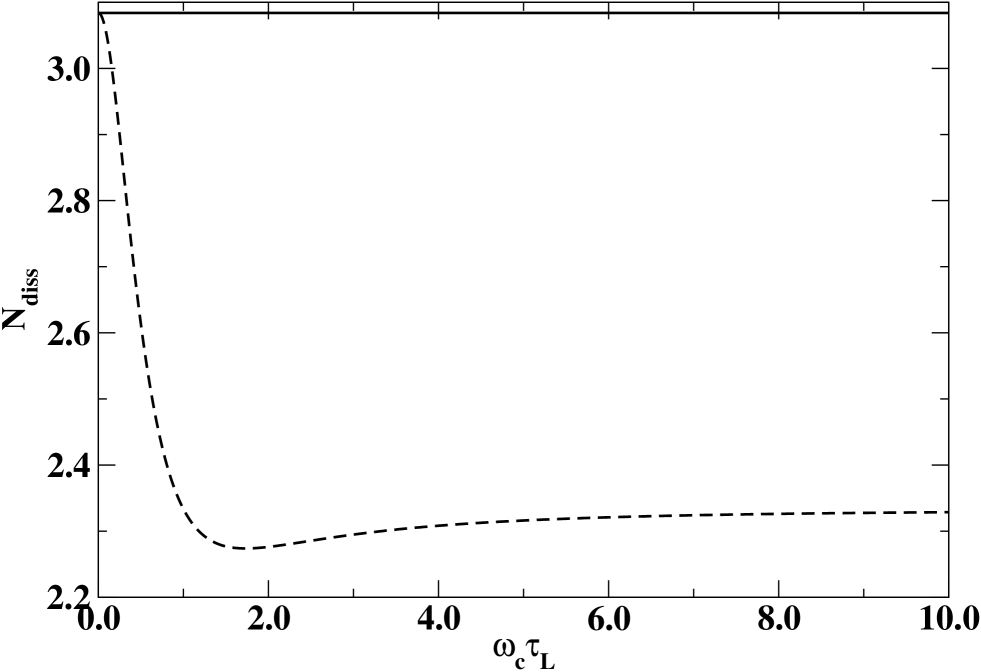
Figure 2: Variation of the negativity ${\cal N}_{\mathrm{diss}}$ with time in units of the bath high-frequency cut-off, $\omega_{c}\tau_{L}$ for a fixed squeezing parameter $|\zeta|=0.5$ and $p=1$ accounting for (dashed line) and not accounting for (solid line) the bath fluctuations. The other parameters are $\omega_{c}=2.62\times 10^{10}$ Hz, $\tau=4.325\times 10^{-12}$ s, and error probability $\delta=5\times 10^{-2}$.

V Conclusions

In conclusion, we have discussed in detail, how one can preserve entanglement in a class of continuous variable non-Gaussian states against decoherence caused by coupling to a bosonic bath. Specifically, we have considered transmission of an entangled state of two bosonic modes through an optical fiber and developed a hybrid approach combing decoherence-free subspaces and bang-bang control to sustain the entanglement. We described the non-Markovian interaction with the bosonic bath consisting of molecules in the fiber and provided a detailed estimate of the relevant parameters to implement our approach in a realistic fiber. It turns out that to achieve a loss figure of $<5\times 10^{-2}$ in a 1 km fiber, phase shifters should be placed about 1 mm apart. This appears to be a technologically feasible requirement. Hence we expect that the method proposed here will become a useful tool in the effort to transmit non-Gaussian entangled states over optical fibers.

References

- (1) V. Giovannetti, S. Guha, S. Lloyd, L. Maccone, J. H. Shapiro, and H. P. Yuen, Phys. Rev. Lett. 92, 027902 (2004).
- (2) S. D. Bartlett, B. C. Sanders, S. L. Braunstein, and K. Nemoto, Phys. Rev. Lett. 88, 097904 (2002); S. D. Bartlett and B. C. Sanders, Phys. Rev. Lett. 89, 207903 (2002).
- (3) J. Eisert, S. Scheel, and M. B. Plenio, Phys. Rev. Lett. 89, 137903 (2002).
- (4) G. S. Agarwal and A. Biswas, New J. Phys. 7, 211 (2005).
- (5) E. Shchukin and W. Vogel, Phys. Rev. Lett. 95, 230502 (2005).
- (6) M. Hillery and M. S. Zubairy, Phys. Rev. Lett. 96, 050503 (2006).
- (7) C. H. Bennett, G. Brassard, S. Popescu, B. Schumacher, J. A. Smolin, and W. K. Wootters, Phys. Rev. Lett. 76, 722 (1996); C. H. Bennett, D. P. DiVincenzo, J. A. Smolin, and W. K. Wootters, Phys. Rev. A 54, 3824 (1996).
- (8) D. Deutsch, A. Ekert, R. Jozsa, C. Macchiavello, S. Popescu, and A. Sanpera, Phys. Rev. Lett. 77, 2818 (1996).
- (9) H.-J. Briegel, W. Dür, J.I. Cirac, P. Zoller, Phys. Rev. Lett. 81, 5932 (1998); W. Dür, H.-J. Briegel, J. I. Cirac, and P. Zoller, Phys. Rev. A 59, 169 (1999).
- (10) L.-A. Wu, D. A. Lidar, and S. Schneider, Phys. Rev. A 70, 032322 (2004).
- (11) G. Compagno, A. Messina, H. Nakazato, A. Napoli, M. Unoki, and K. Yuasa, Phys. Rev. A 70, 052316 (2004).
- (12) L.-M Duan and G.-C. Guo, Phys. Rev. Lett. 79, 1953 (1997); P. Zanardi and M. Rasetti, Phys. Rev. Lett. 79, 3306 (1997); D. A. Lidar, I. L. Chuang, and K. B. Whaley, Phys. Rev. Lett. 81, 2594 (1998); D. A. Lidar and K. B. Whaley, Irreversible Quantum Dynamics, F. Benatti and R. Floreanini (Eds.), p. 83 (Springer Lecture Notes in Physics, 622, Berlin, 2003).
- (13) L. Viola and S. Lloyd, Phys. Rev. A 58, 2733 (1998); P. Zanardi, Phys. Lett. A 258, 77 (1999); L.-M Duan and G. C. Guo, Phys. Lett. A 261, 139 (1999); L. Viola, E. Knill, and S. Lloyd, Phys. Rev. Lett. 82, 2417 (1999); M. S. Byrd and D. A. Lidar, Quant. Info. Proc. 1, 19 (2002); P. Facchi, D.A. Lidar, and S. Pascazio, Phys. Rev. A 69, 032314 (2004).
- (14) L.-A. Wu and D. A. Lidar, Phys. Rev. A 70, 062310 (2004).
- (15) M. S. Byrd and D. A. Lidar, Phys. Rev. Lett. 89, 047901 (2002).
- (16) D. A. Lidar and L.-A. Wu, Phys. Rev. A 67, 032313 (2003).
- (17) G. S. Agarwal and K. Tara, Phys. Rev. A 43, 492 (1991).
- (18) G. S. Agarwal, R. R. Puri, and R. P. Singh, Phys. Rev. A 56, 4207 (1997).
- (19) G. S. Agarwal, Quant. Opt. 2, 1 (1990); G. M. D’Ariano, P. Kumar, C. Macchiavello, L. Maccone, and N. Sterpi, Phys. Rev. Lett. 83, 2490 (1999).
- (20) K. Watanabe and Y. Yamamoto, Phys. Rev. A 38, 3556 (1998).
- (21) A. Zavatta, S. Viciani, and M. Bellini, Science 306, 660 (2004).
- (22) R. García-Patrón, J. Fiurás̆ek, N. J. Cerf, J. Wenger, R. Tualle-Brouri, and P. Grangier, Phys. Rev. Lett. 93, 130409 (2004); R. García-Patrón, J. Fiurás̆ek, and N. J. Cerf, Phys. Rev. A 71, 022105 (2005).
- (23) A. Peres, Phys. Rev. Lett. 77, 1413 (1996); M. Horodecki, P. Horodecki, and R. Horodecki, Phys. Lett. A 223, 1 (1996).
- (24) G. Vidal and R. F. Werner, Phys. Rev. A 65, 032314 (2002).
- (25) C. Cohen-Tannoudji,, J. Dupont-Roc, and G. Grynberg, Atom-Photon Intercations: Basic Processes and Applications (Wiley, New York, 1998), p. 101.
- (26) M.W. Reinsch, J. Math. Phys. 41, 2434 (2000).
- (27) M.S. Byrd and D.A. Lidar, Phys. Rev. A 67, 012324 (2003).
- (28) G. P. Agarwal, Fiber-optic Communication Systems (Wiley, New York, 1992), Sec. 2.5 and Fig. 2.15.
- (29) M. O. Scully and M. S. Zubairy, Quantum Optics (Cambridge, Cambridge, 1997), Sec. 8.1.
- (30) G. W. Ford, J. T. Lewis, and R. F. O’Connell, Phys. Rev. Lett. 55, 2273 (1985); Phys. Rev. A 37, 4419 (1988).
- (31) J. J. Freeman and A. C. Anderson, Phys. Rev. B 34, 5684 (1986).
- (32) C. L. Reynolds, J. Non-Cryst. Solids 37, 125 (1980).