$M$-body Pure State Entanglement
Feng Pan,^a,b, and J. P. Draayer^{b a}Department of Physics, Liaoning Normal University, Dalian 116029, P. R. China^bDepartment of Physics and Astronomy, Louisiana State University, Baton Rouge, LA 70803-4001

Abstract: The simple entanglement of $N$-body $N$-particle pure states is extended to the more general $M$-body or $M$-body $N$-particle states where $N\neq M$. Some new features of the $M$-body $N$-particle pure states are discussed. An application of the measure to quantify quantum correlations in a Bose-Einstien condensate model is demonstrated.

Keywords: Many-body pure state, entanglement measure, quantum correlations. PACS numbers: 03.67.-a; 03.67.Mn; 03.65.Ud; 03.65.Bz

1 Introduction

Entanglement plays an important role in quantum information theory and quantum computation [1]-[3]. Entanglement normally considered is about $N$-body $N$-particle states. The most famous and widely studied of these are probably the Bell states [4] with $N=2$, and $N$-body $N$-particle GHZ [5] and W [6] states with $N\geq 3$. Often, however, that the number of particles $N$ is not equal to the number of kinds of particles $M$ in a quantum state. Such multipartite entangled states can be generated naturally in numerous many-body quantum systems, such as spin systems [7]-[9], one dimensional chains or lattices of various dimensions of Bose or Fermi many-body systems [10]-[12] including two-body $N$-particle entangled states generated in the Bose-Einstein condensate [13] with sufficiently large $N$, of which physical systems can be fabricated with modern technology. Specifically, entangled states can be realized by burning the system into a desired configuration and then cooling it down, which leads to the so-called ground state entanglement [14]. In order to classify different entangled states and study the entanglement of these types of states, it is necessary to extend the definition of entanglement to $M$-body $N$-particle pure states where $N\neq M$. Up till now, there have been at least four different approaches to the problem, namely, the entanglement of modes [15], the quantum correlations [16], the entanglement of particles [17], and entanglement witness [18]. The entanglement of modes proposed by Zanardi [15] is defined in terms of local entanglement in terms of local reduced density matrix in Fock representation. The quantum correlations for pure states introduced in [16] are determined by the so-called Slater rank of the state. The entanglement of particles provides an operational definition of entanglement between two parties who share an arbitrary pure state with a standard measure [17]. Finally, entanglement of witness is defined in [18] based on witness operators. Each of these approaches emphasizes one or several respects of the problem. There is still no consensus reached on which one is the most suitable.

As an extension of the entanglement measure for $N$-body $N$-particle pure states [19], in this paper, we propose an entanglement measure for $M$-body $N$-particle states for any $M$ and $N$, which can be regarded as an extension of the entanglement of modes proposed by Zanardi [15], but does not count in entanglement among local identical (indistinguishable) particles. In Sec. 2, we will propose the entanglement measure for $M$-body $N$-particle pure states for any $M$ and $N$. Some simple examples taken from quantum many-body systems will be analyzed with this measure in Sec. 3. Sec. 4 is a short discussion.

2 The entanglement measure for $M$-body $N$-particle pure states

For a system consisting of $M$ kinds of particles, any pure state $|\Psi\rangle$ can be expanded in terms of basis vectors $|n_{1},\sigma_{1};n_{2},\sigma_{2};\cdots;n_{M},\sigma_{M}\rangle$ in the tensor product space $V_{k_{1}}\otimes V_{k_{2}}\otimes\cdots\otimes V_{k_{M}}$ as

$$|\Psi\rangle=\sum_{n_{1}\sigma_{1}n_{2}\sigma_{2}\cdots n_{M}\sigma_{M}}C^{n_{1}n_{2}\cdots n_{M}}_{\sigma_{1}\sigma_{2}\cdots\sigma_{M}}|n_{1},\sigma_{1};n_{2},\sigma_{2};\cdots;n_{M},\sigma_{M}\rangle,$$

where $n_{i}$ ($1\leq i\leq M$) is the number of the $i$-th kind of particle, $\sigma_{i}=0,1,\cdots,k_{i}$  for $1\leq i\leq M$ denotes the internal degrees of freedom, and $C^{n_{1}n_{2}\cdots n_{M}}_{\sigma_{1}\sigma_{2}\cdots\sigma_{M}}$ is the normalized expansion coefficient. Then (1) will be called an $M$-body pure state. In addition, if the total number of particles $\hat{N}=\sum_{i=1}^{M}\hat{n}_{i}$ is a conserved quantity with

$$\hat{N}|\Psi\rangle=N|\Psi\rangle,$$

(1) will be called an $M$-body $N$-particle pure state, which will be denoted as $|\Psi(M,N)\rangle$ in the following. According to the above definition, Bell states are two-body two-particle states, GHZ and W states are $N$-body $N$-particle states with $N\geq 3$. The corresponding density matrix of (1) is

$${\rho}_{\Psi}=|\Psi\rangle\langle\Psi|.$$

Let $a_{i\sigma}^{\dagger}$ ($a_{i\sigma}$) be local particle creation (annihilation) operators that satisfy

$$[a_{i\sigma},a_{j\sigma^{\prime}}^{\dagger}]_{\pm}\equiv a_{i\sigma}a_{j\sigma^{\prime}}^{\dagger}\pm a_{j\sigma^{\prime}}^{\dagger}a_{i\sigma}=\delta_{ij}\delta_{\sigma\sigma^{\prime}},$$

$$[a_{i\sigma},a_{j\sigma^{\prime}}]_{\pm}=[a^{\dagger}_{i\sigma},a_{j\sigma^{\prime}}^{\dagger}]_{\pm}=0,$$

for fermions or bosons. The wavefunction $|\Psi(M,N)\rangle$ can be expressed as

$$|\Psi(M,N)\rangle=\sum_{n_{1}\sigma_{1}\cdots n_{M}\sigma_{M}}C_{n_{1}\sigma_{1}\cdots n_{M}\sigma_{M}}(a_{1}^{\dagger})_{\sigma_{1}}^{n_{1}}(a_{2}^{\dagger})_{\sigma_{2}}^{n_{2}}\cdots(a_{M}^{\dagger})_{\sigma_{M}}^{n_{M}}|0\rangle,$$

where $|0\rangle$ is the vacuum state and $(a_{i}^{\dagger})_{\sigma_{i}}^{n_{i}}\equiv\sum_{\sigma^{i}_{1}\sigma^{i}_{2}\cdots\sigma^{i}_{n_{i}}}\beta^{\sigma_{i}}_{\sigma^{i}_{1}\sigma^{i}_{2}\cdots\sigma^{i}_{n_{i}}}a_{i\sigma^{i}_{1}}^{\dagger}a_{i\sigma^{i}_{2}}^{\dagger}\cdots a_{i\sigma^{i}_{n_{i}}}^{\dagger}$, in which $\beta^{\sigma_{i}}_{\sigma^{i}_{1}\sigma^{i}_{2}\cdots\sigma^{i}_{n_{i}}}$ is the expansion coefficient.

In (1) and (6), $\{|n_{i}\sigma_{i}\rangle\}$ is recognized as a set of the local basis vectors for the $i$-th kind of particles, which can be used, for example, to describe a set of local states on the $i$-th site of a lattice in many lattice models. In such cases, only entanglement among particles on different sites is of interest, which can also be used to signify quantum correlations in a model system. Therefore, entanglement among particles on the same site will not be considered. Similar problems were also considered in many works. For example, hierarchic classification for arbitrary multi-qubit mixed states based on the separability properties of certain partitions was considered by Dür and Cirac in [20].

Under the replacement $a_{i\sigma^{i}_{j}}^{\dagger}\rightarrow X_{i\sigma^{i}_{j}}$, where $X_{i\sigma^{i}_{j}}$ is simply a symbol, the operator form in front of the vacuum state on the right-hand-side of (6) becomes a homogeneous polynomial of degree $N$ in terms of the $\{{\bf X}_{i}\}$,

$$F_{C}({\bf X}_{1},\cdots,{\bf X}_{M})=\sum_{\sigma_{1}\cdots\sigma_{N}}C_{\sigma_{1}\cdots\sigma_{N}}(X_{1})^{n_{1}}_{\sigma_{1}}\cdots(X_{M})^{n_{M}}_{\sigma_{M}}.$$

It should be understood that ${\bf X}_{i}$ is a multi-value symbol with ${\bf X}_{i}=X_{i\sigma^{i}_{j}}$ for any $\sigma^{i}_{j}$. An alternative definition of entangled states with respect to the local bases can be stated as follows: The state $|\Psi(M,N)\rangle$ is an $M$-body $N$-partite entangled state if the corresponding polynomial $F_{C}({\bf X}_{1},\cdots,{\bf X}_{M})$ on complex field ${\bf\cal C}$ cannot be factorized into the following form

$$F_{C}({\bf X}_{1},\cdots,{\bf X}_{M})=F_{A}({\bf X}_{i_{1}},\cdots,{\bf X}_{i_{l}})F_{B}({\bf X}_{i_{l+1}},\cdots,{\bf X}_{i_{M}})$$

for $1\leq l\leq M-1$, where $\{i_{1}\neq i_{2}\neq\cdots\neq i_{M}\}$ can be in any ordering of $\{1,2,\cdots,M\}$. Otherwise the state $|\Psi(M,N)\rangle$ is not an $M$-body $N$-particle entangled state with respect to the $M$ sets of local bases. The state $|\Psi(M,N)\rangle$ given in (6) is disentangled (separable) if the polynomial $F_{C}$ can be factorized into a product of polynomials of ${\bf X}_{i}$ as $\prod_{i=1}^{M}F_{A_{i}}({\bf X}_{i})$. In other cases, the state is partially entangled.

As is shown in [19], a criterion for distinguishing whether a homogeneous polynomial is factorizable can be established by using the von Neumann entropy of the reduced local density matrices. As an extension of the entanglement measure [19] for $N$-body $N$-partical qubit system, we define entanglement measure for the $M$-body pure state (1) as

$$\eta^{(M)}=\left\{\matrix{{1\over{M}}\sum^{M}_{i}S_{(i)},~{}~{}~{}{\rm if}~{}~{}S_{i}\neq 0~{}~{}\forall~{}~{}i,\cr\cr~{}~{}~{}0~{}~{}~{}~{}~{}~{}~{}~{}~{}~{}~{}~{}~{}{\rm otherwise,}\cr}\right.$$

where $M$ is the number of different kinds of particles involved in (1),

$$S_{(i)}=-{\rm Tr}[\rho_{(i)}\log_{p_{i}}(\rho_{(i)})]$$

is the extended local reduced von Neumann entropy expressed in terms of local reduced density matrix $\rho_{(i)}$ for the $i$-th kind of particles only obtained by taking the partial trace over the subsystem, and $p_{i}$ is the total number of the Fock states of the $i$-th kind of particles in the system. We use the logarithm to the base $p_{i}$ instead of base $2$ used in qubit system [19] to ensure that the maximal measure is normalized to $1$. Hence, the maximal value of the measure is $1$ regardless how many particles and how many kinds of particles are involved in the system. While the measure is zero when a pure state is not a genuine $M$-body entangled state.

Similar to the $N$-body $N$-particle case [19], the measure (9) quantifies genuine $M$-body entanglement. The measure is zero if $S_{i}=0$ for any $1\leq i\leq M$, in which the corresponding state is not a genuine $M$-body entangled one. In contrast to the measure defined in terms of local von Neumann entropy [16], which provides information of local entanglement only, the measure (9) provides information about overall quantum correlations among $M$ kinds of particles in a quantum many-body system.

In the pure state (6), the local particle number is not a conserved quantity in general. In such a case, the local reduced density matrix $\rho_{(i)}$ is built in the local Fock space spanned by $\{|n_{i}\sigma_{i}\rangle\}$ ($0\leq n_{i}\leq p_{i}$) with the following block-diagonal form:

$$\rho_{(i)}=\left(\matrix{(n_{i}=0)\cr&(n_{i}=1)\cr&&(n_{i}=2)\cr&&~{}~{}~{}~{}~{}~{}~{}~{}\ddots\cr&&&(n_{i}=p_{i})\cr}\right),$$

where each sub-matrix $(n_{i}=q)$ is spanned by the $q$-particle Fock states with the internal degrees of freedoms $0\leq\sigma_{i}\leq k_{i}$. Therefore, the extended reduced von Neumann entropy $S_{(i)}$ is not only invariant under the Local Unitary (LU) transformations for each block in (11) with respect to internal degrees of freedoms $\{\sigma_{i}\}$ for fixed $n_{i}$, but also invariant under unitary transformations for the subspace spanned by the entire Fock states with the local particle numbers $0\leq n_{i}\leq p_{i}$. Hence, the measure (9) is also invariant under both the Local Unitary (LU) transformations with respect to internal degrees of freedoms and unitary transformations for the subspace spanned by the entire Fock states. In addition, the measure does not count in entanglement among local identical particles with the same label $i$ and different internal degrees of freedom because the local basis vectors are recognized to be $\{|n_{i}\sigma_{i}\rangle\}$.

In the $M=N$ qubit cases discussed in [19], the LU invariance is equivalent to the invariance under Local Operations assisted by Classical Communications (LOCCs). In such case the measure (9) is both LU and LOCC invariant [21]. In $N\neq M$ cases, however, LOCCs may be useless in any quantum information processing protocol. For example, LOCCs will not only keep the entanglement the same, but also be irrelevant to any quantum information processing processes for $M\neq N$. In addition, though (9) is invariant under local unitary transformations with respect to different number of particles, such transformations will result in local state mixing among different number of particles, which obviously violates the super-selection rule, and thus is impossible [22, 23, 24]. However, the measure (9) is indeed useful in quantifying the $M$-body $N$-particle entanglement, of which some examples will be shown in the next section.

3 Some simple examples

Using the above definition, one can easily write out many non-trivial states with $M\neq N$ which are quite different from those with $M=N$. For simplicity, let us assume that there are $M$ kinds of spinless fermions or bosons. Then, the simplest case is a $M$-body one-particle state with

$$|\Psi(M,1)\rangle=C_{1}|\overbrace{10\cdots 0}^{M}\rangle+C_{2}|\overbrace{010\cdots 0}^{M}\rangle+\cdots+C_{M}|\overbrace{0\cdots 01}^{M}\rangle,$$

where $|{0\cdots 010\cdots 0}\rangle$ with $1$ in the $i$-th position denotes one-particle state for the $i$-th kind of particle and vacuum state of the remaining particles, and $C_{i}$ ($i=1,2,\cdots,M$) are normalized non-zero expansion coefficients. These types of states emerge naturally from many models, such the Bose- and Fermi-Hubbard models.

In $N$-body $N$-particle cases, generally a state is entangled with respect to its intrinsic degrees of freedom, such as the third component of spin of photons or atoms. In such cases, the measure (9) is invariant under LOCCs or LUs. In $N\neq M$ cases, however, LOCCs may be useless in any quantum information processing protocol. In order to make this point clear, for example, let us replace spinless fermions or bosons in (12) by those with internal degrees of freedom $\sigma_{i}=1,2,\cdots,\mu_{i}$ for $i=1,2,\cdots,M$. Then, (12) becomes

$$|\Psi(M,1)(\sigma_{1}\sigma_{2}\cdots\sigma_{M})\rangle=C_{1}|\overbrace{1_{\sigma_{1}}0\cdots 0}^{M}\rangle+C_{2}|\overbrace{01_{\sigma_{2}}0\cdots 0}^{M}\rangle+\cdots+C_{M}|\overbrace{0\cdots 01_{\sigma_{M}}}^{M}\rangle.$$

$\mu_{i}$ should be all the same for any $i$ if these are identical particles, otherwise they are not identical. In this case, any LOCC between $i$-th and $j$-th parties is equivalent to a corresponding LU transformation with respect to the internal degrees of freedom labeled by $\sigma_{i}$ or $\sigma_{j}$. After any such LU transformation, say at $i$-th party, the vacuum state of the $i$-th particle for any $i$ remains invariant, while local one-particle state still remains to be one-particle state with a linear combination of different internal labels. The $j$-th party can not get any information after local operation at $i$-th party assisted by classical communication between them and then measuring the resultant $j$-th local state because the $j$-th state remains to be the same after any local operation at $i$-th party. Therefore, LOCCs will not only keep the entanglement the same for the state shown in (12), but also be irrelevant to any quantum information processing processes used in $M=N$ cases even if those $M$ Fock states have additional intrinsic degrees of freedom as shown in (13). Actually, $N\neq M$ entangled states, such as that shown in (13), are entangled with respect to local particle numbers in $M$ different local Fock states and not with respect to local intrinsic degrees of freedom. For a state, such as that shown in (13), effective local operations similar to those used in $M=N$ cases are local particle number non-conserved unitary operations, namely local projective operations, $a|0\rangle+b|1\rangle$, where $|0\rangle$ stands for vacuum state, $|1\rangle$ stands for one particle state, and $a,~{}b\in\bf C$ with $|a|^{2}+|b|^{2}=1$. As for entanglement in spin degrees of freedom, in which any local operation may violate conservation of spin in the third component, any local particle number non-conserved unitary operation violates both local and total particle number conservation. Such operations obviously violate the super-selection rule, and thus are impossible to be implemented. While the entanglement measure (9) is invariant under any such local particle number non-conserved operation.

Although local particle number non-conserved operations are physically impossible, measure (9) can be used to quantify entanglement of any $M$-body entangled state. For example, according to (9), the entanglement measure for (12) is

$$\eta^{(M,N=1)}=-{1\over{M}}\sum^{M}_{i=1}\left(|C_{i}|^{2}\log_{2}(|C_{i}|^{2})+(1-|C_{i}|^{2})\log_{2}(1-|C_{i}|^{2})\right).$$

It can be verified by conditional maximization that (12) reaches its maximal value when $|C_{i}|=1/\sqrt{M}$ with $M\geq 2$. Clearly, in the cases with maximal measure

$$\eta^{(M,N=1)}_{\max}=\log_{2}(M)-{M-1\over{M}}\log_{2}(M-1)~{}~{}{\rm for}~{}~{}~{}M\geq 2.$$

It is similar to the Bell states with $\eta^{(2,1)}_{\max}=1$ when $M=2$, and is equivalent to the W states with $\eta^{(3,1)}_{\max}=0.918296$ when $M=3$, which is the same value as that of a W state for a qubit system calculated in [25].

Though there is controversy about whether such states as that shown in (12) are entangled or not [26, 27], it was clearly demonstrated in [28] that such state is indeed a single-particle entangled state, which was also used in a two-party protocol for quantum gambling [29], and is proved to be useful in the so-called data hiding protocols [24]. The measure (9) is in agreement with those observations.

Another example of our application of the measure (9) is to study quantum phase transition in a Bose-Einstien condensate model with $n$ bosons in a two-dimensional harmonic trap interacting via a fairly universal contact interaction [30, 31, 32], of which the Hamiltonian can be written as

$$H=\sum^{\infty}_{j=0}\omega ja^{\dagger}_{j}a_{j}+g\sum_{i,j,k,l}\delta_{i+j,k+l}V_{i,j;k,l}a^{\dagger}_{i}a^{\dagger}_{j}a_{k}a_{l},$$

where $a^{\dagger}_{i}$ ($a_{i}$) is creation (annihilation) operator of the $i$-th boson, and $V_{ij;kl}=(k+l)!/(i!j!k!l!4^{k+l})^{1\over{2}}$. In this model, the total number of bosons $\hat{n}$ and the angular momentum $\hat{L}$ with

$$\hat{n}=\sum_{i=0}^{\infty}a_{i}^{\dagger}a_{i},~{}~{}\hat{L}=\sum_{j=0}^{\infty}ja_{j}^{\dagger}a_{j}$$

are two conserved quantities. Therefore, for given $n$ and $L$, eigenstates of (16) can be written as

$$|n,L;\tau\rangle=\sum_{n_{2}n_{3}\cdots n_{L}}c^{\tau}_{n_{2}n_{3}\cdots n_{L}}{a_{0}^{\dagger}}^{n-L+\sum_{\mu=2}^{L}(\mu-1)n_{\mu}}\times$$

$${a_{1}^{\dagger}}^{L-\sum_{\mu=2}^{L}\mu n_{\mu}}a_{2}^{\dagger n_{2}}a_{3}^{\dagger n_{3}}\cdots a_{L}^{\dagger n_{L}}|0\rangle,$$

where $c^{\tau}_{n_{2}n_{3}\cdots n_{L}}$ are expansion coefficients, and $\tau$ is an additional quantum number needed in distinguish different eigenstates with the same $n$ and $L$.

To explore transitional patterns in the system, we calculate the entanglement according to (9) along the yrast line up to $L=6$, in which the local reduced density matrices $\rho_{(i)}$ for the $i$-th kind of bosons are obtained by taking the partial trace over the subsystem. Fig. 1 shows the entanglement measure (9) of the system as a function of the total number of bosons $n$ along the yrast line with $L=2,~{}3,\cdots,~{}6$. Generally speaking, the maximal value of the measure decreases with $L$; and the measure for any $L$ decreases with increasing of $n$ due to the $s$-boson dominance in the yrast states when $n$ is sufficiently large. It is obvious that there is always a peak in the measure at or near $n=L+1$ when $L\geq 4$. The peak in the entanglement measure signify that there is a quantum phase transition occurring near $n=L+1$, in which the total number of bosons $n$ serves as the control parameter.

In order to show that the peak point in the entanglement measure shown in Fig. 1 indeed is a critical point of the system, we study yrast state occupation probabilities $\xi_{l}(n)$ for bosons with different angular momentum $l$ as a function of $n$ according to

$$\phi_{l}(n)=\langle a^{\dagger}_{l}a_{l}\rangle/n.$$

The results for $L=2$, $3$, $4$, $5$ cases are shown in Fig. 2, which shows that the values of the occupation probabilities for bosons with different angular momentum vary drastically with increasing of the total number of bosons, especially for $s$- and $p$-bosons. When $n=L$, the $l$-boson, especially the $p$-boson components contribute significantly to the yrast states. There are cross points for yrast state occupation probabilities $\phi_{l}(n)$ with different $l$, which are indeed all near $n=L+1$ point. The $L=4$ and $L=5$ cases shown in Fig. 2 are consistent to the critical points at the entanglement measures shown in Fig. 1 though it is not shown by the entanglement measures in Fig. 1 for $L=2$ and $3$ cases. The results show that there are two different phases. One is the $p$-boson dominant phase, while another is the $s$-boson dominant phase, which are controlled by the total number of bosons in the system. Therefore, the peak in the entanglement measure indeed signifies that there is a quantum phase transition occurring near $n=L+1$, in which the total number of bosons $n$ serves as the control parameter. The result also shows that the measure (9) is indeed suitable to benchmark the quantum correlations among bosons with different angular momenta.

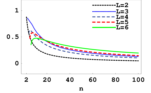
Figure 1: The entanglement measure $\eta^{(L+1)}$ as functions of the total number of bosons $n$ along the yrast line up to $L=6$.

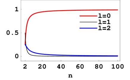
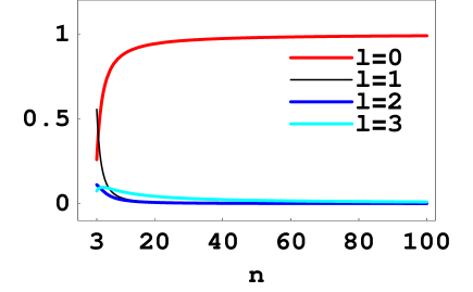
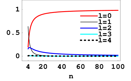
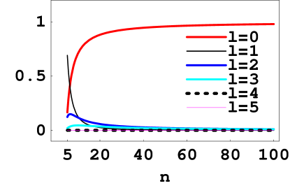
Figure 2: Occupation probabilities $\phi_{l}(n)$ with $l=0,1,\cdots,L$ as functions of $n$ along the yrast line up to $L=5$, where the upper left panel is for $L=2$, the upper right one is for $L=3$, the lower left one is for $L=4$, and the lower right one is for $L=5$, respectively.

4 Discussion

In conclusion, entanglement of $M$-body and $M$-body $N$-particle pure states is defined. The simple entanglement measure formerly defined for $M=N$ multipartite pure states is extended to the general cases with any $M$ and $N$. The feature of the measure is that it only count in entanglement among non-identical particles. For example, the measure does not count in entanglement among particles with different internal degrees of freedom on the same site in lattice models, and so on, which seems to be a natural way to define entanglement in quantum many-body problems.

Though the measure is defined for pure states, it can easily be extended to the measure for mixed states $\rho$ by the convex roof construction with [33]

$$\eta(\rho)=\min_{\Phi}\sum_{i}q_{i}\eta(|\Psi_{i}\rangle\langle\Psi_{i}|),$$

where $\Phi$ is the set of ensembles realizing the density matrix $\rho$ with $\Phi=(\{q_{i},|\Psi_{i}\rangle\}~{}~{}|~{}\rho=\sum_{i}q_{i}|\Psi_{i}\rangle\langle\Psi_{i}|$,
$\sum_{i}q_{i}=1)$.

An example of application of the $M$-body $n$-particle pure state entanglement measure to the Bose-Einstien condensate model with $n$ bosons in a two-dimensional harmonic trap interacting via a fairly universal contact interaction is provided, which shows that the measure is effective to quantify entanglement or quantum correlations among different kinds of particles in the system. Therefore, the proposed entanglement measure is useful not only in quantifying entanglement, but also in studying quantum phase transitions in quantum many-body systems with sufficiently large number of particles.

Support from the U.S. National Science Foundation (0140300; 0500291), the Southeastern Universitites Research Association, the Natural Science Foundation of China (10175031; 10575047), and the LSU–LNNU joint research program (C192135) is acknowledged.

References

- [1] M. A. Nielsen and I. L. Chuang, Quantum Information and Computation, (Cambridge Univ. Press, 2000).
- [2] C. H. Bennett and D. P. DiVincenzo, Nature (London) 404 (2000) 247.
- [3] B. M. Terhal, M. M. Wolf, and A. C. Doherty, Phys. Today 56 (2003) 46.
- [4] J. S. Bell, Physics (N.Y.) 1 (1964) 195.
- [5] D. M. Greenberger, M. A. Horne, A. Zeilinger, in M. Kafatos (Ed.), Bell’s Theorem, Quantum Theory, and Conceptions of the Universe (Kluwer, Dordrecht, 1989) p. 69.
- [6] W. Dür, G. Vidal, J. I. Cirac, Phys. Rev. A 62 (2000) 062314.
- [7] A. Søensen and K. Mømer, Phys. Rev. Lett. 83 (1999) 2274.
- [8] K. M. O’Connor and W. K. Wootters, Phys. Rev. A 63 (2001) 052302.
- [9] L.-M. Duan, E. Demler, and M. D. Lukin, Phys. Rev. Lett. 91 (2003) 090402.
- [10] M. Greiner, O. Mandel, T. Esslinger, T. W. Hänsch, and I. Bloch, Nature (London) 415 (2002) 39.
- [11] D. Jaksch and P. Zoller, Ann. Phys. 315 (2005) 52.
- [12] A. Griessner, A. J. Daley, D. Jaksch, and P. Zoller, Phys. Rev. A 72 (2005) 032332.
- [13] Feng Pan and J. P. Draayer, Phys. Lett. A 339 (2005) 403.
- [14] A. Hutton and S. Bose, Phys. Rev. A 69 (2004) 042312
- [15] P. Zanardi, Phys. Rev. A 65 (2002) 042101.
- [16] J. Schliemann, J. I. Cirac, M. Kus, M. Lewenstein, and D. Loss, Phys. Rev. A 64 (2001) 022303.
- [17] H. M. Wiseman and J. A. Vaccaro, Phys. Rev. Lett. 91 (2003) 097902.
- [18] F. G. S. L. Brandão, Phys. Rev. A 72 (2005) 022310.
- [19] Feng Pan, Dan Liu, Guoying Lu, J. P. Draayer, Int. J. Theor. Phys. 43 (2004) 1241.
- [20] Dür and Cirac, Phys. Rev. A 61 (2000) 042314.
- [21] R. Srikanth, arXiv: quant-ph/0601062 v1.
- [22] N. Schuch, F. Verstraete, and J. I. Cirac, Phys. Rev. Lett. 92 (2004) 087904.
- [23] S. D. Bartlett and H. M. Wiseman, Phys. Rev. Lett. 91 (2003) 097903.
- [24] F. Verstraete and J. I. Cirac, Phys. Rev. Lett. 91 (2003) 010404.
- [25] Feng Pan, Dan Liu, Guoying Lu, J. P. Draayer, Phys. Lett. A 336 (2005) 384.
- [26] C. C. Gerry, Phys. Rev. A 53 (1996) 4583.
- [27] Y. Aharonov and L. Vaidman, Phys. Rev. A 61 (2000) 052108.
- [28] S. J. van Enk, Phys. Rev. A 72 (2005) 064306.
- [29] Lior Goldenberg, Lev Vaidman, and Stephen Wiesner, Phys. Rev. Lett. 82 (1999) 3356.
- [30] B. Mottelson, Phys. Rev. Lett. 83 (1999) 2695.
- [31] N. K. Wilkin, J. M. Gunn, and R. A. Smith, Phys. Rev. Lett. 80 (1998) 2265.
- [32] G. F. Bertsch and T. Pappenbrock, Phys. Rev. Lett. 83 (1999) 5412.
- [33] P. J. Love, A. Yu Smirnov, A. M. van den Brink, M. H. S. Amin, M. Grajcar, E. Il ichev, A. Izmalkov, and A. M. Zagoskin, arXiv: quant-ph/0602143 v1.