Statistical properties of the truncated state with random coefficients

Abstract

In this paper we introduce the truncated state with random coefficients (TSRC). As the coefficients of the TSRC have in principle no algorithm to produce them, our question is concerned about to what type of properties will characterize the TSRC. A general method to engineer TSRC in the running-wave domain is employed, which includes the errors due to the nonidealities of detectors and photocounts.

I Introduction

The generation of new states of the light field turned out to be an important topic in quantum optics in the last years, such as quantum teleportation bennett93 , quantum computation Kane98 , quantum communication Pellizzari97 , quantum cryptography Gisin02 , quantum lithography Bjork01 , decoherence of states Zurek91 , etc. The usefulness and relevance of quantum states, to give a few examples, cover the study of i) quantum decoherence effects in mesoscopic fields harochegato ; ii) entangled states and quantum correlations brune ; interference in the phase space bennett2 ; collapses and revivals of the atomic inversion narozhny ; engineering of (quantum states) reservoir zoller ; etc. Also, it is worth mentioning the importance of the statistical properties of one state to determine some relevant properties of another barnett as well as using specific quantum states as input to engineer a desired state serra .

Here we introduce a truncated state having random coefficients (TSRC). This state is characterized by a constant phase relation between the relative Fock states, but with coefficients describing probability amplitudes obtained through some random number generator. Features of this state are studied by analyzing several of its statistical properties. We believe the TSRC can be a useful tool to test sequence of numbers whose generation is unknown from the observer. Indeed, preliminary results have corroborated this expectation wesley .

This paper is organized as follows: in Section II we introduce the TSRC and Section III we analyze the behaviour of some statistical properties of the TSRC when the Hilbert space is increased. In Section IV we show how to engineer TSRC in the running-wave domain, and Section V is devoted to the study of losses due to nonidealities of the detectors in the whole process of engineering. Finally, in Section VI we present our conclusions.

II Truncated states with random coefficients (TSRC)

We define the TSRC as

$$\left|TSRC\right\rangle=\mathcal{N}\sum\limits_{n=0}^{N}r_{n}e^{in\theta}\left|n\right\rangle$$ (1)

where $\mathcal{N}$ is a normalization constant and $C_{n}=r_{n}e^{in\theta}$ is a random complex coefficient (polar form), given by some random number generator (RNG). It is worthwhile to note that TSRC differs from (mixed) thermal states (MTS) and Pure States Having Thermal Photon Distribution (PSTD)Marhic , since these states have an algorithm for the coefficients $C_{n}{\prime}s$. In addition, although TSRC is a pure state, its statistical properties are very different from the PSTD: for example, the TSRC does not exhibit squeezing for $N\gtrsim 12$, as shown in the next section.

III Statistical properties of TSRC

III.1 Photon Number Distribution

Since the expansion of TSRC is known in the number state $\left|n\right\rangle$, we have

$$P_{n}=\mathcal{N}^{2}\left|C_{n}\right|^{2}.$$ (2)

Fig. $1-3$ show the plots of the photon-number distribution, $P_{n}$ versus $n$, for TSRC. Although the generation of  the TSRC be virtually impossible for Hilbert space dimensions $10^{4}$, due to nonidealities of beam splitters and detectors causing decoherence effects as well as due to low success probability (see section IV), it can be useful to study the behavior of TSRC for large $N$, specially when we are interested in investigate the properties of sequence of numbers wesley . Fig$-3$, which is a expanded view of the Fig. $2$, shows the same behavior of that of the Fig.$1$. As expected, when $N$ is large enough (Fig. 2 ), the difference from one peak to another becomes negligible. For small values of $n$, running the RNG several times will give different sets of numbers with different ${P_{n}}^{\prime}s$. Therefore, it is important to keep in mind that our proposal to generate TSRC is based on a particular set of numbers obtained by a single run of the RNG. Thus, these numbers, having no algorithm producing them, a question emerging is: what type of properties will characterize a state having a random probability amplitude? These properties will be investigated in the next subsections.

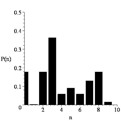
Figure 1: The photon number distribution $P_{n}$ of TSRC versus n for the dimension of Hilbert space $N=10$. This figure was obtained by a single run of the RNG.

Figure 2: The photon number distribution $P_{n}$ of TSRC versus $n$. As expected, when $N$ is large the difference from one peak to another becomes negligible. The dimension of Hilbert space here is $N=10000$. This figure was obtained by a single run of the RNG.

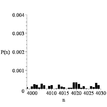
Figure 3: Expanded view of the photon number distribution $P_{n}$ of  the TSRC versus $n$ in the Fig.$2$. This figure was obtained by a single run of the RNG.

III.2 Average number and variance

The average number $\left\langle\hat{n}\right\rangle$ as well as the variance in TSRC is obtained directly from

$$\left\langle\hat{n}\right\rangle=\sum_{n=0}^{N}P(n)n\text{,}$$ (3)

and

$$\left\langle\Delta\hat{n}\right\rangle=\sqrt{\left\langle\hat{n}^{2}\right\rangle-\left\langle\hat{n}\right\rangle^{2}}\text{.}$$ (4)

Fig. $4$, $5$ show the plots of $\left\langle\hat{n}\right\rangle$ and $\left\langle\Delta\hat{n}\right\rangle$ as a function of the Hilbert space dimension $N$. Note from Fig.$3$ that $\left\langle\hat{n}\right\rangle$ increases irregularly with $N$ when a single realization is considered, but tends to increase linearly with $N$ when several realizations are considered. As can be seen from Fig.$5$, the increasing of $\left\langle\Delta\hat{n}\right\rangle$ with $N$ is irregular, irrespective of the number of realizations.

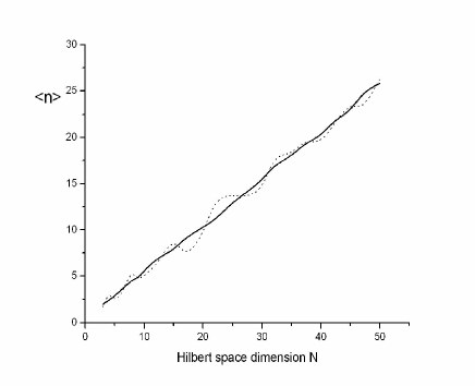
Figure 4: The average number $<n>$ versus the dimension $N$ of the Hilbert space. Solid line was obtained from 30 realizations of the RNG. Dots refer to a single one.

Figure 5: The variance $\langle\Delta n\rangle$ versus the dimension $N$ of the Hilbert space.

III.3 Mandel parameter and second order correlation function

Mandel Q parameter is defined as

$$Q=\frac{\left(\Delta\hat{n}^{2}-\left\langle\hat{n}\right\rangle\right)}{\left\langle\hat{n}\right\rangle}\text{,}$$ (5)

while the second order correlation function $g^{\left(2\right)}(0)$ is

$$g^{\left(2\right)}(0)=\frac{\left(\left\langle\hat{n}^{2}\right\rangle-\left\langle\hat{n}\right\rangle\right)}{\left\langle\hat{n}\right\rangle^{2}}\text{,}$$ (6)

and for $Q<0$ ($Q>0$) the state is said to be sub-poissonian (super-poissonian). Also, the $Q$ parameter and the second order correlation function $g^{\left(2\right)}$ are related by walls

$$Q=\left[g^{\left(2\right)}(0)-1\right]\left\langle\hat{n}\right\rangle\text{.}$$ (7)

It is well known that if $g^{\left(2\right)}(0)<1$ then the Glauber-Sudarshan P-function assumes negative values, thus differing from usual probability distribution function. Beside that, by Eq. (7) is readily seen that $g^{\left(2\right)}(0)<1$ implies $Q<0$. As for a coherent state $Q=0$, a state is said to be a “classical” one if $Q>0$.

Fig. $6$ and $7$ show the plots of the $Q$ parameter and the correlation function $g^{\left(2\right)}(0)$ versus $N$. It is interesting to note that the TSRC is predominantly super-poissonian ($Q>0$ and $g^{\left(2\right)}(0\dot{)}>1$) , then being a “classical” state in this aspect, for $N\gtrsim 12$. Nevertheless, for small values of  $N$ ($N<12$), the $Q$ parameter presents significant occurrence of values less than $0$, showing sub-poissonian statistics and thus being associated with a “quantum state”. However, when $N$ becomes larger than $12$, TSRC becomes super-poissonian. Also, note that for a single realization of the RNG these both functions present an oscillatory behavior, while, for several realizations, Fig.$6$ (solid line) shows an interesting linear dependence between $Q$ and $N$. This will be further investigated in the following subsection. On the other hand, Fig.$7$ indicates an asymptotic behavior of  $g^{\left(2\right)}(0\dot{)}$ when $N$ is increased. For $N=10^{4}$, we find $g^{\left(2\right)}(0\dot{)}=1.332585322$.

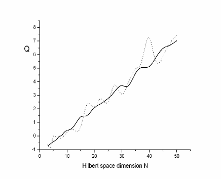
Figure 6: The $Q$ parameter versus $N$. For $N\gtrsim 12$, $Q>0$ and there is a linear dependence between $Q$ and $N$. Solid line was obtained from 30 realizations of the RNG. Dots refer to a single one.

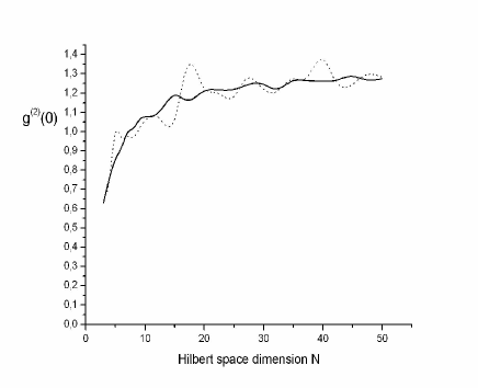
Figure 7: The $g^{(2)}(0)$ correlation function versus $N$. Solid line was obtained from 30 realizations of the RNG. Dots refer to a single one.

III.4 Quadrature and variance

Quadrature operators are defined as

$$X_{1} = \frac{1}{2}\left(a+a^{\dagger}\right);$$ (8)

$$X_{2} = \frac{1}{2i}\left(a-a^{\dagger}\right),$$ (9)

where $a$ ($a^{\dagger}$)  is the annihilation (creation) operator in Fock space. Quantum effects arise when the variance of one of the two quadrature attains a value $\Delta X_{i}<0.5$, $i=1,2$. Fig. $8$ and $9$ show the plots of quadrature variance $\Delta X_{i}=\sqrt{\left\langle X_{i}^{2}\right\rangle-\left\langle X_{i}\right\rangle^{2}}$ versus $N$. Note the same oscillatory behavior when a single realization of RNG is considered. For small $N$ ($N<12$), TSRC exhibits squeezing with a significant frequency (running RNG several times). On the other hand, when $N$ increases, squeezing becomes a rare event, and can be set a null event for $N\gtrsim 12$, coinciding with the departure from sub-poissonian statistic discussed above.

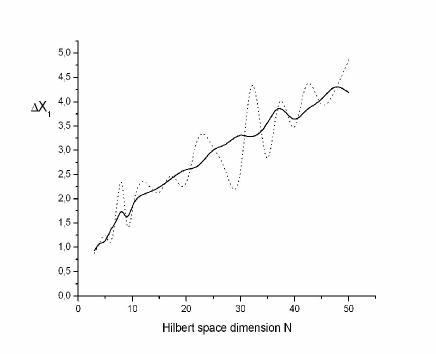
Figure 8: The $\Delta X_{1}$ quadrature variance versus the dimension $N$ of the Hilbert space. For $N\gtrsim 12$, squeezing can be considered a null event. Solid line was obtained from 30 realizations of the RNG. Dots refer to a single one.

Figure 9: The $\Delta X_{2}$ quadrature variance versus the dimension $N$ of the Hilbert space. For $N\gtrsim 12$, squeezing can be considered a null event. Solid line was obtained from 30 realizations of the RNG. Dots refer to a single one.

III.5 Entropy

Fig. $10$ shows the plots of Shannon entropy $S=\sum\limits_{n=0}^{N-1}P_{n}\ln P_{n}$ versus $N$. It shows a steady increasing of  $S$. In fact, increasing $N$ arbitrarily, we have found no bound for $S$, thus indicating no maximum for Shannon entropy.

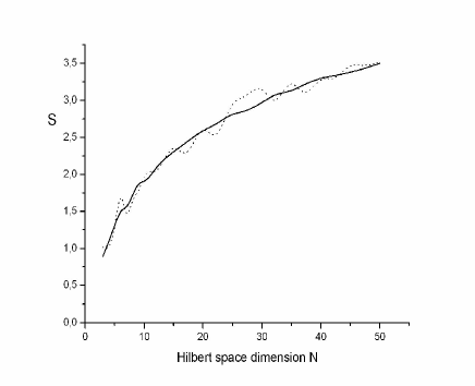
Figure 10: The $S$ Shannon entropy versus the dimension $N$ of the Hilbert space. Solid line was obtained from 30 realizations of the RNG. Dots refer to a single one.

III.6 Husimi Q function

The Husimi Q-function for TSRC is given by

$$Q_{\left|TSRC\right\rangle}(\beta)=\frac{1}{\pi}\left|\left\langle\beta|\Psi\right\rangle\right|^{2}\text{.}$$ (10)

Fig.$11$ shows the Husimi Q-function for $N=15$. It is to be noted that this function will change each time we run the RNG even for a fixed $N$. Thus, as remarked above, we refer to a particular fixed set of numbers assumed as having no law generating them.

Figure 11: Husimi Q-function for the TSRC taking the dimension of the Hilbert space $N=15$.

IV Generation of TSRC

Schemes for generation of an arbitrary state can be found in various contexts, as for example trapped ions serra2 and cavity QED serra ; vogel . However, due to the severe limitation imposed by coherence loss and damping, we will employ the scheme introduced by Dakna et al. dakna in the realm of running wave field. For brevity, the present application only shows the relevant steps of Ref.dakna , where the reader will find more details. In this scheme, a desired state $\left|\Psi\right\rangle$ composed of a finite number of Fock states $\left|n\right\rangle$ can be written as

$$\left|\Psi\right\rangle = \sum_{n=0}^{N}C_{n}\left|n\right\rangle=\frac{C_{N}}{\sqrt{N!}}\prod_{n=1}^{N}\left(\hat{a}^{+}-\beta_{n}^{\ast}\right)\left|0\right\rangle$$ (11)

$$= \frac{C_{N}}{\sqrt{N!}}\prod_{k=1}^{N}\hat{D}(\beta_{k})\hat{a}^{+}\hat{D}(\beta_{k})\left|0\right\rangle,$$

where $\hat{D}(\beta_{n})$ stands for the displacement operator and the $\beta_{n}$ are the roots of the polynomial equation

$$\sum\limits_{n=0}^{N}C_{n}\beta^{n}=0.$$ (12)

According to the experimental setup shown in the Fig.1 of Ref.dakna , we have (assuming $0$-photon registered in all detectors) the outcome

$$\left|\Psi\right\rangle\sim\prod_{k=1}^{N}D(\alpha_{k+1})\hat{a}^{+}T^{\hat{n}}D(\alpha_{k})\text{ }\left|0\right\rangle,$$ (13)

where $T$ is the transmittance of the beam splitter and ${\alpha}_{k}$ are experimental parameters. After some algebra, the Eq.(11) and Eq.(13) can be connected. In this way, one shows that they become identical when ${\alpha}_{1}=-\sum_{l=1}^{N}T^{-l}{\alpha}_{l+1}$ and $\alpha_{k}=T^{\ast N-k+1}(\beta_{k-1}-\beta_{k})$ for $k=2,3,4\ldots N$.

In the present case the coefficients $C_{n}$ are given by those of the TSRC. As stressed before, when $N\gtrapprox 12$, squeezing is lost and TSRC has its sub-poissonian statistics changed to a super-poissonian one. Thus, in the following, when considering values of $N$ it can be interesting to take into account these two boundaries. Table I and II show the roots $\beta_{k}^{\ast}=\left|\beta_{k}\right|e^{-i\varphi_{\beta_{k}}}$ of the characteristic polynomial in Eq.(12) and the displacement parameters $\alpha_{k}=\left|\alpha_{k}\right|e^{-i\varphi_{\alpha_{k}}}$ for $N=5$, and $N=13$, respectively. The probability of successfully engineering TSRC, $P_{\left|TSRC\right\rangle}$, diminish with the number $N$, as is true for any state.

Table 1: The roots $\beta_{k}^{\ast}=|\beta_{k}|e^{-i\varphi_{\beta_{k}}}$ of the characteristic polynomial and the displacement parameters $\alpha_{k}^{\ast}=|\alpha_{k}|e^{-i\varphi_{\alpha_{k}}}$ for TSRC. Here, $N=5$, $T=0.878$. The probability of successfully engineering TSRC is 0.2$\%$

N $\left|\beta_{k}\right|$ $\varphi_{\beta_{k}}$ $\left|\alpha_{k}\right|$ $\varphi_{\alpha_{k}}$ 1 1.465 3.141 0.883 0.297 2 1.080 2.307 0.647 -2.316 3 1.080 -2.307 1.083 1.570 4 2.190 1.283 2.465 -2.005 5 2.190 -1.283 3.688 1.570 6 2.190 -1.283

Table 2: The roots $\beta_{k}^{\ast}=|\beta_{k}|e^{-i\varphi_{\beta_{k}}}$ of the characteristic polynomial and the displacement parameters $\alpha_{k}^{\ast}=|\alpha_{k}|e^{-i\varphi_{\alpha_{k}}}$ for TSRC. Here, $N=13$ and $T=0.951$. The probability of successfully engineering TSRC is $10^{-6}\%$

N $\left|\beta_{k}\right|$ $\varphi_{\beta_{k}}$ $\left|\alpha_{k}\right|$ $\varphi_{\alpha_{k}}$ 1 3.169 3.141 1.149 0.102 2 2.651 2.465 1.089 -2.156 3 2.651 -2.465 1.908 1.570 4 1.529 3.141 1.055 -1.885 5 0.701 3.141 0.526 3.141 6 2.414 1.731 1.608 -1.702 7 2.414 -1.731 3.353 1.570 8 3.498 1.420 4.374 -1.725 9 3.498 -1.420 5.381 1.570 10 1.466 0.921 3.796 -1.648 11 1.466 -0.921 2.009 -1.648 12 2.772 0.574 2.747 -2.065 13 2.772 -0.574 2.865 1.570 14 2.772 -0.574

For $N=5$, $P_{\left|TSRC\right\rangle}=0.2\%$. The beam-splitter transmittance which optimizes this probability is $T=0.878$. For $N=13$, $P_{\left|TSRC\right\rangle}=10^{-6}\%$ and the optimized beam-splitter transmittance is $T=0.951$.

V Fidelity of generation of TSRC

In the prior sections we have assumed ideal detectors and beam-splitters. Although very good beam-splitters are available by advanced technology (losses by absorption lesser than $2\%$), the same is not true for photo-detectors in the optical domain. Thus, we now take into account the quantum efficiency $\eta$ at the photodetectors. For this purpose, we use the Langevin operator technique as introduced in norton1 to obtain the fidelity to get the TSRC.

Output operators accounting for the detection of a given field $\hat{\alpha}$ reaching the detectors are given by norton1

$$\widehat{\alpha}_{out}=\sqrt{\eta}\widehat{\alpha}_{in}+\widehat{\mathsf{L}}_{\alpha},$$ (14)

where $\eta$ stands for the efficiency of the detector and $\widehat{\mathsf{L}}_{\alpha}$, acting on the environment states, is the noise (or Langevin) operator associated with losses into the detectors placed in the path of modes $\widehat{\alpha}=a,b$. We assume that the detectors couple neither different modes $a,b$ nor the Langevin operators $\widehat{\mathsf{L}}_{a}$,$\widehat{\mathsf{L}}_{b}.$ Thus, the following commutation relations are readily obtained from Eq.(14):

$$\left[\widehat{\mathsf{L}}_{\alpha},\widehat{\mathsf{L}}_{\alpha}^{\dagger}\right] = 1-\eta,$$ (15)

$$\left[\widehat{\mathsf{L}}_{\alpha},\widehat{\mathsf{L}}_{\beta}^{\dagger}\right] = 0\text{,}$$ (16)

which give rise to following ground-state expectation values for pairs of Langevin operators:

$$\left\langle\widehat{\mathsf{L}}_{\alpha}\widehat{\mathsf{L}}_{\alpha}^{\dagger}\right\rangle = 1-\eta,$$ (17)

$$\left\langle\widehat{\mathsf{L}}_{\alpha}\widehat{\mathsf{L}}_{\beta}^{\dagger}\right\rangle = 0\text{.}$$ (18)

These are useful relations specially for optical frequencies, when the state of the environment can be very well approximated by the vacuum state, even for room temperature.

Let us now apply the scheme of the Ref.dakna to the present case. For simplicity we will assume all detectors having high efficiency ($\eta\gtrsim 0.9$). This assumption allows us to simplify the resulting expression by neglecting terms of order higher than $(1-\eta)^{2}$. When we do that, instead of the ideal $|TSRC\rangle$, we find the mixed state $|\Psi_{FE}\rangle$ describing the field plus environment, the latter being due to losses coming from the nonunit efficiency detectors. The result is,

$$\left|\Psi_{FE}\right\rangle \sim R^{N}D(\alpha_{N+1})\hat{a}^{+}T^{\hat{n}}D(\alpha_{N})\hat{a}^{+}T^{\hat{n}}$$ (19)

$$\times D(\alpha_{N-1})\ldots\hat{a}^{+}T^{\hat{n}}D(\alpha_{1})\text{ }\left|0\right\rangle\widehat{\mathsf{L}}_{0}^{\mathsf{+}}$$

$$+ R^{N-1}D(\alpha_{N+1})\hat{a}^{+}T^{\hat{n}}D(\alpha_{N})\hat{a}^{+}T^{\hat{n}}$$

$$\times D(\alpha_{N-1})\ldots\widehat{\mathsf{L}}_{1}^{+}T^{\hat{n}}D(\alpha_{1})\left|0\right\rangle$$

$$+ R^{N-1}D(\alpha_{N+1})\hat{a}^{+}T^{\hat{n}}D(\alpha_{N})\widehat{\mathsf{L}}_{N-1}^{+}T^{\hat{n}}$$

$$\times D(\alpha_{N-1})\ldots\hat{a}^{+}T^{\hat{n}}D(\alpha_{1})\text{ }\left|0\right\rangle$$

$$+ R^{N-1}D(\alpha_{N+1})\widehat{\mathsf{L}}_{N}^{+}T^{\hat{n}}D(\alpha_{N})\hat{a}^{+}T^{\hat{n}}$$

$$\times D(\alpha_{N-1})\ldots\hat{a}^{+}T^{\hat{n}}D(\alpha_{1})\text{ }\left|0\right\rangle,$$

where, for brevity, we have omitted the kets corresponding to the environment. Here $R$ is the reflectance of the beam splitter, $\widehat{\mathsf{L}}_{0}^{\mathsf{+}}=\mathbf{1}$ is the identity operator, and $\widehat{\mathsf{L}}_{k}$, $k=1,2..N$ stands for losses in the first, second $\ldots$ N-$th$ detector. Although the $\widehat{\mathsf{L}}_{k}\prime s$ commute with any system operator, we have maintained the order above to keep clear the set of possibilities for photo absorption: the first term, which includes $\widehat{\mathsf{L}}_{0}^{\mathsf{+}}=\mathbf{1}$, indicates the probability for nonabsorption; the second term, which include $\widehat{\mathsf{L}}_{1}^{+}$, indicates the probability for absorption in the first detector; and so on. Note that in case of absorption at the k-$th$ detector, the annihilation operator $a$ is replaced by the $\widehat{\mathsf{L}}_{k}^{+}$ creation Langevin operator. Other possibilities such as absorption in more than one detector lead to a probability of order lesser than $(1-\eta)^{2}$, which are neglected.

Next, we have to compute the fidelity nota , $F=\left\|\left\langle\Psi\right.\left|\Psi_{FE}\right\rangle\right\|^{2}$, where $\left|\Psi\right\rangle$ is the ideal state given by Eq.(13), here corresponding to our CCS characterized by the parameters shown in Table 1, and $\left|\Psi_{FE}\right\rangle$ is the (mixed) state given in the Eq.(19). Assuming $\eta=$ $0.950$ and $0.900$ we find, for $N=5$ ($13$), $F=$ $0.997$ ($0.994$) and $0.996$ ($0.991$), respectively. These high values of fidelities show that efficiencies around $0.9$ lead to states whose degradation due to losses is not so dramatic.

VI Comments and conclusion

In this paper we introduce a new state of the quantized electromagnetic field, the Truncated State with Random Coefficients (TSRC). To characterize the TSRC, we have studied several of its statistical properties as well as the behaviour of these statistical properties when the dimension $N$ of Hilbert space is increased. By studying the dependence of the $Q$-parameter and of the second order correlation function with increasing $N$, we found that there exists a transition from sub-poissonian statistics to super-poissonian statistics when $N$ is relatively small ($N\sim 12$). Interesting, we have also found that for $N\gtrsim 12$ squeezing is rarely observed. Other statistical properties such as Shannon entropy, quadrature operator and their variances were investigated. We think  TSRC  can be used to characterize sequence of numbers generated deterministically. It would be interesting, for example, to compare TSRC properties with the properties of states whose coefficients stem from a sequence generated by iteration of the logistic equation.

VII Acknowledgments

We thank B. Baseia and A. T. Avelar for the carefully reading of this manuscript and valuable suggestions, the CAPES (WBC) and the CNPq (NGA), Brazilian agencies, for the partial supports of this work.

References

- (1) C. H. Bennett et. al. Phys. Rev. Lett. 70 (1993) 1895.
- (2) B. E. Kane, Nature, 393, 143(1998), and references therein.
- (3) T. Pellizzari, Phys. Rev. Lett. 79, 5242(1997), and references therein.
- (4) N. Gisin, G. Ribordy, W. Titel and H. Zbinden, Rev. Mod. Phys. 74, 145(2002).
- (5) see,e.g., G. Björk and L.L. Sanchez-Soto, Phys. Rev. Lett., 86, 4516(2001) ; M. Mützel et al., Phys. Rev. Lett. 88, 083601(2002), and refs.therein.
- (6) W.H. Zurek, Phys. Today, 44, 36 (1991); C.C. Gerry and P.L. Knight, Am. J. Phys., 65, 964 (1997); B.T.H. Varcoe et al., Nature, 403, 743 (2000).
- (7) J. M. Raimond, M. Brune, and S. Haroche, Phys. Rev. Lett. 79, 1964 (1996); S. Osnaghi, P. Bertet, A. Auffeves, P. Maioli, M. Brune, J. M. Raimond, and S. Haroche, Phys. Rev. Lett. 87, 37902 (2001).
- (8) M. Brune et. al., Phys. Rev. Lett. 77 (1996) 4887.
- (9) C. H. Bennett, D. P. Vicenzo, Nature 404 (2000) 247; A. K. Ekert, Phys. Rev. Lett. 67 (1991) 661.
- (10) N. B. Narozhny, J. J. Sanchez-Mondragon, J. H. Eberly, Phys. Rev. A 23 (1981) 236; G. Rempe, H. Walther, N. Klein, Phys. Rev. Lett. 58 (1987) 353.
- (11) J. F. Poyatos, J. I. Cirac, and P. Zoller, Phys. Rev. Lett. 77 (1996) 4728.
- (12) S. M. Barnett, D. T. Pegg, Phys. Rev. Lett. 76 (1996) 4148; G. Bjork, L. L. Sanchez-Soto, J. Soderholm, Phys. Rev. Lett. 86 (2001) 4516.
- (13) R. M. Serra, N. G. de Almeida, C. J. Villas-Bôas, and M. H. Y. Moussa, Phys. Rev A. 62 (2000) 43810.
- (14) W. B. Cardoso and N. G. de Almeida, ”Truncated states obtained by iteration”, In preparation.
- (15) R. M. Serra, P.B. Ramos, N. G. de Almeida, W. D. José, and M. H. Y. Moussa, Phys. Rev. A 63 (2001) 053803.
- (16) K. Vogel, V. M. Akulin, and W. P. Schleich, Phys. Rev. Lett 71 (1993) 1816; M. H. Y. Moussa and B. Baseia Phys. Lett. A 238 (1998) 223.
- (17) M. Dakna, J. Clausen, L. Knöll and D.-G. Welsch, Phys. Rev. A 59, 1658(1999).
- (18) M. E. Marhic, P. Kumar, Optics Commun. 76 (1990) 143.
- (19) D. F. Walls, G. J. Milburn, Quantum Optics, Springer-Verlag, (Berlin, 1994).
- (20) C. J. Villas-Boas, N. G. de Almeida and M. H. Y. Moussa, Phys. Rev. A 60 (1999) 2759.
- (21) The expression stands for usual abbreviation in the literature. Actually, this is equivalent to where and is the (mixed) smeared state, mentioned before.