Worldline algorithms for Casimir configurations

Abstract

We present improved worldline numerical algorithms for high-precision calculations of Casimir interaction energies induced by scalar-field fluctuations with Dirichlet boundary conditions for various Casimir geometries. Significant reduction of numerical cost is gained by exploiting the symmetries of the worldline ensemble in combination with those of the configurations. This facilitates high-precision calculations on standard PCs or small clusters. We illustrate our strategies using the experimentally most relevant sphere-plate and cylinder-plate configuration. We compute Casimir curvature effects for a wide parameter range, revealing the tight validity bounds of the commonly used proximity force approximation (PFA). We conclude that data analysis of future experiments aiming at a precision of 0.1% must no longer be based on the PFA. Revisiting the parallel-plate configuration, we find a mapping between the $D$-dimensional Casimir energy and properties of a random-chain polymer ensemble.

1 Introduction

Recent years have witnessed remarkable qualitative and quantitative progress in the understanding of the Casimir effect [1] both experimentally and theoretically. Measurements of the Casimir force have reached a precision level of 1% [2, 3, 4, 5, 6, 7]. Further improvements are currently aimed at with intense efforts, owing to the increasing relevance of these quantum forces for nano- and micro-scale mechanical systems. Also from the perspective of fundamental physics, Casimir precision measurements play a major role in the search for new sub-millimeter forces, resulting in important constraints for new physics [8, 9, 10, 11, 12].

On this level of precision, corrections owing to surface roughness, finite conductivity, thermal fluctuations and geometry dependencies have to be accounted for [13, 14, 15, 16, 17]. These corrections may be classified in terms of material corrections on the one hand; they are induced, for instance, by surface roughness and finite conductivity which may be viewed as a deviation from the ideal Casimir configuration. On the other hand, corrections due to geometry dependence are of direct quantum origin and thus universal, i.e., independent of the microscopic details of the interactions between the fluctuating field and the constituents of the surfaces. Since material corrections are difficult to control with high precision, force measurements at larger surface separations up to the micron range are intended. Though this implies stronger geometry dependence, this universal effect is, in principle, under clean theoretical control, since it follows directly from quantum field theory [21].

Straightforward computations of geometry dependencies have long been conceptually complicated, since the relevant information is subtly encoded in the fluctuation spectrum. Generically, analytic solutions are restricted to highly symmetric geometries. This problem is particularly prominent, since current and future precision measurements predominantly rely on configurations involving curved surfaces, such as a sphere above a plate. Curved configurations help to circumvent the difficulty of maintaining parallelism as it occurs in the parallel-plate configuration; the latter has been mastered so far only in one experiment [22] with a precision level of $\sim 15\%$. As a general recipe for curved configurations, the proximity force approximation (PFA) [23] has been the standard, though uncontrolled, tool for estimating curvature effects for non-planar geometries in all experiments so far.

In recent years, various new techniques have been developed for computing Casimir effects in more involved geometries [24, 25, 21, 26, 27, 28, 29, 30], each with its own merits and limitations. This includes improved approximation techniques which can deal with curved geometries more reliably, such as the semiclassical approximation [24] and the optical approximation [27], as well as exact field theoretic methods based on functional-integral techniques [25, 29, 30] or scattering theory [21, 28].

In this work, we use and further develop worldline numerics [26, 31], which facilitates Casimir computations from field-theoretic first principles. Worldline numerics builds on a combination of the string-inspired approach to quantum field theory [32] with Monte Carlo methods. As a main advantage, the worldline algorithm can be formulated for arbitrary geometries, resulting in a numerical estimate of the exact answer [26]. The inherent use of Feynman path-integral techniques circumvents the problem of determining the Casimir fluctuation spectrum [33], which is often encountered in other approaches. The resulting algorithms are trivially scalable and computational efforts increases only linearly with the parameters of the numerics.

Here, we present worldline algorithms to examine the Casimir effect in a sphere-plate and cylinder-plate geometry for a fluctuating scalar field, obeying Dirichlet boundary conditions (“Dirichlet scalar”). We compute the Casimir interaction energies that give rise to forces between the rigid surfaces. This allows for a quantitative determination of validity bounds of approximation methods such as the PFA, some results of which have already been presented in a recent Letter [34]. We detail significant improvements of the numerical algorithms which facilitate high-precision calculations. Apart from numerical discretization errors which are kept at or below the 0.1% level, no quantum-field-theoretic approximation is needed. Our results further strengthen the agreement with recently obtained analytic solutions for medium or larger curvature [28, 29] and for small curvature [30].

We emphasize that the Casimir energies for the Dirichlet scalar should generally not be taken as an estimate for those for the electromagnetic (EM) field, leaving especially the experimentally most used sphere-plate case as a pressing open problem. Nevertheless, a comparison with other techniques can meaningfully be performed, and the validity constraints that we derive, e.g., for the PFA hold independently of the type of boundary condition, since the PFA approach makes no reference to the nature of the fluctuating field. If an experiment is performed outside the PFA validity ranges determined below, any comparison of the data with theory using the PFA has no firm basis.

We also revisit Casimir’s classic parallel-plate configuration, first because further algorithmic strategies can easily be illustrated here; and second, we thereby obtain a mapping between the $D$ dimensional Casimir effect and characteristic properties of a random-chain polymer ensemble (say, in 3 space dimensions), due to the use of path integrals in the worldline method.

Our work is organized as follows: in Sect. 2, we briefly review elements of the worldline formulation for Casimir configurations as well as the basic ideas of worldline numerics. In Section 3, the construction of our new worldline algorithms is detailed for various Casimir configurations. We present our conclusions in Sect. 4. We close this introduction with a brief review of Casimir curvature effects and the PFA; the latter is not only a simple (though potentially misleading) approximation, but also provides for a useful normalization for our numerical results.

1.1 Casimir curvature effects and proximity force approximation (PFA)

An intriguing property of the Casimir effect has always been its geometry dependence. As long as the typical curvature radii $R_{i}$ of the surfaces are large compared to the surface separation $a$, the PFA is assumed to provide for a good approximation. In this approach, the curved surfaces are viewed as a superposition of infinitesimal parallel plates [23, 16]. The Casimir interaction energy is obtained by an integration of the parallel-plate energy applied to the infinitesimal elements. Part of the curvature effect is introduced by the choice of a suitable integration measure which is generally ambiguous, as discussed, e.g., in [27]. For the case of a sphere with radius $R$ at a (minimal) distance $a$ from a plate, the PFA result at next-to-leading order reads

$$\text{}\!\!\!E_{\text{PFA}}(a,R)\! = \!E_{\text{PFA}}^{(0)}(a,R)\left(\!1-\genfrac{\{}{\}}{0.0pt}{}{1}{3}\frac{a}{R}+\mathcal{O}((\tfrac{a}{R})^{2})\!\!\right)\!,$$ (2)

$$E_{\text{PFA}}^{(0)}(a,R)=-c_{\text{PP}}\frac{\pi^{3}}{1440}\frac{R}{a^{2}},$$

where the upper (lower) coefficient in braces holds for the so-called plate-based (sphere-based) PFA. They represent two limiting cases of the PFA and have often been assumed to span the error bars for the true result. Furthermore, $c_{\text{PP}}=2$ for an EM field or a complex scalar, and $c_{\text{PP}}=1$ for a real scalar field.

The first field-theoretic confirmation of the zeroth-order result $E_{\text{PFA}}^{(0)}(a,R)$ has been obtained within the semi-classical approximation in [24]. We will use this zeroth-order interaction energy (and its analogue for the cylinder-plate configuration) as a normalizer for our numerical estimates. As an advantage, any deviation from this result can be interpreted as a true quantum-induced Casimir curvature effect. Future experiments are indeed expected to become sensitive to the first-order curvature correction, which therefore is of particular interest to us.

Conceptually, the PFA is in contradiction with Heisenberg’s uncertainty principle, since the quantum fluctuations are assumed to probe the surfaces only locally at each infinitesimal element. However, fluctuations are not localizable, but at least probe the surface in a whole neighborhood. In this manner, the curvature information enters the fluctuation spectrum. This quantum mechanism is immediately visible in the worldline formulation of the Casimir problem. Therein, the sum over fluctuations is mapped onto a Feynman path integral, see below. Each path (worldline) can be viewed as a random spacetime trajectory of a quantum fluctuation. Owing to a generic spatial extent of the worldlines, the path integral directly samples the curvature properties of the surfaces [26].

2 Casimir effect on the worldline

2.1 Worldline formulation for a Dirichlet scalar

Let us briefly recall from [26] how the Casimir effect for a real scalar field $\phi$ satisfying Dirichlet boundary conditions can be described in the worldline formalism. For this, the field is coupled to a background potential $V(x)\geq 0$ which models the Casimir configuration: qualitatively, the amplitude of the $\phi$ field fluctuations are suppressed at those regions of spacetime where the potential $V(x)$ is large. The field-theoretic Euclidean Lagrangian is

$$\mathcal{L}=\frac{1}{2}\partial_{\mu}\phi\partial_{\mu}\phi+\frac{1}{2}m^{2}\phi^{2}+\frac{1}{2}V(x)\phi^{2}.$$ (3)

Here, we have included a mass term for the scalar; the massless limit, which is more analogous to the photon field, can always safely be taken. From the standard generating functional for the quantum correlation functions of $V(x)$, we obtain the (unrenormalized) effective action, which reads in worldline representation in $D=d+1$ dimensional Euclidean spacetime:

$$\Gamma[V]=-\frac{1}{2}\frac{1}{(4\pi)^{D/2}}\int_{0}^{\infty}\frac{dT}{T^{1+D/2}}e^{-m^{2}T}\int d^{D}x_{\mathrm{CM}}\bigl{\langle}e^{-\int_{0}^{T}d\tau V(x(\tau))}-1\bigr{\rangle}_{x}.$$ (4)

The expectation value $\langle\dots\rangle_{x}$ has to be taken with respect to an ensemble of closed worldlines with Gaußian velocity distribution,

$$\langle\dots\rangle_{x}:=\int_{x(T)=x(0),\atop\mathrm{CM}}\mathcal{D}x\,\dots e^{-\frac{1}{4}\int_{0}^{T}d\tau{\dot{x}}^{2}}$$ (5)

with implicit normalization $\langle 1\rangle_{x}=1$. For convenience, the common center of mass $x_{\mathrm{CM}}$ of the worldlines has been separated off.

In this work, we concentrate on Casimir forces between disconnected rigid bodies which we represent by a time-independent potential $V(\mathbf{x})=V_{1}(\mathbf{x})+V_{2}(\mathbf{x})+\cdots$; the potentials $V_{i}(\mathbf{x})$ for the single bodies have pairwise disjoint supports, i.e., $V_{i}(\mathbf{x})V_{j}(\mathbf{x})=0$ for all $\mathbf{x}$ and $i\neq j$. From the effective action, we obtain the Casimir energy by scaling out the trivial time integration,

$$\mathcal{E}=\frac{\Gamma}{\int dx_{0,\text{CM}}}.$$ (6)

For the Casimir force, only the portion of the Casimir energy which depends on the relative position of the objects is relevant. This portion can conveniently be extracted from the total Casimir energy by subtracting the (self-)energies of the single objects. This leads us to the Casimir interaction energy,

$$E_{\text{Casimir}}:=\mathcal{E}_{V_{1}+V_{2}+\cdots}-\mathcal{E}_{V_{1}}-\mathcal{E}_{V_{2}}-\cdots,$$ (7)

which serves as the potential energy for the Casimir force; i.e., Casimir forces (or torques, etc.) are obtained by the (negative) derivative of $E_{\text{Casimir}}$ with respect to a distance (or angle) parameter. By this procedure, also any UV divergencies of Eq. (4) are automatically removed. Moreover, the interaction energy can thus be well defined even if the Casimir (self-)energy of a single surface is ill-defined in the ideal boundary-condition limit (“perfect conductivity”, infinitely thin surfaces, etc.) [35, 36, 37].

For the ideal limit of infinitely thin surfaces, the potential $V(\mathbf{x})$ becomes a $\delta$ function in space,

$$V(\mathbf{x})=\lambda\int_{\Sigma}d\sigma\ \delta^{(d)}(\mathbf{x}-\mathbf{x}_{\sigma}).$$ (8)

The geometry of the Casimir configuration is defined by $\Sigma$, denoting a $d-1$ dimensional surface. The surface measure $d\sigma$ is assumed to be re-parameterization invariant, and $\mathbf{x}_{\sigma}$ denotes a vector pointing onto the surface. For a typical configuration, $\Sigma$ consists of two disconnected objects (e.g., two disconnected plates), $\Sigma=\Sigma_{1}\cup\Sigma_{2}$, with $\Sigma_{1}\cap\Sigma_{2}=\emptyset$. The positive coupling $\lambda$ has mass dimension 1. In the ideal limit $\lambda\to\infty$, the potential imposes Dirichlet boundary conditions on the quantum field.

For the potential Eq. (8), the $\tau$ integral in the expectation value in Eq. (4) reads

$$I_{\Sigma}[\mathbf{x}(\tau)]:=\int_{0}^{T}d\tau\ V(\mathbf{x}(\tau))=\lambda\sum_{\{\tau_{\sigma}:\mathbf{x}(\tau_{\sigma})\in\Sigma\}}\frac{1}{|\dot{\mathbf{x}}_{\perp}(\tau_{\sigma})|}\ ,$$ (9)

where the sum goes over all intersection points of the worldline $x(\tau_{\sigma})$ and the surface $\Sigma$. In the denominator, $\dot{\mathbf{x}}_{\perp}(\tau_{\sigma})$ denotes the component of the $\tau$ derivative perpendicular to the surface.

Computing the Casimir interaction energy Eq. (7) for two surfaces $\Sigma_{1}$ and $\Sigma_{2}$, the argument of the expectation value in (4) becomes

$$\left(e^{-I_{\Sigma_{1}\cup\Sigma_{2}}[\mathbf{x}(\tau)]}-1\right)-\left(e^{-I_{\Sigma_{1}}[\mathbf{x}(\tau)]}-1\right)-\left(e^{-I_{\Sigma_{2}}[\mathbf{x}(\tau)]}-1\right)\in[0,1].$$ (10)

Most importantly, Eq. (10) is nonzero only if the loop $\mathbf{x}(\tau)$ intersects both surfaces. In the Dirichlet limit $\lambda\to\infty$, this expression then equals one. Thus, for a massless scalar field with Dirichlet boundaries in $D=3+1$, the worldline representation of the Casimir interaction energy boils down to [26, 33]

$$E_{\text{Casimir}}=-\frac{1}{2}\frac{1}{(4\pi)^{2}}\int_{0}^{\infty}\frac{dT}{T^{3}}\int d^{3}x_{\mathrm{CM}}\,\left\langle\Theta_{\Sigma}[\mathbf{x}(\tau)]\right\rangle_{\mathbf{x}}.$$ (11)

Here, the worldline functional $\Theta_{\Sigma}[\mathbf{x}(\tau)]=1$ if the path $\mathbf{x}(\tau)$ intersects the surface $\Sigma=\Sigma_{1}\cup\Sigma_{2}$ in both parts $\Sigma_{1}$ and $\Sigma_{2}$, and $\Theta_{\Sigma}[\mathbf{x}(\tau)]=0$ otherwise, analogous to the standard step function.

This compact formula has an intuitive interpretation: the worldlines can be viewed as the spacetime trajectories of the quantum fluctuations of the $\phi$ field. Any worldline that intersects the surfaces does not satisfy Dirichlet boundary conditions. All worldlines that intersect both surfaces thus should be removed from the ensemble of allowed fluctuations, thereby contributing to the negative Casimir interaction energy. The auxiliary integration parameter $T$, the so-called propertime, effectively governs the extent of a worldline in spacetime. Large $T$ correspond to IR fluctuations with large worldlines, small $T$ to UV fluctuations. Those $T$ values for which the spatial extent of the worldlines is just big enough to intersect with both surfaces generically dominate the Casimir interaction energy. Within the worldline picture, it is already intuitively clear that for generic surfaces at a (suitably defined) distance $a$ the Casimir interaction energy for a Dirichlet scalar is negative and a monotonously increasing function of $a$; therefore, the resulting force is always attractive in agreement with a recent theorem [38].

2.2 Worldline numerics

For the numerical evaluation of the expectation value Eq. (5), two discretizations are required: first, the path integral is approximated by a finite sum over an ensemble of $n_{\mathrm{L}}$ random paths $\mathbf{x}_{\ell}(\tau),\ \ell=1,\dots,n_{\mathrm{L}}$, each of them forming a closed loop in space(-time). Second, the propertime which parameterizes each path is discretized:

$$\mathbf{x}_{\ell}(\tau),\ \tau\in[0,T]\,\,\longrightarrow\,\,\mathbf{x}_{\ell k}:=\mathbf{x}_{\ell}(k\cdot T/N),\ k=1,\dots,N;$$ (12)

i.e., the paths themselves are represented by $N$ points per loop (ppl). Thus, the ensemble is described by a two dimensional array of space vectors $(\mathbf{x}_{\ell k})$, with the indices $\ell$ and $k$ specifying the loop and the point on the loop, respectively.

We generate the random paths using the v-loop algorithm [26]. This algorithm incorporates the Gaussian term $e^{-\frac{1}{4}\int_{0}^{T}d\tau{\dot{\mathbf{x}}}^{2}}$ as probability distribution, so that the path integral in Eq. (5) becomes an arithmetic mean:

$$\int_{\mathbf{x}(T)=\mathbf{x}(0),\atop\mathrm{CM}}\mathcal{D}\mathbf{x}\,(\dots)e^{-\frac{1}{4}\int_{0}^{T}d\tau{\dot{\mathbf{x}}}^{2}}\,\,\longrightarrow\,\,{\frac{1}{n_{\mathrm{L}}}}\sum_{\ell=1}^{n_{\mathrm{L}}}(\dots).$$ (13)

It is sufficient to generate only one so called unit-loop ensemble $(\mathbf{y}_{\ell k})$, i.e., an ensemble of loops with center of mass $\mathbf{x}_{\mathrm{CM}}=0$ and $T=1$. An ensemble with other values for $\mathbf{x}_{\mathrm{CM}}$ and $T$ is then simply obtained by computing

$$\mathbf{x}_{\ell k}=\mathbf{x}_{\mathrm{CM}}+\sqrt{T}\mathbf{y}_{\ell k}$$ (14)

for all $\ell$ and $k$. At the same time, this technique provides for an analytic knowledge of the integrand’s $T$ dependence, which can be utilized for the $T$ integration.

With this discretization, the Casimir interaction energy Eq. (11) reads

$$E_{\text{Casimir}}=-\frac{1}{2}\frac{1}{(4\pi)^{2}}\int_{0}^{\infty}\frac{dT}{T^{3}}\int d^{3}x_{\mathrm{CM}}\frac{1}{n_{\mathrm{L}}}\sum_{\ell=1}^{n_{\mathrm{L}}}\Theta_{\Sigma}[\mathbf{x}_{\mathrm{CM}}+\sqrt{T}\mathbf{y}_{\ell}].$$ (15)

The discretization error is controlled by the two parameters $n_{\mathrm{L}}$ and $N$. The number of loops per ensemble $n_{\mathrm{L}}$ is related to a statistical error of the arithmetic mean in Eq. (13), which can be determined by jack-knife analysis. The number of points per loop $N$ is chosen sufficiently large to achieve the desired precision by studying the convergence of the result. In this work, we have used ensembles with up to $n_{\text{L}}=2.5\cdot 10^{5}$ and $N=4\cdot 10^{6}$.

The major advantages of worldline numerics are its scalability and its independence of the background (geometry). The computational effort scales only linearly with the parameters $n_{\text{L}}$, $N$, $D$, etc, and the algorithm can be formulated for any given background geometry. A disadvantage is that the statistical error decreases only with $1/\sqrt{n_{\text{L}}}$, as for any Monte-Carlo method. This implies that high-precision computations may require high statistics, in contrast to estimates with, say, a few-percent error which require very little computational effort.

For high-precision Casimir applications with an intended error of $\lesssim 0.1$%, the CPU time needed for the evaluation of Eq. (15) can be reduced substantially by specializing the algorithm to the given Casimir geometry. Although this corresponds to a loss of generality, we believe that the strategies which we describe in the following, e.g., for the sphere-plate configuration, are examples for a general set of algorithmic tools which will be useful also for other Casimir configurations.

3 Worldline algorithms for Casimir configurations

The general structure of a worldline algorithm for computing Casimir interaction energies is summarized by Eq. (15). The only part of the algorithm that depends on the geometry consists of a diagnostic routine which checks whether a given loop (for given $\mathbf{x}_{\text{CM}}$ and $T$ intersects with (more than one of) the surfaces $\Sigma_{1},\Sigma_{2},\dots$. The result of this diagnostic routine immediately translates into the form of either the $T$ or $\mathbf{x}_{\text{CM}}$ integrand, depending on the actual order of integration. If the $T$ integral is done first, the resulting loop-averaged $\mathbf{x}_{\text{CM}}$ integrand can be viewed as the interaction energy density, the calculation of which is already an instructive intermediate step. In principle, the $T$ and $\mathbf{x}_{\text{CM}}$ integration as well as the average over all worldlines can be done in arbitrary order, depending on numerical convenience.

There is, however, an important technical difference between taking the worldline average before or after the integrations. The apparent advantage of doing the worldline average first is that the resulting $T$ and $\mathbf{x}_{{\text{CM}}}$ integrands are smooth, despite the fact that the worldlines are fractal; this was exploited in many worldline numerical applications so far. In the present work, we nevertheless do the loop average at a later step. As a consequence, the resulting integrands can become complicated in the sense that the support of the integrand is a piecewise disconnected set. However, once the support is determined by special algorithms, at least one integral can be done analytically, since the integrand $\sim\Theta_{\Sigma}=1$ and thus is extremely simple on the support. This leads to significant numerical acceleration, constituting the basic new ingredient of our improved algorithms.

3.1 Sphere above plate

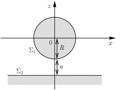
Figure 1: Geometry of the sphere-plate configuration

The geometry of the sphere-plate configuration is illustrated in Fig. 1. It is rotationally symmetric with respect to the $z$ axis, therefore the three dimensional $x_{\mathrm{CM}}$ integration in Eq. (5) trivially reduces to a two dimensional integration. We choose the following order of remaining integrations/summations: first, we do the $T$ integral for each worldline; then, we take the average over all loops, and finally integrate over the resulting energy density. For the first step, the numerically most challenging task is to determine the support $\mathcal{S}_{\ell}$ of $\Theta_{\Sigma}[\mathbf{x}_{\mathrm{CM}}+\sqrt{T}\mathbf{y}_{\ell}]$ on the $T$ axis to perform the $T$ integration in Eq. (15). In the given geometry, $\Theta_{\Sigma}[\mathbf{x}_{\mathrm{CM}}+\sqrt{T}\mathbf{y}_{\ell}]$ equals 1 if there exists a pair $k,l$, such that $\mathbf{x}_{\mathrm{CM}}+\sqrt{T}\mathbf{y}_{\ell k}$ lies inside the sphere and $\mathbf{x}_{\mathrm{CM}}+\sqrt{T}\mathbf{y}_{\ell l}$ lies below the plate; otherwise it is zero. To investigate the support $\mathcal{S}_{\ell}$, it turns out to be useful to distinguish between $\mathbf{x}_{\mathrm{CM}}$ lying inside the sphere, $\mathbf{x}_{\mathrm{CM}}^{2}\leq R^{2}$, and $\mathbf{x}_{\mathrm{CM}}$ lying outside, $\mathbf{x}_{\mathrm{CM}}^{2}>R^{2}$, as the former case is much simpler than the latter.

3.1.1 Inside

Inside the sphere, the support $\mathcal{S}_{\ell}$ is a single $T$ interval. The lower bound $T^{\mathrm{min}}_{\ell}$ is given by the $T$ value at which the loop $\mathbf{x}_{\mathrm{CM}}+\sqrt{T}\mathbf{y}_{\ell}$ touches the plate,

$$T^{\mathrm{min}}_{\ell}=\left(\frac{R+a+x_{\mathrm{CM}z}}{\min_{k}y_{\ell kz}}\right)^{2},$$ (16)

where $\min_{k}y_{\ell kz}$ is the minimal $z$ coordinate of the unit loop $\mathbf{y}_{\ell}$. The upper bound $T^{\mathrm{max}}_{\ell}$ is the largest $T$ value for which the loop intersects the sphere,

$$T^{\mathrm{max}}_{\ell} =\max\Bigl{\{}T:\exists_{k}\bigl{(}\mathbf{x}_{\mathrm{CM}}+\sqrt{T}\mathbf{y}_{\ell k}\bigr{)}^{2}=R^{2}\Bigr{\}}$$ (17)

$$=\max_{k}\left(-{\mathbf{x}_{\mathrm{CM}}\cdot\mathbf{y}_{\ell k}\over\mathbf{y}_{\ell k}^{2}}+\sqrt{\left({\mathbf{x}_{\mathrm{CM}}\cdot\mathbf{y}_{\ell k}\over\mathbf{y}_{\ell k}^{2}}\right)^{2}-{\mathbf{x}_{\mathrm{CM}}^{2}-R^{2}\over\mathbf{y}_{\ell k}^{2}}}\right)^{2}.$$ (18)

Performing the $T$ integration, we obtain the Casimir interaction energy density $\varepsilon_{\text{Casimir}}$ inside the sphere, $E_{\text{Casimir}}=\int d^{3}x_{\text{CM}}\,\varepsilon_{\text{Casimir}}$,

$$\varepsilon_{\text{Casimir}}(\mathbf{x}_{\mathrm{CM}})={1\over 64\pi^{2}}{1\over n_{\mathrm{L}}}\sum_{\ell=1}^{n_{\mathrm{L}}}\biggl{(}\frac{1}{(T^{\mathrm{max}}_{\ell})^{2}}-\frac{1}{(T^{\mathrm{min}}_{\ell})^{2}}\biggr{)}\cdot\theta(T^{\mathrm{max}}_{\ell}-T^{\mathrm{min}}_{\ell}),$$ (19)

where the $\theta$ function takes care of the (non-generic) case that the loop never intersects both surfaces.

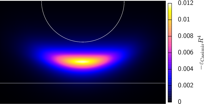
Figure 2: Contour plot of the negative Casimir interaction energy density $\varepsilon_{\text{Casimir}}$ for a sphere of radius $R$ above an infinite plate; the sphere-plate separation $a$ has been chosen as $a=R$ here.

This quantity is plotted in the contour plot Fig. 2 in the region inside the white circle. The contribution to the total Casimir interaction energy is small compared to the energy outside the sphere. The density of the latter is shown in the same figure outside the circle, obtained by the procedure described next.

3.1.2 Outside

Outside the sphere the support $\mathcal{S}_{\ell}$ is not merely one single interval as in the previous case, but a whole set of successive intervals. As illustrated in Fig. 3, for a unit loop $\mathbf{y}_{\ell}$ at a center of mass $\mathbf{x}_{\mathrm{CM}}$ outside the sphere, the ray $\mathbf{x}_{\mathrm{CM}}+\sqrt{T}\mathbf{y}_{\ell k}$ does not pierce the sphere for most indices $k$. The corresponding points on the loop are not relevant for the Casimir energy and the first step in our algorithm is to sort them out. Two conditions are evaluated for this purpose: a point $\mathbf{y}_{\ell k}$ is only relevant for further computations if

1. the vector $\mathbf{y}_{\ell k}$ points towards the sphere, implying

   $$\mathbf{x}_{\mathrm{CM}}\cdot\mathbf{y}_{\ell k}<0,$$ (20)

2. the distance $h$ between the ray $\mathbf{x}_{\mathrm{CM}}+\sqrt{T}\mathbf{y}_{\ell k}$ and the center of the sphere is smaller than the radius $R$,

   $$h^{2}=\mathbf{x}_{\mathrm{CM}}^{2}-\left(\mathbf{x}_{\mathrm{CM}}\cdot{\mathbf{y}_{\ell k}\over|\mathbf{y}_{\ell k}|}\right)^{2}<R^{2}.$$ (21)

If these conditions are fulfilled, the $T$ values at which the ray intersects the sphere are determined by

$$(\mathbf{x}_{\mathrm{CM}}+\sqrt{T}\mathbf{y}_{\ell k})^{2}=R^{2},$$ (22)

which has the solutions

$$T^{\pm}_{\ell k}=\left(-{\mathbf{x}_{\mathrm{CM}}\cdot\mathbf{y}_{\ell k}\over\mathbf{y}_{\ell k}^{2}}\pm\sqrt{\left({\mathbf{x}_{\mathrm{CM}}\cdot\mathbf{y}_{\ell k}\over\mathbf{y}_{\ell k}^{2}}\right)^{2}-{\mathbf{x}_{\mathrm{CM}}^{2}-R^{2}\over\mathbf{y}_{\ell k}^{2}}}\right)^{2}.$$ (23)

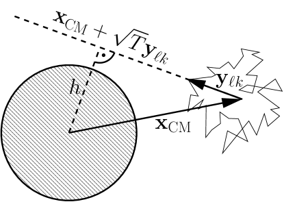
Figure 3: For any propertime $T$, the ray $\mathbf{x}_{\mathrm{CM}}+\sqrt{T}\mathbf{y}_{\ell k}$ does not intersect the sphere. The corresponding point $\mathbf{y}_{\ell l}$ is thus not relevant for the interaction energy density at the given $\mathbf{x}_{\text{CM}}$ and consequently sorted out in a first step of the algorithm.

For $T\in[T_{\ell k}^{-},T_{\ell k}^{+}]$ the point $\mathbf{x}_{\mathrm{CM}}+\sqrt{T}\mathbf{y}_{\ell k}$ lies inside the sphere and consequently we know that the loop intersects the sphere. For a given loop, the total set of $T$ values for which this is the case is the union of the intervals $[T_{\ell k}^{-},T_{\ell k}^{+}]$ of all points $y_{\ell k}$ in the unit loop, $\bigcup_{k}[T_{\ell k}^{-},T_{\ell k}^{+}]$. Taking into account the minimal $T$ value for which the loop intersects the plate, $T^{\mathrm{min}}_{\ell}$, the contribution of the unit loop to the propertime integrand has the support

$$\mathcal{S}_{\ell}=[T^{\mathrm{min}}_{\ell},\infty)\cap\bigcup_{k}[T_{\ell k}^{-},T_{\ell k}^{+}].$$ (24)

The set union can be determined efficiently by use of a sorting algorithm like quicksort, for example. Once $\mathcal{S}_{\ell}$ is determined, the $T$ integration can be performed analytically. The worldline estimate for the Casimir interaction energy density outside the sphere therewith is

$$\varepsilon_{\text{Casimir}}(\mathbf{x}_{\mathrm{CM}})=-{1\over 32\pi^{2}}{1\over n_{\mathrm{L}}}\sum_{\ell=1}^{n_{\mathrm{L}}}\int_{\mathcal{S}_{\ell}}{dT\over T^{3}},$$ (25)

which is plotted in Fig. 2 outside the white circle.

3.1.3 Optimization

The algorithm so far works well if the distance between sphere and plate $a$ is of the same order of magnitude as the sphere’s radius $R$, $a\approx R$. To improve the accuracy by increasing the number of loops $n_{\mathrm{L}}$ and the number of points per loop $N$, the algorithm can be parallelized as embarrassingly parallel computation by dividing the loop ensemble into independently processed sub-ensembles. However, if the two scales $a$ and $R$ differ significantly in size, additional improvements of our algorithm are advisable.

Large distances ($a\gg R$): if the distance $a$ is large compared to the radius $R$, the algorithm described so far becomes inefficient due to the following reason: only loops with a minimal extent of the same order of magnitude as the distance between sphere and plate do contribute to the Casimir energy. For a loop $\mathbf{x}_{\mathrm{CM}}+\sqrt{T}\mathbf{y}_{\ell}$ this means, that the unit loop $\mathbf{y}_{\ell}$ has to be scaled by a large factor $\sqrt{T}$. This implies that the distance between subsequent points on the loop increases, too. However, to ensure that the scaled loops still resolve the sphere, this distance should be significantly smaller than the sphere’s radius. Thus, the number of points per loop $N$ has to be increased with increasing $a/R$.

A rough measure for the extent of a loop is the variance of the coordinates of its points. The ensemble average of the variance for large $N$ is $\langle(\sqrt{T}\mathbf{y}_{\ell k})^{2}\rangle=T/6$. As a consequence we expect the $T$ integral to be dominated by $T\approx 6a^{2}$, also because the contribution for large $T$ is damped by the $1/T^{3}$ factor. The root-mean-square of the distance between two subsequent points on a loop for large $N$ is $\sigma=\sqrt{2T/N}$. Using the dominating $T$ value we obtain $\sigma\approx 2\sqrt{3/N}a$. We demand this value to be much smaller than the radius of the sphere, which implies $N\gg 12a^{2}/R^{2}$. For a distance $a=10R$, already much more than 1000 ppl have to be used, for $a=100R$ much more than 100 000 ppl.

A slight modification enables our algorithm to cope with this high resolution and the corresponding amount of data much more efficiently. So far, for all center of masses $\mathbf{x}_{\mathrm{CM}}$ with a common $z$ coordinate $\mathbf{x}_{\mathrm{CM}z}$, the first interval on the right-hand side of Eq. (24), $[T^{\mathrm{min}}_{\ell},\infty)$, is the same, which can be utilized to speed up the calculation. In contrast, the union in the same equation is different for all centers of masses. However, it is this part of the equation which consumes most of the CPU time. Modifying the transformation Eq. (14) reverses the circumstances: let us define the rotation $R(\mathbf{x}_{\mathrm{CM}},\mathbf{e}_{z})$ by $\mathbf{x}_{\mathrm{CM}}/|\mathbf{x}_{\mathrm{CM}}|=R(\mathbf{x}_{\mathrm{CM}},\mathbf{e}_{z})\mathbf{e}_{z}$. By using

$$\mathbf{x}_{\ell k}=\mathbf{x}_{\mathrm{CM}}+\sqrt{T}R(\mathbf{x}_{\mathrm{CM}},\mathbf{e}_{z})\mathbf{y}_{\ell k}$$ (26)

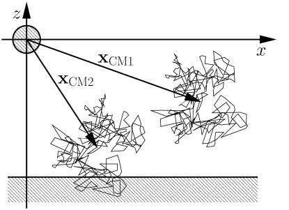
Figure 4: Sketch of a unit loop at different centers of masses $x_{\mathrm{CM}1}$ and $x_{\mathrm{CM}2}$, as used for large $a/R$. The unit loop is rotated corresponding to the orientation of the center of mass.

(see Fig. 4), the union in Eq. (24) is the same for all center-of-mass values $x_{\mathrm{CM}}$ with a given absolute value $|\mathbf{x}_{\mathrm{CM}}|$ and can be computed once and for all. In turn, $T^{\mathrm{min}}_{\ell}$ is no longer degenerate with respect to some $\mathbf{x}_{\text{CM}}$ coordinate. The important advantage is that this dependence can be computed much faster. For each loop, we generate an array of its minimal $z$ coordinate as function of the angle between $\mathbf{x}_{\mathrm{CM}}$ and $\mathbf{e}_{z}$. The bound $T^{\mathrm{min}}_{\ell}$ then results from Eq. (16), where the minimum is read from the array. Note that the transformation (26) is a legitimate symmetry operation for ensemble-averaged quantities, owing to the rotational invariance of the exponential weight factor in Eq. (13).

There is a price to be paid for the desired feature of having a common set union in Eq. (24) for different centers of masses $x_{\mathrm{CM}}$: without the transformation, all points of a given unit loop are equally involved in scanning the curvature of the sphere. With the transformation, always the same points of a unit loop are close to the sphere, independently of $\mathbf{x}_{\text{CM}}$. This corresponds to a loss of statistics, implying a slight increase of the statistical errors. However, this is by far compensated for by the gain in computation speed, which enables us to significantly reduce again the statistical error by brute force.

Small distances ($a\ll R$): the main contribution of the Casimir interaction energy density is localized between sphere and plate. If the distance $a$ is much smaller than the sphere’s radius $R$, the lower bound of the support $\mathcal{S}_{\ell}$ in that region is at very small $T$ values compared to the upper bound of the support’s first interval. Since the $T$ integrand falls off rapidly with $1/T^{3}$, the $T$ integral is dominated by this lower bound. Therefore, a very good estimate is given by replacing $\mathcal{S}_{\ell}$ simply by the interval $[T_{\ell}^{\text{min}},\infty)$, resulting in

$$\varepsilon_{\text{Casimir}}(x_{\mathrm{CM}})\simeq-{1\over 64\pi^{2}}{1\over n_{\mathrm{L}}}\sum_{\ell=1}^{n_{\mathrm{L}}}{1\over(T_{\ell}^{\text{min}})^{2}}.$$ (27)

In particular outside the sphere, the numerical evaluation of this expression is much faster than the evaluation of the full expression Eq. (25).

For a rough estimate of the validity range of this approximation, we use the ensemble’s standard deviation of the point position, ${\langle(\sqrt{T}\mathbf{y}_{\ell k})^{2}\rangle}={T/6}$, to estimate the extent of a loop. Right between sphere and plate, where the energy density is largest, the lower bound of the propertime integral then is approximately $T_{\ell}^{\text{min}}\approx 3a^{2}/2$. If the extent of the loop increases beyond $a/2+2R$, we expect the loop to intersect the sphere no longer for $T_{1}\gtrapprox 6(a/2+2R)^{2}$. By setting the value of $T_{1}$ to infinity instead, as done in Eq. (27), we introduce a systematic error $\Delta\varepsilon_{\text{Casimir}}/\varepsilon_{\text{Casimir}}\lessapprox\bigl{(}1+4R/a\bigr{)}^{-4}$. For distances $a$ smaller than $0.8R$ this error is smaller than one per mille. In this work, we have used Eq. (27) to compute high-precision values for $a<0.02R$.

3.1.4 Results

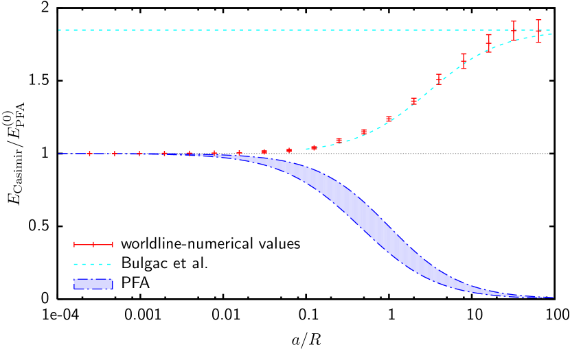
Figure 5: Casimir interaction energy of a sphere with radius $R$ and an infinite plate vs. the curvature parameter $a/R$. The energy is normalized to the zeroth-order PFA formula (2), $E^{(0)}_{\text{PFA}}$. For larger curvature parameter, the PFA estimate (dot-dashed line) differs qualitatively from the worldline result (crosses with error bars). Here, we observe good agreement of our result with the exact solution of [28] which is available for $a/R\gtrsim 0.1$ (dashed line).

Figure 5 presents a global view on the Casimir interaction energy for a wide range of the curvature parameter $a/R$; the energy is normalized to the zeroth order of the PFA formula (2), $E^{(0)}_{\text{PFA}}$. For small $a/R$ (“large spheres”), our worldline result (crosses with error bars) and the full sphere- and plate-based PFA estimates (dashed-dotted lines) show reasonable agreement, settling at the zeroth-order PFA $E^{(0)}_{\text{PFA}}$. The full PFA departs on the percent level from $E^{(0)}_{\text{PFA}}$ for $a/R\gtrsim 0.01$, exhibiting a relative energy decrease. By contrast, our worldline result first stays close to $E^{(0)}_{\text{PFA}}$ and then increases towards larger energy values relative to $E^{(0)}_{\text{PFA}}$. This observation confirms earlier worldline studies [26] and agrees with the optical approximation [27] in this curvature regime.

For larger curvature $a/R\gtrsim 0.1$ (“smaller spheres”), we observe a strong increase relative to $E^{(0)}_{\text{PFA}}$ [33]. Here, our data satisfactorily agrees with the exact solution found recently for this regime [28] (dashed line). The latter work also provides for an exact asymptotic limit for $a/R\to\infty$, resulting in $180/\pi^{4}$ for our normalization. Our worldline data confirms this limit in Fig. 5.

Two important lessons can be learned from this plot: first, the PFA already fails to predict the correct sign of the curvature effects beyond zeroth order, see also [40]. Second, the relation between the Casimir effect for Dirichlet scalars and that for the EM field is strongly geometry dependent. For the parallel-plate case, Casimir forces only differ by the number of degrees of freedom, cf. the coefficient $c_{\text{PP}}$ in Eq. (2). For large curvature, the Casimir energy for the Dirichlet scalar scales with $a^{-2}$, whereas that for the EM field obeys the Casimir-Polder law $\sim a^{-4}$ [41, 42]. Already this difference demonstrates that simple approximation methods such as the PFA are highly problematic, since no reference to the nature of the fluctuating field other than the coefficient $c_{\text{PP}}$ is made.

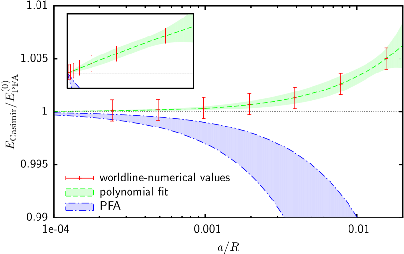
Figure 6: Magnified view of Fig. 5 for small $a/R$. The 0.1% validity range of the PFA is characterized by curvature parameters, where the error band of our worldline results and the PFA band (blue-shaded/in between the dot-dashed lines) overlap, see Eq. (28). The dashed line depicts a constraint polynomial fit of the worldline result, $p(a/R)=1+0.35(a/R)-1.92(a/R)^{2}$, and its standard deviation, see Eq. (30). The inlay displays the same curves with a linear $a/R$ axis.

For a quantitative determination of the PFA validity limits, Fig. 6 displays the zeroth-order normalized energy for small curvature parameter $a/R$. Here, our result has an accuracy of 0.1% (jack-knife analysis). The error is dominated by the Monte Carlo sampling and the ordinary-integration accuracy; the error from the worldline discretization is found negligible in this regime, implying a sufficient proximity to the continuum limit.

In addition to our numerical error band, we consider the region between the sphere- and the plate-based PFA as the PFA error band. We identify the 0.1% accuracy limit of the PFA with the curvature parameter $a/R|_{0.1\%}$ where the two bands do no longer overlap. We obtain

$$\frac{a}{R}\Big{|}^{\text{PFA}}_{0.1\%}\leq 0.00073$$ (28)

as the corresponding validity range for the curvature parameter. For instance, for a typical sphere with $R=200\mu$m and an experimental accuracy goal of $0.1\%$, the PFA should not be used for $a\gtrsim 150$nm. We conclude that the PFA should be dropped from the analysis of future experiments.

For the 1% accuracy limit of the PFA, we increase the band of our worldline estimate by this size and again determine the curvature parameter for which there is no intersection with the PFA band anymore. We obtain

$$\frac{a}{R}\Big{|}^{\text{PFA}}_{1\%}\leq 0.00755.$$ (29)

For a sphere with $R=200\mu$m and an experimental accuracy goal of $1\%$, the PFA holds for $a<1.5\mu$m. This result confirms the use of the PFA for the data analysis of the corresponding experiments performed so far.

In order to study the asymptotic expansion of the normalized energy, we fit our worldline numerical data to a second-order polynomial for $a/R<0.1$ and include the exactly known result for $a/R\to 0$. We obtain

$$E^{\text{sphere-plate}}_{\text{WN data fit}}=-c_{\text{PP}}\frac{\pi^{3}}{1440}\frac{R}{a^{2}}\left(1+0.35\frac{a}{R}-1.92\frac{a^{2}}{R^{2}}\pm 0.19\frac{a}{R}\sqrt{1-137.2\frac{a}{R}+5125\frac{a^{2}}{R^{2}}}\right),$$ (30)

valid for $a/R<0.1$; here, $c_{\text{PP}}=1$ for the real and $c_{\text{PP}}=2$ for a complex Dirichlet scalar. The fit result is plotted in Fig. 6 (dashed lines), which illustrates that $E\simeq E_{\text{WN data fit}}$ is a satisfactory approximation to the Casimir energy for $a/R<0.1$, replacing the PFA (2). The inlay of Figure 6 displays the same curves with a linear $a/R$ axis, illustrating that the lowest-order curvature effect is linear in $a/R$. A more direct result for the linear curvature coefficient can be obtained by a constraint linear fit; in this simpler case, the fit polynomial yields $p_{\text{fit}}(a/R)=1+(0.33\pm 0.06)\frac{a}{R}$ instead of the expression in parentheses in Eq. (30). Given the results of the PFA (2), the semiclassical approximation [24], $p_{sc}(a/R)\simeq 1-0.17\frac{a}{R}$, cf. [28], and the optical approximation [27], $p_{opt}(a/R)\simeq 1+0.05\frac{a}{R}$, the latter appears to estimate curvature effects more appropriately; but all these approximations are not quantitatively reliable for beyond-zeroth-order curvature effects.

3.2 Cylinder above plate

The cylinder-plate configuration is a promising tool for high-precision experiments [43], since the force signal increases linearly with the cylinder length. The numerics is very similar to the sphere-plate configuration, even less computing power is required, because only two dimensional loops have to be processed due to the translational symmetry. Figure 7 shows the corresponding Casimir interaction energy versus the curvature parameter. The energy axis is again normalized to the zeroth-order PFA result,

$$E_{\text{PFA}}^{(0)}(a,R)=-c_{\text{PP}}\frac{\pi^{3}}{1920\sqrt{2}}\,\,\frac{R^{1/2}}{a^{5/2}}.$$ (31)

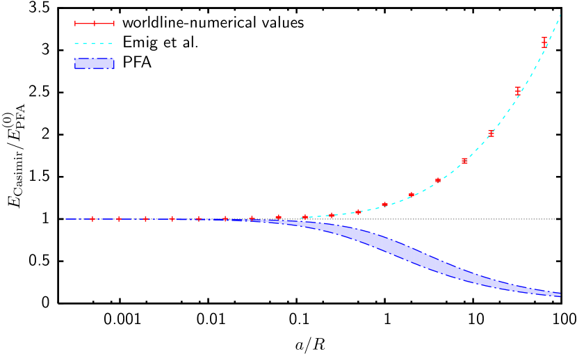
Figure 7: Casimir interaction energy (normalized to $E_{\text{PFA}}^{(0)}$) of an infinitely long cylinder with radius $R$ at a distance $a$ above an infinite plate vs. the curvature parameter $a/R$. We observe good agreement of our result with the exact solution of [29] which is available for $a/R\gtrsim 0.1$ (dashed line).

A magnified view of the small curvature region in Fig. 7 is shown in Fig. 8. As for the sphere-plate configuration, we fit our data to a second-order polynomial in this range, including the exactly known result for $a/R\to 0$, yielding

$$E^{\text{cylinder-plate}}_{\text{WN data fit}}\!=-\frac{c_{\text{PP}}\pi^{3}}{1920\sqrt{2}}\,\frac{R^{1/2}}{a^{5/2}}\left(\!1+0.21\frac{a}{R}-0.66\frac{a^{2}}{R^{2}}\pm 0.097\frac{a}{R}\sqrt{1-68.60\frac{a}{R}+1282\frac{a^{2}}{R^{2}}}\right),$$ (32)

for ${a}/{R}<0.1$. The inlay of Fig. 8 shows the same data with a linear $a/R$ axis. As for the sphere-plate geometry, this plot demonstrates that the lowest-order curvature effect is linear in $a/R$. A simpler linear fit to our data results in $p_{\text{fit}}(x)\simeq 1+(0.195\pm 0.028)\frac{a}{R}$. This is in remarkable agreement with the recently found analytical result $p(a/R)=1+0.19\bar{4}\frac{a}{R}+\mathcal{O}(a^{2}/R^{2})$ [30], which represents a strong confirmation for both methods.

The qualitative conclusions for the validity of the PFA are similar to that for the sphere above a plate: beyond leading order, the PFA even predicts the wrong sign of the curvature effects. Quantitatively, the PFA validity limits are a factor $\sim 3$ larger than Eqs. (28),(29), owing to the absence of curvature along the cylinder axis.

The most important difference to the sphere-plate case arises for large $a/R$. Here, the data is compatible with a log-like increase relative to $E_{\text{PFA}}^{(0)}$, implying a surprisingly weak decrease of the Casimir force for large curvature $a/R\to\infty$. Our result agrees nicely with the recent exact result [29] which is available for $a/R\gtrsim 0.1$. The data thus confirms the observation of [29] that the resulting Casimir force has the weakest possible decay, $F\sim 1/[a^{3}\ln(a/R)]$, for asymptotically large curvature parameter $a/R\to\infty$.

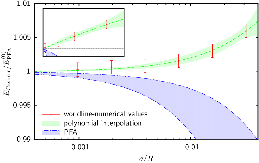
Figure 8: Magnified view of Fig. 7 for small values of $a/R$. The dashed line with error band depicts a constraint polynomial fit to the numerical data, $p(a/R)=1+0.21(a/R)-0.66(a/R)^{2}$, and its standard deviation. The inlay displays the same curves with a linear $a/R$ axis.

3.3 Parallel plates revisited

Figure 9: Geometry of Casimir’s parallel-plate configuration. A loop contributes to the Casimir interaction energy if its extent $L_{\ell}$ along the $z$ direction is larger than the plate distance $a$.

As discussed at the beginning of this section, the order of the $T$ and $\mathbf{x}_{\text{CM}}$ integration and the ensemble averaging can be chosen arbitrarily. As an example for an “unusual” order, let us reconsider Casimir’s classic parallel-plate configuration in $D=d+1$ dimensional spacetime, doing the $\mathbf{x}_{\text{CM}}$ integral first and keeping the ensemble average till the very end. This will reveal an unexpected mapping between the $D$-dimensional Casimir effect and standard polymer physics.

In $d$ space dimensions, the surface or area volume $A$ of the Casimir plates is taken as $d-1$ dimensional. The two (hyper-)plates are separated by a distance $a$ along the $z$ direction which is normal to the plates, see Fig. 9. For this configuration, the Casimir interaction energy for the massless Dirichlet scalar boils down to

$$E_{\text{Casimir}}=-A\,\frac{1}{2(4\pi)^{D/2}}\frac{1}{n_{\text{L}}}\sum_{\ell=1}^{n_{\text{L}}}\int_{0}^{\infty}\frac{dT}{T^{1+D/2}}\,\int^{\infty}_{-\infty}\,dz_{\text{CM}}\,\Theta[z_{\text{CM}}+\sqrt{T}y_{z\ell}],$$ (33)

where $y_{z\ell}$ denotes the $z$ coordinate of the $\ell$th unit loop. Let us denote the extent of the $\ell$th unit loop in the $z$ direction by $L_{\ell}$,

$$L_{\ell}:=\max_{i,\,k}\left(|y_{z\ell i}-y_{z\ell k}|\right),$$ (34)

see Fig. 9. A scaled unit loop intersects both plates if $\sqrt{T}L_{\ell}\geq a$. For a given unit loop with extent $L_{\ell}$ and for a given propertime value $T$, the support of the $z_{\text{CM}}$ integral corresponds to an interval $I_{z}(T,L_{\ell})=\sqrt{T}L_{\ell}-a$. Independently of the precise location of this interval on the $z_{\text{CM}}$ axis, the $z_{\text{CM}}$ integral yields,

$$\int_{-\infty}^{\infty}\,dz_{\text{CM}}\,\Theta[z_{\text{CM}}+\sqrt{T}y_{z\ell}]=(\sqrt{T}L_{\ell}-a)\,\theta(\sqrt{T}L_{\ell}-a).$$ (35)

Now, also the $T$ integral can be done analytically, resulting in

$$E_{\text{Casimir}} = -\frac{A}{a^{D-1}}\,\frac{1}{D(D-1)(4\pi)^{D/2}}\frac{1}{n_{\text{L}}}\sum_{\ell=1}^{n_{\text{L}}}L_{\ell}^{D}$$ (36)

$$= -\frac{A}{a^{D-1}}\,\frac{1}{D(D-1)(4\pi)^{D/2}}\langle L_{\ell}^{D}\,\rangle.$$

We observe that the Casimir interaction energy of the parallel-plate configuration in $D=d+1$ spacetime dimensions is proportional to the $D$th moment of the ensemble-averaged extent of a unit loop. This ensemble average could easily be performed, which would lead us back to the results of [26].

Here, we will be satisfied by hilighting Eq. (36) from a different perspective, namely, in the language of polymer physics. The Gaußian velocity distribution of our worldlines is identical to the Hamiltonian of a polymer, i.e., the continuum limit of a random chain, without self-avoidance or excluded-volume effect [44] in the limit of zero end-to-end distance. In this language, $L_{\ell}$ corresponds to the maximum spatial extent of the closed polymer measured in units of $\sqrt{l_{\text{p}}c/(2D_{\text{p}})}$. Here, $l_{\text{p}}=Nc$ denotes the total length of the polymer, $c$ is the chain length, and $D_{\text{p}}$ is the number of dimensions in which the polymer can move; the latter is completely arbitrary and independent of the dimensionality of the Casimir system. Since $L_{\ell}$ is a highly nonlocal object, its ensemble average is actually not so easily computable by standard methods. Our result Eq. (36) now maps the problem of computing any $D$th moment of $L_{\ell}$ on the $D$-dimensional Casimir problem for parallel plates. Using the standard result for the latter [45],

$$E_{\text{Casimir}}=-\frac{A}{a^{D-1}}\,\frac{1}{(4\pi)^{D/2}}\,\Gamma(D/2)\,\zeta(D),$$ (37)

we obtain by comparison with Eq. (36),

$$\langle L_{\ell}^{D}[y]\rangle=D(D-1)\,\Gamma(D/2)\,\zeta(D),$$ (38)

a result that we have so far not been able to find in the literature of polymer physics. Even the limit $D\to 1$ can be taken, corresponding to the Casimir effect in zero space dimensions: this results in $\langle L_{\ell}[y]\rangle=\sqrt{\pi}$ for the average extent of a closed polymer.

4 Conclusions

We have presented improved worldline numerical algorithms that can efficiently deal with Casimir configurations involving curved surfaces. We have used these algorithms to compute Casimir interaction energies for the sphere-plate and cylinder-plate configuration induced by a scalar field with Dirichlet boundary conditions. These computations are done from first principles for a wide range of curvature parameters $a/R$. In general, we observe that curvature effects and geometry dependencies are intriguingly rich, implying that naive estimates can easily be misguiding. In particular, predictions based on the PFA are only reliable in the asymptotic no-curvature limit with quantitative validity bounds given above. We have constructed polynomial fits of our results which can be used in the small-curvature regime, $a/R\lesssim 0.1$, as a well-founded substitute for the PFA formulas. Given the size of the true curvature corrections for the Dirichlet scalar, we expect that genuine Casimir curvature effects are in reach of currently planned experiments. In this spirit, the so-called lateral Casimir force for corrugated surfaces has recently been proposed as a suitable candidate for identifying non-trivial geometry dependences beyond the PFA [46].

Beyond the Dirichlet scalar investigated here, it is well possible, e.g., for the EM field, that some cancellation of curvature effects occurs between modes obeying different boundary conditions. In fact, such a partial cancellation between TE and TM modes of the separable cylinder-plate geometry can be observed in the recent exact result for the EM field for medium curvature [29]; for small curvature, curvature effects can even reverse sign [30]. More quantitatively, the TM mode in the cylinder-plate case obeys Dirichlet boundary condition and thus contributes, e.g., to the linear curvature correction with a coefficient $\simeq 0.194$, as discussed below Eq. (32); the TE mode obeys Neumann boundary conditions, giving a negative contribution which in total turns this linear coefficient for the EM field into $\simeq-0.48$ [30]. The latter result, in fact, lies in the broad range of $[-0.92,-0.25]$ spanned by the PFA; since the PFA does not make any reference to the nature of the fluctuating field, this rough coincidence is, of course, purely accidental. This strong dependence of Casimir curvature effects on the nature of the fluctuating fields alone demonstrates already that approximations ignoring this difference such as the PFA cannot be trusted. We emphasize again that Casimir calculations for the EM field in non-separable geometries, such as the important sphere-plate case, remain a prominent open problem.

From a technical point of view, we would like to stress that our results demonstrate the capability of worldline numerics for performing high-precision computations with comparatively little computing power. The simple scalability of the algorithms and the flexibility for adapting them to arbitrary geometries makes worldline numerics a unique tool for computing quantum energies.

Our algorithmic strategies also revealed an unexpected mapping between the $D$-dimensional parallel-plate Casimir effect and aspects of a random-chain polymer ensemble. The origin of this mapping, of course, lies in the fact that both quantum fluctuations in Casimir systems as well as a polymer ensemble can be described by Feynman path integrals. In the present case, the mapping can be utilized to transform a comparatively difficult polymer problem into a field-theoretic Casimir problem which can be solved by a variety of techniques. We believe that this mapping is just a special case of a more general class of mappings with potentially fruitful applications in both directions.

References

- [1] H.B.G. Casimir, Kon. Ned. Akad. Wetensch. Proc. 51, 793 (1948).
- [2] S. K. Lamoreaux, Phys. Rev. Lett. 78, 5 (1997).
- [3] U. Mohideen and A. Roy, Phys. Rev. Lett. 81, 4549 (1998);
- [4] A. Roy, C. Y. Lin and U. Mohideen, Phys. Rev. D 60, 111101 (1999).
- [5] T. Ederth, Phys. Rev. A 62, 062104 (2000)
- [6] H.B. Chan, V.A. Aksyuk, R.N. Kleiman, D.J. Bishop and F. Capasso, Science 291, 1941 (2001).
- [7] F. Chen, U. Mohideen, G.L. Klimchitskaya and V.M. Mostepanenko, Phys. Rev. Lett. 88, 101801 (2002).
- [8] M. Bordag, B. Geyer, G. L. Klimchitskaya and V. M. Mostepanenko, Phys. Rev. D 58, 075003 (1998), ibid. 60, 055004 (1999), ibid. 62, 011701 (2000).
- [9] J. C. Long, H. W. Chan and J. C. Price, Nucl. Phys. B 539, 23 (1999).
- [10] V. M. Mostepanenko and M. Novello, Phys. Rev. D 63, 115003 (2001).
- [11] K. A. Milton, R. Kantowski, C. Kao and Y. Wang, Mod. Phys. Lett. A 16, 2281 (2001).
- [12] R.S. Decca, E. Fischbach, G.L. Klimchitskaya, D.E. Krause, D.L. Lopez and V.M. Mostepanenko, Phys. Rev. D 68, 116003 (2003), R.S. Decca, D. Lopez, H.B. Chan, E. Fischbach, D.E. Krause and C.R. Jamell, Phys. Rev. Lett. 94, 240401 (2005).
- [13] G.L. Klimchitskaya, A. Roy, U. Mohideen, and V.M. Mostepanenko, Phys. Rev. A 60, 3487 (1999).
- [14] A. Lambrecht and S. Reynaud, Eur. Phys. J. D 8, 309 (2000).
- [15] V.B. Bezerra, G.L. Klimchitskaya, and V.M. Mostepanenko, Phys. Rev. A 62, 014102 (2000).
- [16] M. Bordag, U. Mohideen and V. M. Mostepanenko, Phys. Rept. 353, 1 (2001).
- [17] P.A. Maia Neto, A. Lambrecht, and S. Reynaud, Europhys. Lett. 69, 924 (2005); Phys. Rev. A 72, 012115 (2005).
- [18] V. M. Mostepanenko et al., arXiv:quant-ph/0512134.
- [19] I. Brevik, S. A. Ellingsen and K. A. Milton, arXiv:quant-ph/0605005.
- [20] M. Boström and Bo E. Sernelius, Phys. Rev. Lett. 84, 4757 (2000).
- [21] N. Graham, R. L. Jaffe, V. Khemani, M. Quandt, M. Scandurra and H. Weigel, Nucl. Phys. B 645, 49 (2002).
- [22] G. Bressi, G. Carugno, R. Onofrio and G. Ruoso, Phys. Rev. Lett. 88, 041804 (2002).
- [23] B.V. Derjaguin, I.I. Abrikosova, E.M. Lifshitz, Q.Rev. 10, 295 (1956); J. Blocki, J. Randrup, W.J. Swiatecki, C.F. Tsang, Ann. Phys. (N.Y.) 105, 427 (1977).
- [24] M. Schaden and L. Spruch, Phys. Rev. A 58, 935 (1998); Phys. Rev. Lett. 84 459 (2000)
- [25] R. Golestanian and M. Kardar, Phys. Rev. A 58, 1713 (1998); T. Emig, A. Hanke and M. Kardar, Phys. Rev. Lett. 87 (2001) 260402; T. Emig and R. Buscher, Nucl. Phys. B 696, 468 (2004).
- [26] H. Gies, K. Langfeld and L. Moyaerts, JHEP 0306, 018 (2003); arXiv:hep-th/0311168.
- [27] A. Scardicchio and R. L. Jaffe, Nucl. Phys. B 704, 552 (2005); Phys. Rev. Lett. 92, 070402 (2004).
- [28] A. Bulgac, P. Magierski and A. Wirzba, Phys. Rev. D 73, 025007 (2006) [arXiv:hep-th/0511056]; A. Wirzba, A. Bulgac and P. Magierski, J. Phys. A 39 (2006) 6815 [arXiv:quant-ph/0511057].
- [29] T. Emig, R. L. Jaffe, M. Kardar and A. Scardicchio, Phys. Rev. Lett. 96 (2006) 080403 [arXiv:cond-mat/0601055].
- [30] M. Bordag, arXiv:hep-th/0602295.
- [31] H. Gies and K. Langfeld, Nucl. Phys. B 613, 353 (2001); Int. J. Mod. Phys. A 17, 966 (2002).
- [32] see, e.g., C. Schubert, Phys. Rept. 355, 73 (2001).
- [33] H. Gies and K. Klingmuller, J. Phys. A 39 6415 (2006) [arXiv:hep-th/0511092].
- [34] H. Gies and K. Klingmuller, arXiv:quant-ph/0601094, to appear in Phys. Rev. Lett. (2006).
- [35] D. Deutsch and P. Candelas, Phys. Rev. D 20, 3063 (1979); P. Candelas, Annals Phys. 143, 241 (1982).
- [36] G. Barton, J. Phys. A 34, 4083 (2001).
- [37] N. Graham, R. L. Jaffe, V. Khemani, M. Quandt, O. Schroeder and H. Weigel, Nucl. Phys. B 677, 379 (2004) [arXiv:hep-th/0309130]; H. Weigel, arXiv:hep-th/0310301.
- [38] O. Kenneth and I. Klich, arXiv:quant-ph/0601011.
- [39] A. Scardicchio and R. L. Jaffe, Nucl. Phys. B 743 (2006) 249 [arXiv:quant-ph/0507042].
- [40] I. Brevik, E.K. Dahl and G.O. Myhr, J. Phys. A 38, L49 (2005).
- [41] H.B.G. Casimir and D. Polder, Phys. Rev. 73, 360 (1948).
- [42] V. Druzhinina and M. DeKieviet, Phys. Rev. Lett. 91, 193202 (2003).
- [43] M. Brown-Hayes, D.A.R. Dalvit, F.D. Mazzitelli, W.J. Kim and R. Onofrio, Phys. Rev. A 72, 052102 (2005).
- [44] H. Kleinert, “PATH INTEGRALS in Quantum Mechanics, Statistics, Polymer Physics, and Financial Markets ,” World Scientific, Singapore (2004).
- [45] H. Verschelde, L. Wille and P. Phariseau, Phys. Lett. B 149, 396 (1984); N. F. Svaiter and B. F. Svaiter, J. Math. Phys. 32, 175 (1991).
- [46] R. B. Rodrigues, P. A. Maia Neto, A. Lambrecht and S. Reynaud, Phys. Rev. Lett. 96, 100402 (2006) [arXiv:quant-ph/0603120].