Minimum uncertainty measurements of angle and angular momentum

Abstract

The uncertainty relations for angle and angular momentum are revisited. We use the exponential of the angle instead of the angle itself and adopt dispersion as a natural measure of resolution. We find states that minimize the uncertainty product under the constraint of a given uncertainty in angle or in angular momentum. These states are described in terms of Mathieu wave functions and may be approximated by a von Mises distribution, which is the closest analogous of the Gaussian on the unit circle. We report experimental results using beam optics that confirm our predictions.

Light carries and transfers energy as well as linear and angular momentum. The angular momentum contains a spin contribution, associated with polarization, and an orbital component, linked with the spatial profile of the light intensity and phase ABP2003 .

The seminal paper of Allen et al ABSW1992 firmly establishes that the Laguerre-Gauss modes, typical of cylindrical symmetry, carry a well-defined angular momentum per photon. In the paraxial limit, this orbital component is polarization independent and arises solely from the azimuthal phase dependence $e^{im\phi}$, which gives rise to spiral wave fronts. The index $m$ takes only integer values and can be seen as the eigenvalue of the orbital angular momentum operator. In consequence, the Laguerre-Gauss modes constitute a complete set and can be used to represent quantum photon states EN1992 ; Wun2004 ; CPB2005 .

The possibility of exploiting these light fields for driving micromachines, and their applications as optical tweezers and traps, have attracted a good deal of attention SDAP1997 ; GO2001 ; PMA2001 . Moreover, entangled photons prepared in a superposition of states bearing a well-defined orbital angular momentum provide access to multidimensional entanglement. This is of considerable importance in quantum information and cryptography because with these states more information can be stored and there is less sensitivity to decoherence MVWZ2001 ; MTT2002 ; VPJ2003 ; MVRH2004 ; AOEW2005 .

Recently, by precise measurements on a light beam, an experimental test of the uncertainty principle for angle and angular momentum has been demonstrated FBY2004 ; PBZ2005 . The idea is to pass the beam through an angular aperture and measure the resulting distribution of angular-momentum states LPB2002 . Moreover, one can even identify the form of the aperture that corresponds to the minimum uncertainty states for these variables.

In the following, we deal with cylindrical symmetry; we are concerned with the planar rotations by an angle $\phi$ in the plane $x$-$y$, generated by the angular momentum along the $z$ axis, which for simplicity will be denoted henceforth as $\hat{L}$. In this respect, we recall that the proper definition of angular variables in quantum mechanics is beset by well-known difficulties PLP1998 ; LS2000 . For the case of a harmonic oscillator, the problems essentially arise from two basic sources: the periodicity and the semiboundedness of the energy spectrum. The first prevents the existence of a phase operator in the infinite-dimensional Hilbert space, but not of its exponential. The second entails that this exponential is not unitary.

Although we have here the same kind of problems linked with the periodicity, the angular momentum has a spectrum that includes both positive and negative integers, which allows us to introduce a well behaved exponential of the angle operator, denoted by $\hat{E}$ LS1998 . Since the angle is canonically conjugate to $\hat{L}$, we start from the commutation relation LS2000

$$[\hat{E},\hat{L}]=\hat{E}.$$ (1)

The goal of this Letter is precisely to develop a comprehensive approach to the minimum uncertainty states associated with the relation (1). Our results will corroborate that the use of $E$ provides a good description of the angular behavior and the associated minimum uncertainty states turn out to be Mathieu beams in wave optics. This will establish a proper basis for information processing with these conjugate variables.

We also stress that, since angle is $2\pi$ periodic, the corresponding quantum statistical description should also preserve this periodicity. Provided that a non-periodic measure of the angular spread is used, as for example the variance, such a resolution depends on the $2\pi$ window chosen. To prevent this, we recall that another appropriate and meaningful measure of angular spread is the dispersion Rao1965

$$D^{2}=1-|\langle e^{i\phi}\rangle|^{2}.$$ (2)

Here

$$\langle e^{i\phi}\rangle=\int_{0}^{2\pi}d\phi\ P(\phi)\ e^{i\phi}$$ (3)

and $P(\phi)$ is the angle distribution. As expected, it possesses all the good properties: it is periodic, the shifted distributions $P(\phi+\phi^{\prime})$ are characterized by the same resolution, and for sharp angle distributions it coincides with the standard variance since $|\langle e^{i\phi}\rangle|^{2}\simeq 1+\langle\phi^{2}\rangle$. In consequence, the statistics of the exponential of the angle provides a sensible measure of the angle resolution.

The action of the unitary operator $\hat{E}$ in the angular momentum basis is

$$\hat{E}|m\rangle=|m-1\rangle,$$ (4)

where the integer $m$ runs from $-\infty$ to $+\infty$. Therefore, $\hat{E}$ possesses a simple optical implementation by means of phase mask removing a charge + 1 from a vortex beam. The normalized eigenvectors of $\hat{E}$ are

$$|\phi\rangle=\frac{1}{\sqrt{2\pi}}\sum_{m=-\infty}^{\infty}e^{im\phi}|m\rangle,$$ (5)

and, in the representation they generate, we can write

$$\hat{L}=-i\frac{d}{d\phi},\qquad\qquad\hat{E}=e^{i\phi},$$ (6)

which formally verify the fundamental relation (1).

Let us turn to the corresponding uncertainty relation. When the standard form $(\Delta\hat{A})^{2}(\Delta\hat{B})^{2}\geq|\langle[\hat{A},\hat{B}]\rangle|^{2}/4$ is applied to Eq. (1) and the previous notion of dispersion is used, we get

$$D^{2}\ (\Delta\hat{L})^{2}\geq\frac{1}{4}(1-D^{2}).$$ (7)

This can be recast in terms of the cosine and sine operators, $\hat{C}=(\hat{E}+\hat{E}^{\dagger})/2$ and $\hat{S}=(\hat{E}-\hat{E}^{\dagger})/2i$, yielding

$$(\Delta\hat{C})^{2}(\Delta\hat{L})^{2}\geq\frac{1}{4}|\langle\hat{C}\rangle|^{2},\qquad(\Delta\hat{S})^{2}(\Delta\hat{L})^{2}\geq\frac{1}{4}|\langle\hat{S}\rangle|^{2}.$$ (8)

States satisfying the equality in an uncertainty relation are sometimes referred to as intelligent states BL1981 . However, in the case of Eq. (7), the inequality cannot be saturated (except for some trivial cases), since this would imply to saturate both relations in (8) simultaneously. In other words, the formulation (7) is true but too weak.

To get a saturable lower bound we look instead at normalized states that minimize the uncertainty product $D^{2}\ (\Delta\hat{L})^{2}$ either for a given $D^{2}$ or for a given $(\Delta\hat{L})^{2}$. These have been called constrained minimum uncertainty-product states FBY2004 . We approach this problem by the method of undetermined multipliers. The linear combination of variations [whether we minimize $D^{2}\ (\Delta\hat{L})^{2}$ for a fixed $D^{2}$ or for a fixed $(\Delta\hat{L})^{2}$] lead to the basic equation

$$[\hat{L}^{2}+\mu\hat{L}+(q^{\ast}\hat{E}+qE^{\dagger})/2]|\Psi\rangle=a|\Psi\rangle,$$ (9)

where $\mu$, $q$, and $a$ are Lagrange multipliers. We shall solve this eigenvalue equation in the angle representation $\Psi(\phi)=\langle\phi|\Psi\rangle$. Note first that, without loss of generality, we can restrict ourselves to states with $\langle\hat{L}\rangle=0$, since we readily obtain solutions with mean angular momentum $\bar{m}$ by multiplying the wave function by $\exp(i\bar{m}\phi)$. Alternatively, we observe that the change of variables $\exp(i\mu\phi)\Psi(\phi)$ eliminates the linear term from (9). In addition, we can take $q$ to be a real number, since this only introduces an unessential global phase shift. We therefore look at solutions of

$$\frac{d^{2}\Psi(\phi)}{d\phi^{2}}-(a-q\cos\phi)\ \Psi(\phi)=0.$$ (10)

To properly interpret this eigenvalue problem we introduce the rescaled angular variable $\eta=\phi/2$, so that

$$\frac{d^{2}\Psi(\eta)}{d\eta^{2}}+[a-2q\cos(2\eta)]\ \Psi(\eta)=0,$$ (11)

which is the standard form of the Mathieu equation McL1947 . The variable $\eta$ has a domain $0\leq\eta<2\pi$ and plays the role of polar angle in elliptic coordinates. In our case, the required periodicity imposes that the only acceptable Mathieu functions are those periodic with period of $\pi$ or $2\pi$. The values of $a$ in Eq. (11) that satisfy this condition are the eigenvalues of this equation. We have then two families of independent solutions, namely the even and the odd angular Mathieu functions: $\mathop{\mathrm{ce}}\nolimits_{n}(\eta,q)$ and $\mathop{\mathrm{se}}\nolimits_{n}(\eta,q)$ with $n=0,1,2,\ldots.$, which are usually known as the elliptic cosine and sine, respectively. For $\mathop{\mathrm{ce}}\nolimits_{n}(\eta,q)$ the eigenvalues are denoted as $a_{n}(q)$, whereas for $\mathop{\mathrm{se}}\nolimits_{n}(\eta,q)$ they are represented as $b_{n}(q)$: they form an infinite set of countable real values that have the property $a_{0}<b_{1}<a_{1}<b_{2}<\ldots$. The parity and periodicity of these functions are exactly the same as their trigonometric counterparts; that is, $\mathop{\mathrm{ce}}\nolimits_{n}(\eta,q)$ is even and $\mathop{\mathrm{se}}\nolimits_{n}(\eta,q)$ is odd in $\eta$, and they have period $\pi$ when $n$ is even or period $2\pi$ when $n$ is odd.

Since the $2\pi$ periodicity in $\phi$ requires $\pi$ periodicity in $\eta$, the acceptable solutions for our eigenvalue problem are the independent Mathieu functions of even order

$$\Psi_{2n}(\eta,q)=\sqrt{\frac{2}{\pi}}\left\{\begin{array}[]{cc}\mathop{\mathrm{ce}}\nolimits_{2n}(\eta,q),&\\ &\qquad n=0,1,\ldots,\\ \mathop{\mathrm{se}}\nolimits_{2n}(\eta,q),\end{array}\right.$$ (12)

where the numerical factor ensures a proper normalization, according to the properties of these functions. In what follows we shall consider only even solutions $\mathop{\mathrm{ce}}\nolimits_{2n}(\eta,q)$, although a parallel treatment can be done for the odd ones. After some calculations, we get

$$(\Delta\hat{L})_{2n}^{2} = \displaystyle\frac{1}{2\pi}\int_{0}^{\pi}d\eta\ \left[\frac{d}{d\eta}\mathop{\mathrm{ce}}\nolimits_{2n}(\eta,q)\right]^{2}=\frac{1}{4}[A_{2n}(q)-2q\Theta_{2n}(q)],$$

$$D_{2n}^{2} = 1-\frac{2}{\pi}\left|\int_{0}^{\pi}d\eta\ \mathop{\mathrm{ce}}\nolimits_{2n}^{2}(\eta,q)\ \cos(2\eta)\right|^{2}=1-|\Theta_{2n}(q)|^{2},$$

where we have expanded the periodic functions $\mathop{\mathrm{ce}}\nolimits_{2n}(\eta,q)$ in Fourier series

$$\mathop{\mathrm{ce}}\nolimits_{2n}(\eta,q)=\sum_{k=0}^{\infty}A_{2k}^{(2n)}(q)\cos(2k\eta),$$ (14)

and we have integrated term by term, in such a way that

$$\Theta_{2n}(q)=A^{(2n)}_{0}(q)A^{(2n)}_{2}(q)+\sum_{k=0}^{\infty}A^{(2n)}_{2k}(q)A^{(2n)}_{2k+2}(q).$$ (15)

The coefficients $A_{2k}^{(2n)}$ determine the Fourier spectrum and satisfy recurrence relations that are easily obtained by substituting (14) in the Mathieu equation and can be efficiently computed by a variety of methods FP2001 .

If we expand $\mathop{\mathrm{ce}}\nolimits_{2n}(\eta,q)$ in powers of $q$ and retain only linear terms McL1947 , we have

$$(\Delta\hat{L})_{2n}^{2} = \displaystyle\frac{(2n)^{2}}{4}+\frac{4n^{4}-3n^{2}+1}{8(4n^{2}-1)^{2}}q^{2},$$

$$D_{2n}^{2} = 1-\frac{1}{4(4n^{2}-1)^{2}}q^{2},$$

which shows a quadratic increasing with $q$ of the angular-momentum variance and a decreasing of the angle dispersion. The uncertainty product, up to terms $q^{2}$, reads as

$$D_{2n}^{2}\ (\Delta\hat{L})_{2n}^{2}=n^{2}+\frac{1}{4}[(4n^{4}-5n^{2}+1)(1-D_{2n}^{2})].$$ (17)

It is clear that this product attains its minimum value for the fundamental mode $n=0$, which saturates the bound in Eq. (7) for this range of values of $q$.

Note that for large dispersions ($q\rightarrow 0$) the fundamental wave function may be approximated by

$$P_{0}(\phi)\propto|\mathop{\mathrm{ce}}\nolimits_{0}(\eta,q)|^{2}\simeq\exp(-q\cos\phi),\qquad(q\rightarrow 0),$$ (18)

which is the von Mises distribution, also known as the normal distribution on the unit circle Fis1995 . This remarkable result shows that optimal states are very close to Gaussians on the unit circle Bre1985 . Curiously enough, it has been recently found that the von Mises distribution maximizes the entropy for a fixed value of the dispersion LR2000 .

Figure 1: Theoretical and experimentally observed uncertainty products as a function of the dispersion. Solid line represents the fundamental Mathieu beam while the broken line represents the von Mises approximation. The difference between these two wave functions appears plotted in the inset. We have included also the ideal bound given by Eq. (7).

In the opposite limit of small dispersions ($q\rightarrow\infty$), one can also check that

$$P_{0}(\phi)\propto|\mathop{\mathrm{ce}}\nolimits_{0}(\eta,q)|^{2}\simeq\exp(-\sqrt{q}\cos\phi),\qquad(q\rightarrow\infty).$$ (19)

Therefore, von Mises wave functions constitute an excellent approximation to the minimum-uncertainty Mathieu wave functions, except perhaps for intermediate values of the dispersions, where a deviation may occur. In Fig. 1 we have plotted $D\ (\Delta\hat{L})$ in terms of $D$: the solid line represents the fundamental Mathieu beam, which provides the optimal angular resolution, while the broken line represents the von Mises approximation. The very small difference between these two curves is magnified in the inset. For the purposes of comparison, the ideal bound coming from Eq. (7) is plotted as a dotted line. We stres that the minimum uncertainty states with large dispersions present wide angular distributions and vice versa.

This theoretical approach can be experimentally realized, although our capabilities to prepare states and perform measurements on demand are limited by the present technology. Figure 2 shows our experimental setup. Two spatial light modulators (SLM) were used: the amplitude SLM (CRL Opto, $1024\times 768$ pixels) generates the angular-restricted light beams, while the phase SLM (Boulder, $512\times 512$ pixels) works as an analyzing hologram. The beam generated by an Ar laser (514 nm, 200 mW) is spatially filtered, expanded and collimated by the lens L₁ and impinges on the hologram generated by the amplitude SLM. The bitmap of the hologram is computed as an interference pattern of the signal beam $U_{s}$ and an inclined reference plane wave $U_{p}=u_{p}\exp[-ik(x\sin\gamma+z\cos\gamma)]$, where $k$ denotes the wave number and $\gamma$ is the angle of the transversal component of $\mathbf{k}$ with respect to the $z$ axis. After illuminating the hologram with the collimated beam, which can be approximated by the plane wave $U_{i}=u_{i}\exp(-ikz)$, the field behind the SLM can be written as $U_{t}=U_{i}|U_{s}+U_{p}|^{2}$. The Fourier spectrum of this transmitted beam is localized at the back focal plane of the first Fourier lens FL₁ and consists of three diffraction orders $(-1,0,+1)$. The undesired 0 and $-1$ orders are removed by the spatial filter. After inverse Fourier transformation, performed by the second Fourier lens FL₂, a collimated beam with the required complex amplitude profile $U_{s}$ is obtained. This field impinges on the reflecting phase SLM. The hologram on the SLM is of the form $U_{h}=\exp[im\phi+iS(x)]$, where $\phi$ is the azimuthal angle and $S(x)=\mod(x,\Lambda_{x})$ is the sawtooth function of period $\Lambda_{x}$, which ensures deflection of the undesired orders coming from the pixel structure of the SLM.

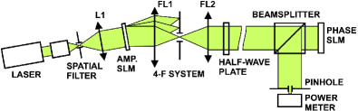
Figure 2: Experimental setup for the generation of beams with a von Mises distribution and subsequent detection of the associated angular-momentum components.

When the field impinging on the phase SLM has a structure $\sum_{n=-\infty}^{\infty}a_{n}\exp(in\phi)$, the hologram modifies its helicity so that the reflected beam can be written as $\sum_{n=-\infty}^{\infty}a_{n}\exp[i(n+m)\phi]$. The components for which $n+m=0$ present no helicity and their intensity profile consists of a light spot localized at the center of the beam. The other components have a nonzero helicity and the center of the intensity pattern remains dark. From this fact, the weight coefficients of the superposition can be determined by selective intensity measurements performed by a pinhole and a power meter.

A Laguerre-Gauss beam was used to align the setup and subsequently a beam with a von Mises distribution (18) of the transversal amplitude was generated. Each angular amplitude width was scanned for values of the helicities from $n=-20$ to $n=20$. Experimentally measured uncertainty products are depicted in Fig. 1 by solid circles.

Given the accuracy of the measurements (indicated by error bars in Fig. 1), they fit quite well the theoretical predictions. Our present experiment distinguishes between the uncertainty product of optimal states and the ideal limit. It is, however, not possible to dicriminate between the Mathieu and von Mises beams. Keeping in mind that von Mises and Mathieu states play the same role for the spatial degrees of freedom as Gaussian states for quadratures, the observation of the nonclassical behavior of angle and angular momentum is a challenging problem left for future studies.

In conclusion, we have formulated the uncertainty relations for angle and angular momentum based on dispersion as a correct statistical measure of error. The optimal states were derived and identified with the Mathieu wave functions. An optical test of the derived uncertainty relations was proposed and performed experimentally.

We acknowledge discussions with Hubert de Guise. This work was supported by the Czech Ministry of Education, Project MSM6198959213, the Czech Grant Agency, Grant 202/06/307, and the Spanish Research Directorate, Grant FIS2005-06714.

References

- (1) L. Allen, S. M. Barnett, and M. J. Padgett, Optical Angular Momentum (Institute of Physics, Bristol, 2003).
- (2) L. Allen, M. W. Beijersbergen, R. J. C. Spreeuw, and J. P. Woerdman, Phys. Rev. A 45, 8185 (1992).
- (3) S. J. van Enk and G. Nienhuis, Opt. Commun. 94, 147 (1992).
- (4) A. Wünsche, J. Opt. B: Quantum Semiclassical Opt. 6 S47 (2004).
- (5) G. F. Calvo, A. Picón, and E. Bagan, Phys. Rev. A 73, 013805 (2006).
- (6) N. B. Simpson, K. Dholakia, L. Allen and M. J. Padgett, Opt. Lett. 22, 52 (1997).
- (7) P. Galajda and P. Ormos, Appl. Phys. Lett. 78, 249 (2001).
- (8) L. Paterson, M. P. McDonald, J. Arlt, W. Sibbett, P. E. Bryant, and K. Dholakia, Science 292, 912 (2001).
- (9) A. Mair, A. Vaziri, G. Weihs, and A. Zeilinger, Nature (London) 412, 313 (2001).
- (10) G. Molina-Terriza, J. P. Torres, and L. Torner, Phys. Rev. Lett. 88, 013601 (2002).
- (11) A. Vaziri, J. W. Pan, T. Jennewein, G. Weihs, and A. Zeilinger, Phys. Rev. Lett. 91, 227902 (2003).
- (12) G. Molina-Terriza, A. Vaziri, J. Řeháček, Z. Hradil, and A. Zeilinger, Phys. Rev. Lett. 92, 167903 (2004).
- (13) A. Aiello, S. S. R. Oemrawsingh, E. R. Eliel, and J. P. Woerdman, Phys. Rev. A 72, 052114 (2005).
- (14) S. Franke-Arnold, S. M. Barnett, E. Yao, J. Leach, J. Courtial, and M. Padgett, New J. Phys. 6, 103 (2004).
- (15) D. T. Pegg, S. M. Barnett, R. Zambrini, S. Franke-Arnold, and M. Padgett, New J. Phys. 7, 62 (2005).
- (16) J. Leach, M. J. Padgett, S. M. Barnett, S. Franke-Arnold, and J. Courtial, Phys. Rev. Lett. 88, 257901 (2002).
- (17) V. Peřinova, A. Lukš, and J. Peřina, Phase in Optics (World Scientic 1998, Singapore).
- (18) A. Luis and L. L. Sánchez-Soto, Prog. Opt. 44, 421 (2000).
- (19) A. Luis and L. L. Sánchez-Soto, E. Phys. J. D 3, 195 (1998).
- (20) C. R. Rao, Linear Statistical Inference and its Applications (Wiley, New York, 1965).
- (21) L. C. Biedenharn and J. D. Louck, Angular Momentum in Quantum Physics: Theory and Application (Addison-Wesley, Massachusetts, 1981).
- (22) N. W. McLachlan, Theory and Application of Mathieu Functions (Oxford University Press, New York, 1947).
- (23) D. Frenkel and R. Portugal, J. Phys. A 34, 3541 (2001).
- (24) N. I. Fisher, Statistical Analysis of Circular Data (Cambridge University Press, Cambridge, 1995).
- (25) E. Breitenberger, Found. Phys. 15, 353 (1985).
- (26) U. Lund and S. Rao Jammalamadaka, J. Stat. Comput. Sim. 67, 319 (2000).