Efficient Generation of Generic Entanglement

Abstract

We find that generic entanglement is physical, in the sense that it can be generated in polynomial time from two-qubit gates picked at random. We prove as the main result that such a process generates the average entanglement of the uniform (unitarily invariant) measure in at most $O(N^{3})$ steps for $N$ qubits. This is despite an exponentially growing number of such gates being necessary for generating that measure fully on the state space. Numerics furthermore show a variation cut-off allowing one to associate a specific time with the achievement of the uniform measure entanglement distribution. Various extensions of this work are discussed. The results are relevant to entanglement theory and to protocols that assume generic entanglement can be achieved efficiently.

Introduction — Entanglement has traditionally been viewed as a fundamental tool for studies of the foundations of quantum mechanicsgenovese . More recently, the viewpoint of using entanglement as a resource has also gained prominence; see Plenio V 05 for a recent review. While a great deal of insight into the structure of two-particle entanglement has been gained, it has become equally clear that the complexity and diversity of multi-particle entanglement grows exponentially with the number of particles. It is thus difficult to imagine a structurally simple theory that characterizes and quantifies all details of multi-particle entangled states. On the other hand one may expect that large numbers of particles admit a notion of typical entanglement properties for which a structurally simple theory may be developed. This intuition gives hope that significant progress can be made by restricting attention to entanglement properties that are typical (generic) relative to the uniform (unitarily invariant) measure, the unbiased distribution of pure states. In this setting it was demonstrated that typically pure states of large numbers of spins exhibit maximal bi-partite pageandfoong ; lubkin ; lloyd ; hayden and multi-partite entanglement hayden . This suggests that the exploration of the entanglement properties of generic states is a promising approach.
But a big question mark exists as to whether statements about generic states relative to the uniform measure are physically relevant. This is because the generation of a typical unitary requires a sequence of 2-qubit unitaries whose length grows exponentially in the number of qubits NC , even if one allows for a finite fixed fidelity. Thus achieving the uniform distribution to a fixed accuracy requires sequences of random 2-qubit unitaries that grow exponentially with the size of the system, and quickly becomes unphysical, see e.g. emerson1 ; emerson2 ; emerson3 ; smith . One could then argue that the entanglement properties of generic quantum states are mathematically sound and interesting but physically irrelevant, as a system undergoing a randomisation of its state through two-party interactions would only get close to the uniform measure in an unfeasibly long time. On the other hand, entanglement properties represent a restricted class of physical properties of a quantum state. Accordingly the faithful reproduction of generic entanglement properties may be possible with far fewer physical resources, i.e. 2-qubit gates, than those required for the generation of the expectation value for an arbitrary observable.

It is thus crucial to explore whether generic entanglement properties can be obtained efficiently, i.e. polynomially in the number of qubits, using only one- and two-qubit gates. The present work answers this question positively (c.f. Figure 1).

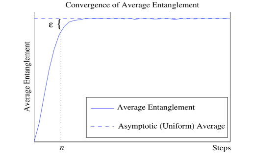
Figure 1: Typical numerical simulation using the random circuit. The entanglement average of the uniform measure is reached to an accuracy $\varepsilon$ in $n$ steps. We prove that it suffices with $n=O(N^{3})$ to achieve a fixed $arbitrary$ $\varepsilon$ accuracy when increasing $N$.

Our results support the physical relevance of the exploration of generic entanglement towards a structurally simple entanglement theory and have direct practical relevance since certain quantum information processing protocols such as abeyesinghe ; harrow ; hayden ; buhrman assume that generic entanglement can be generated efficiently.

The presentation proceeds as follows. We firstly define the key process that is used throughout this work: random two qubit interactions, modeled as random circuits on a quantum computer. Then we prove that the generic entanglement average as well as the purity of a subsystem are achieved efficiently and that the so generated states are typically very close to maximally entangled. This is followed by numerical evidence that the achievement of generic entanglement can be associated with a specific time, the variation cut-off, for large systems. We finish with a discussion and conclusion.

The setting – We consider a set of $N$-qubits split into two subsets $A$ (with $N_{A}$ qubits) and $B$ (with $N_{B}$ qubits). Let $|\,\psi_{0}\rangle$ be a initial state in $AB$ and consider a random circuit $C_{n}$ consisting of $n$ randomly chosen two-qubit quantum gates. Define $|\,\psi_{n}\rangle=C_{n}|\,\psi_{0}\rangle$ and the reduced density matrix $\rho_{A,n}=Tr_{B}(|\,\psi_{n}\rangle\langle\psi_{n}\,|)$ of system A. Then the entanglement in the state is given by $E(\psi_{n})=S(\rho_{A,n})$ and its purity by $Tr(\rho_{A,n}^{2})$.

Definition of the random circuit – The random circuit $C_{n}$ is a product $W_{n}\ldots W_{1}$ of two-qubit gates where each $W_{i}$ is independently chosen in the following way: A pair of distinct integers $c\neq t$ is chosen uniformly at random from $\{1,\dots,N\}$. Next, single-qubit unitaries $U[c]$ and $V[t]$ acting on qubit $c$ and $t$ respectively are drawn independently from the uniform measure on $U(2)$. Then $W=CNOT[c,t]U[c]V[t]$ where $CNOT[c,t]$ is the controlled-NOT gate with control $c$ and target $t$ gates .

Asymptotics of random circuit — The circuit, acting on $N$ qubits, will asymptotically induce the uniform measure on states (see e.g. emerson2 ). In the above setting for states distributed according to the uniform measure the average bipartite entanglement can be found exactly pageandfoong and is bounded from below such that $\mathbb{E}\left[E(\psi_{n})\right]\geq N_{A}-\frac{1}{\ln 2}2^{-t}$ where $N_{B}-N_{A}=t\geq 0$ hayden . Likewise we find that the average purity of the subsystem $A$ is given by $(2^{N_{A}}+2^{N_{B}})/(2^{N}+1)$ consistent with smith . Furthermore, the distributions for entanglement and purity concentrate around their average with increasing $N$ lubkin ; lloyd ; pageandfoong ; hayden . Thus one is overwhelmingly likely to find near-maximal entanglement for large systems.

Main Theorem — We will now be concerned with the approach to the asymptotic regime. For the above setting we prove that, independently of the initial state $|\psi_{0}\rangle$, convergence of the expected entanglement to its asymptotic value to an arbitrary fixed accuracy $\varepsilon$ is achieved after a number of random two-qubit gates that is polynomial in the number of qubits. More precisely we find:

Theorem 1

Suppose that $N_{B}-N_{A}=t\geq 0$ and that some arbitrary $\varepsilon\in(0,1)$ is given. Then for a number $n$ of gates in $C_{n}$ satisfying

$$\vspace{-0.4cm}n\geq 9N(N-1)[(3\ln 2)N+\ln\varepsilon^{-1}]/4,$$

$$\mbox{we have}\;\;\;\;\;\;\;\;\;\;\;\;\mathbb{E}\left[E(\psi_{n})\right]\geq N_{A}-(2^{-t}+\varepsilon)/\ln 2.$$ (1)

$$\mbox{and }\;\;\;\;\;\;\mathbb{E}[\max_{|\Psi\rangle_{AB}=maxent}|\langle\psi_{n}|\Psi\rangle|]\geq 1-\sqrt{\frac{2^{-t}+\epsilon}{2\ln 2}}.$$ (2)

Eq. (2), follows from eq. (1) employing $\sqrt{2S(\sigma\|\rho)}\geq tr|\sigma-\rho|_{1}$, where $S$ is the relative entropy, and $\frac{1}{2}tr|\sigma-\rho|_{1}\geq 1-tr\sqrt{\sqrt{\rho}\sigma\sqrt{\rho}}$ as well as Uhlmann’s TheoremNC . To prove eq. (1) we prove a Lemma that considers the quantity $\mathbb{E}\left[Tr(\rho_{A,n}^{2})\right]$.

Lemma 1

For arbitrary $N,N_{A},N_{B}$ and all $n$ we have

$$\vspace{-0.2cm}\left|\mathbb{E}\left[Tr(\rho_{A,n}^{2})\right]-\frac{2^{N_{A}}+2^{N_{B}}}{2^{N}+1}\right|\leq 4^{N}e^{-\frac{4n}{9N(N-1)}}.\vspace{-0.1cm}$$

To see that Lemma 1 implies Theorem 1 note first that $E(\psi_{n})=S(\rho_{A,n})\geq-\log_{2}Tr(\rho_{A,n}^{2})$. By convexity we then find $\mathbb{E}\left[-\log_{2}Tr(\rho_{A,n}^{2})\right]\geq-\log_{2}(\mathbb{E}\left[Tr(\rho_{A,n}^{2})\right])$ and a direct computation using $\ln(1+x)\leq x$ for $x\geq 0$ completes the argument.

Proof of Lemma 1 – We proceed to outline the proof of Lemma 1 below, omitting some tedious but straightforward calculations to improve clarity. We begin with a useful representation of quantum states in terms of Pauli-operators. Indeed, $|\,\psi_{n}\rangle\langle\psi_{n}\,|=\sum_{p\in\{0,x,y,z\}^{N}}\xi_{n}(p)2^{-N/2}\otimes_{i=1}^{N}\sigma^{p_{i}}[i]$, where each $\xi_{n}(p)=2^{-N/2}Tr(\otimes_{i=1}^{N}\sigma^{p_{i}}[i]|\,\psi_{n}\rangle\langle\psi_{n}\,|)$ and $\sigma^{p_{i}}[i]$ is a Pauli operator acting on qubit $i$ gates . Then for the reduced density operator $\rho_{A,n}=Tr_{B}(|\,\psi_{n}\rangle\langle\psi_{n}\,|)$ we find

$$\mathbb{E}\left[Tr(\rho^{2}_{A,n})\right]=2^{N_{B}}\sum\limits_{\{p\,:\,\forall i\not\in A,\;p_{i}=0\}}\mathbb{E}\left[\xi_{n}^{2}(p)\right].$$ (3)

The main purpose will now be to analyze the evolution of the expected values of the squared coefficients, $\mathbb{E}\left[\xi_{n}^{2}(p)\right]$

Evolution of the coefficients – The key idea of the proof relies on the observation that the $\mathbb{E}\left[\xi_{n}^{2}(p)\right]$ form a probability distribution on $\{0,x,y,z\}^{N}$ for all $n$ and that these probabilities evolve as a Markov chain with transition matrix $P$ which takes $q$ distributed according to $(\mathbb{E}\left[\xi_{n}^{2}(q)\right])_{q}$ in one step to $p$ distributed according to $(\mathbb{E}\left[\xi_{n+1}^{2}(p)\right])_{p}$. To determine $P$ we consider the action of a random unitary $W_{n}$ at time $n$ that acts on qubits $c,t$ in state $|\psi_{n}\rangle$. This results in $\mathbb{E}\left[\xi_{n+1}^{2}(p)\!\mid\!\psi_{n},c,t\right]\!=\!1/16\!\!\!\!\!\!\!\!\!\sum\limits_{q,q^{\prime}\in\{0,x,y,z\}^{N}\!:\!\forall i\not\in\{c,t\},\,q_{i}\neq q^{\prime}_{i}}\!\!\!\!\!\!\!\!\!\!\!\!\!\!\!\!\xi_{n}(q)\xi_{n}(q^{\prime})\!\times\times\mathbb{E}\left[Tr[U\sigma^{q_{c}}[c]U^{\dagger}\sigma^{\hat{p}_{c}}[c]]Tr[U\sigma^{q^{\prime}_{c}}[c]U^{\dagger}\sigma^{\hat{p}_{c}}[c]]\right]\times\times\mathbb{E}\left[Tr[V\sigma^{q_{t}}[t]V^{\dagger}\sigma^{\hat{p}_{t}}[t]]Tr[V\sigma^{q^{\prime}_{t}}[t]V^{\dagger}\sigma^{\hat{p}_{t}}[t]]\right]$ , where the $(\hat{p}_{c},\hat{p}_{t})$ are uniquely determined by $CNOT[c,t]\sigma^{p_{c}}[c]\sigma^{p_{t}}[t]CNOT[c,t]\!\!=\!\!\pm\sigma^{\hat{p_{c}}}[c]\sigma^{\hat{p_{t}}}[t]$. Direct calculation with the uniform measure on $U(2)$ shows that the products of expectations in the sum vanish unless $q=q^{\prime}$. Then with the Kronecker symbol $\delta_{i,j}$ we find $\mathbb{E}\left[\xi_{n+1}^{2}(p)\mid\psi_{n},c,t\right]=\!\!\!\sum\limits_{q\in\{0,x,y,z\}^{N}}\!\!\!\!\!\!\!\!P^{(c,t)}(q,p)\!\!\!\prod\limits_{i\not\in\{c,t\}}\!\!\delta_{q_{i},p_{i}}\xi^{2}_{n}(q)$ where $P^{(c,t)}(q,p)\!\!=\!\!1$ if $\hat{p}_{c}\!\!=\!\!\hat{p}_{t}\!\!=\!\!q_{c}\!\!=\!\!q_{t}\!\!=\!\!0$; $P^{(c,t)}(q,p)\!\!=\!\!1/3$ if $\hat{p}_{c}\!\!=\!\!q_{c}\!\!=\!\!0$ and $\hat{p}_{t}\!,\!q_{t}\!\!\neq\!\!0$ or if $\hat{p}_{t}\!\!=\!\!q_{t}\!=\!0$ and $\hat{p}_{c}\!,\!q_{c}\!\!\!\neq\!\!\!0$; and $P^{(c,t)}(q,p)\!\!=\!\!1/9$ otherwise. Averaging $P^{(c,t)}(q,p)\prod_{i\not\in\{c,t\}}\delta_{q_{i},p_{i}}$ over the $N(N\!-\!1)$ choices of $c,t$ produces the entry $P(q,p)$ of the transition matrix of the desired Markov chain for $(\mathbb{E}\left[\xi_{n}^{2}(q)\right])_{q}$.

Simplifying the Markov chain – Our aim is the evaluation of eq. (3) and it turns out that this can be done via a simplified Markov Chain. Consider $\{q(n)=(q(n)_{1}q(n)_{2}\dots q(n)_{N})\}_{n\geq 1}$ as an $n$-step evolution of our Markov chain $P$. Then the sets $S(n)=\{i\in\{1,\dots,N\}\,:\,q(n)_{i}\neq 0\}$, identifying the nonzero elements of $q(n)$ also form a Markov Chain. Using $S(n)$ in eq. (3) we find

$$\mathbb{E}\left[Tr(\rho^{2}_{A,n})\right]=2^{N_{B}}\mathbb{P}\left(S(n)\subset A\right).$$ (4)

Thus we need only to consider the chain $\{S(n)\}_{n}$.

Convergence rate of the Markov chain. – As it turns out, our chain is almost ergodic: removing the isolated state $S(n)=\emptyset$, we obtain an ergodic chain on $\Omega=2^{\{1,\dots,N\}}\backslash\{\emptyset\}$. Since $\mathbb{P}\left(S(n)=\emptyset\right)=\mathbb{P}\left(S(0)=\emptyset\right)=2^{-N}$, determining the convergence rate to the equilibrium of $S(n)$ on $\Omega$ given by ${\cal M}(S)=3^{|S|}/(4^{N}-1)$, $S\in\Omega$ is sufficient for our purposes. Let $Q=(Q(S,S^{\prime}))_{S,S^{\prime}\in\Omega}$ be the transition matrix of the restricted $S(n)$ chain. It has largest eigenvalue $1$ whose eigenvector determines the steady state solution ${\cal M}$. The difference to the second largest eigenvalue, the spectral gap $\lambda_{Q}$, bounds the convergence rate to the steady state: for any initial distribution vector $v$, the component of $Q^{n}v$ orthogonal to ${\cal M}$ shrinks exponentially fast with $\lambda_{Q}n$. A quantitative result is provided in Chapter 2 of montenegro (see Corollary 2.15): since our $Q$ is a reversible chain with $Q(S,S)\geq 1/2$ for all $S\in\Omega$, we obtain $|\mathbb{P}\left(S(n)\!\!\subset A\right)\!\!\!-\!\!\!\sum_{\emptyset\neq S\subset A}\!\!{\cal M}(S)|\leq\!\!e^{-\lambda_{Q}n}/\sqrt{\min_{T}{\cal M}(T)}\!\!\leq\!\!2^{N}e^{-\lambda_{Q}n}.$ We have $\sum_{\emptyset\neq S\subset A}{\cal M}(S)\!\!=\!\!(4^{N_{A}}-1)/(4^{N}-1)$. Putting back the isolated state $\emptyset$ into the calculations, applying (4) and noting that $2^{N_{B}}\leq 2^{N}$ yields $\left|\mathbb{E}\left[Tr(\rho^{2}_{A,n})\right]-\frac{2^{N_{A}}+2^{N_{B}}}{2^{N}+1}\right|\leq 4^{N}e^{-\lambda_{Q}n}.$ All that remains is to show that $\lambda_{Q}\geq 4/9N(N-1)$. We use a well-known variational principle for $\lambda_{Q}$footnote2 :

$$\lambda_{Q}=\inf\frac{\sum_{S,S^{\prime}\in\Omega}{\cal M}(S)Q(S,S^{\prime})(f(S)-f(S^{\prime}))^{2}}{\sum_{T,T^{\prime}\in\Omega}{\cal M}(T){\cal M}(T^{\prime})(f(T)-f(T^{\prime}))^{2}},$$ (5)

where the $\inf$ is taken over non-constant $f:\Omega\to\mathbb{R}$. This is an application of Raleigh’s principle to the second smallest eigenvalue of $I-Q$, which is precisely $\lambda_{Q}$. Eq. (5) implies that if $R$ is the transition matrix of a Markov chain on $\Omega$ with same stationary distribution ${\cal M}$ and $\alpha R(S,S^{\prime})\leq Q(S,S^{\prime})$ for all $S,S^{\prime}\in\Omega$, then the gap $\lambda_{R}$ of $R$ satisfies $\lambda_{Q}\geq\alpha\lambda_{R}$. This allows us to estimate $\lambda_{Q}$ by comparison with a simpler chain diaconisSC . Indeed, our $R$ will be transition matrix of chain $\{B(n)\}$ on $\Omega$ defined as follows: Assume $B(n)=B$ and choose a $1\leq j\leq N$ uniformly at random. If $j\in B$ and $|B|\geq 2$, set $B(n+1)=B\backslash\{j\}$ with probability $1/3$ and $B_{n+1}=B$ with probability $2/3$. If $j\in B$ and $|B|=1$, do nothing. If $j\not\in B$, set $B(n+1)=B\cup\{j\}$. This is a biased random walk on the hypercube $2^{\{1,\dots,N\}}$ where transitions to state $\emptyset$ are suppressed. A coupling argument following e.g. Chapter 4 of levinPW shows that $R$ has a spectral gap $\geq 1/3N$. Moreover, one can check that $\alpha R(S,S^{\prime})\leq Q(S,S^{\prime})$ with $\alpha=4/3(N-1)$. It follows that $\lambda_{Q}\geq\alpha\lambda_{R}\geq 4/9N(N-1)$, as desired, and the proof is finished. Numerics indicate convergence in approximately $N\log N$ steps, so our bound is not tight.

Observe cut-off – Many Markov chains exhibit the so called ”cut-off effect”diaconis . The cut-off refers to an abrupt approach to the stationary distribution occurring at a certain number of steps taken in the chain. Say we have a Markov chain defined by its transition matrix P, and that it converges to a stationary distribution $\pi$. Initially the total variation distance $TV=\parallel P-\pi\parallel=sup\mid P(E)-\pi(E)\mid$ between the corresponding probability distributions is given by $TV=1$. After $k$ steps this distance is given by $TV(k)=\parallel P^{k}-\pi\parallel$. A cut-off occurs, basically, if $TV(k)\simeq 1$ for $k=0,1,2,...a$ and therafter falls quickly such that after a few steps $TV(k)\simeq 0$. As we increase the size of the state space, the ratio of the number of steps during which the abrupt approach takes place and $a$ should vanish asymptotically. Then we can say that the randomisation occurs at $a$ steps. Rigorously, this may be stated as follows diaconis . Let $P_{n}$, $\pi_{n}$ be Markov Chains on sets $\chi_{n}$. Let $a_{n}$, $b_{n}$ be functions tending to infinity, with ${b_{n}}/{a_{n}}$ tending to zero. Say the chains satisfy an $a_{n}$, $b_{n}$ cutoff if for some starting states $x_{n}$ and all fixed real $\theta$ with $k_{n}=\lfloor a_{n}+\theta b_{n}\rfloor$, then $\parallel P_{n}^{k_{n}}-\pi_{n}\parallel\longrightarrow c(\theta)$ with $c(\theta)$ a function tending to zero for $\theta$ tending to infinity and to 1 for $\theta$ tending to minus infinity. Here we observe this behaviour in the entanglement distribution, a functional of the Markov chain on unitaries given by the random circuit, and we accordingly term this a cut-off.

Numerical Observation​​ – Numerical simulations indicate a cut-off effect in the entanglement probability distribution under the random circuit on $|\,0\rangle^{\otimes N}$ may be observed both for single qubit gates drawn from the uniform measure on U(2) and for stabilizer gates; see Figure 2.

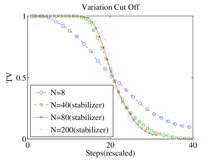
Figure 2: Observe a variation Cut-Off of the entanglement probability distribution compared with that of the uniform measure as determined numerically. The state space has been discretised by rounding off entanglement values to the nearest integer. We observe that $TV\simeq 1$ for a while and then falls. Finally there is a stage where $TV\simeq 0$. The effect becomes more pronounced with increasing $N$. The results for $N>8$ are done using the stabilizer random circuit.

The simulations using stabilizer gates allow us to consider far larger systems sizes. Here we choose the single qubit gates $U$ and $V$ from the set $\{\sigma^{x},\sigma^{y},\sigma^{z},S,H\}$ gates with equal probability. It should be noted that the proof of Lemma 1 still holds (see longer for details) and the entanglement behaviour will remain similar . The restriction allows us to use the efficient stabilizer formalism gottesman2 and the tools developed in audenaert which in turn allows for an efficient evaluation of state properties.

Extensions of the present result – Similar methods can be used to address the mixed state setting through tracing out part of the system on which the random circuit is applied. Multipartite entanglement measures based on average purities Plenio V 05 can be considered with the results established here. We also anticipate that one can use similar techniques to obtain rigorous statements about the convergence rates of finite temperature Markov Process Quantum Monte Carlo simulations.

Our results may be applied to the protocols for superdense coding of quantum states presented in abeyesinghe ; harrow ; hayden to replace the inefficient process of creating random unitaries distributed according to the Haar measure by our efficient random circuits. After that replacement, Theorem 1 may be applied directly to verify that the main Lemma 1 of harrow still holds. It is an open question whether the performance of the protocols in abeyesinghe ; hayden ; buhrman is adversely affected by this substitution. This cannot be decided on the basis of Theorem 1 alone but we expect that similar techniques as described here and in longer will be able to decide this. The results of this work as well as the above extensions will be presented in detail in forthcoming publications.

Conclusion — In this work we have proved that the average entanglement over the unitarily invariant measure is reached in a time that is polynomial in the size of the system by a quantum random process that is restricted to random two-qubit interactions. We also provided numerical evidence that for large systems the entanglement distribution of the uniform measure is achieved at a specific point in time, the variation cut-off. Our results demonstrate that the entanglement properties of generic entanglement are physical in the sense that they can be generated efficiently from random sequences of two-qubit gates. We have described extensions, including how this knowledge can be applied to render certain protocols efficient.

Acknowledgements — We gratefully acknowledge early discussions with J. Oppenheim and discussions with T. Rudolph, G. Smith, and J. Smolin. M. B. P. was funded by the EPSRC QIPIRC, The Leverhulme Trust, EU Integrated Project QAP, and the Royal Society; O. D. by the Institute for Mathematical Sciences of Imperial College, and R. O. by NSA and ARDA through ARO Contract No. W911NF-04-C-0098.

References

- (1) M. Genovese, Phys. Rep. 413, 319 (2005).
- (2) M.B. Plenio and S. Virmani, Quant. Inf. Comp. 7, 1 (2006).
- (3) P. Hayden, D.W. Leung and A. Winter, Comm. Math. Phys. 265, 95 (2006) .
- (4) E.Lubkin, J. Math. Phys 19, 1028 (1978).
- (5) S.Lloyd and H.Pagels, Ann. of Phys. 188, 186 (1988).
- (6) D.N.Page, Phys. Rev. Lett. 71, 1291 (1993). S.K Foong and S.Kanno, Phys. Rev. Lett. 72, 1148 (1994).
- (7) M.A. Nielsen and I. Chuang, Quantum Information and Computation, Cambridge Univ. Press.
- (8) J. Emerson, E. Livine and S. Lloyd, Phys. Rev. A. 72, 060302 (2005).
- (9) J. Emerson, Y.S. Weinstein, M. Saraceno, S. Lloyd and D.G. Cory, Science 302, 2098 (2003).
- (10) G.Smith and D.W.Leung, Phys. Rev. A 74, 062314 (2006).
- (11) J. Emerson, QCMC04, AIP Conf. Proc. 734, 139 (2004).
- (12) A.Abeyesinghe, P.Hayden, G.Smith and A. Winter, IEEE TIT 52, 8, 3635 (2005).
- (13) H. Buhrman, M. Christandl, P. Hayden, H.K. Lo, and S. Wehner, arXiv:quant-ph/0504078.
- (14) A. Harrow, P. Hayden, and D. Leung, Phys. Rev. Lett., 92, 187901 (2004).
- (15) J. Emerson, R. Alicki and K. Zyczkowski, J. Opt. B 7, 1347 (2005).
- (16) D.P. DiVincenzo, D.W. Leung, and B.M. Terhal, IEEE Trans. Inf. Theory, 48(3), 580 (2002).
- (17) D. Gottesman, arXiv:quant-ph/9807006.
- (18) K.M.R. Audenaert and M.B. Plenio, New J. Phys. 7, 170 (2005). Computer codes downloadable at www.imperial.ac.uk/quantuminformation.
- (19) O.C.O.Dahlsten and M.B.Plenio, Quant. Inf. Comp. 6, 527, (2006).
- (20) P.Diaconis, Proc. Natl. Acad. Sci. USA 93, 1659, (1996).
- (21) In the computational basis: .
- (22) Markov Chains and Mixing Times D. A. Levin, Y. Peres and E. L. Wilmer, book draft at http://www.oberlin.edu/markov/
- (23) P. Diaconis; L. Saloff-Coste Ann. of Appl. Prob., 3, No. 3., p.696, (1993).
- (24) R. Montenegro and P. Tetali, Ser. Found., Trends, Th. Comp. Sci., 1:3, NOW Publ., Boston-Delft, (2006).
- (25) See Lemma 2.21 in montenegro . Our numerator is twice their Dirichlet form (Defn. 2.1) and our denominator is twice the variance.
- (26) J. Calsamiglia, L. Hartmann, W. Dür, and H.-J. Briegel, Phys. Rev. Lett. 95, 180502 (2005).
- (27) O.C.O Dahlsten, R.Oliveira, M.B.Plenio, arXiv:quant-ph/0701125.