Preparation of a Single Photon in Time-bin Entangled States via Photon Parametric Interaction

Abstract

A novel method for preparation of a single photon in temporally-delocalized entangled modes is proposed and analyzed. We show that two single-photon pulses propagating in a driven nonabsorbing medium with different group velocities are temporally split under parametric interaction into well-separated pulses. In consequence, the single-photon ”time-bin-entangled” states are generated with a programmable entanglement easily controlled by driving field intensity. The experimental study of nonclassical features and nonlocality of generated states by means of balanced homodyne tomography is discussed.

Entanglement and nonlocal correlations, besides their fundamental importance in the modern interpretation of quantum phenomena ein ; bell , are the basic concepts for realization of quantum information procedures ben . The entanglement between matter and light states is an essential element of quantum repeaters breig , the intermediate memory nodes in quantum communication network aimed at preventing the photon attenuation over long distances. The two-photon entanglement is a crucial ingredient for quantum cryptography ekert ; tittel , quantum teleportation bouw ; furus ; marc , and entanglement swapping zuk ; pan , which have been successfully realized during the last decade by utilizing two approaches, one based on continuous quadrature variables and the other using the polarization variables of quantized electromagnetic field braun . An essential step has been recently made in this direction by implementing robust sources producing the pairs of photons which are entangled in well-separated temporal modes (time-bins) brend . It has been shown brend ; ried that this type of entanglement, in contrast to other ones, can be transferred over significant large distances without appreciable losses that makes it much preferable for long-distance applications. From the fundamental viewpoint, of special interest is a single photon delocalized into two distinct spatial knill or temporal modes, for which case the nonlocality of quantum correlations is directly evident from the violation of Bell’s inequality formulated for the two-mode Wigner function bonas . This was verified experimentally by performing the homodyne detection of delocalized single-photon Fock states and reconstructing the corresponding Wigner function from homodyne data lvov ; babi ; zava . To date two approaches have been developed for preparation of a single-photon in two distinct temporal modes. In first one a time-bin qubit is created with the help of linear optics by passing a short pulse through Mach-Zehnder interferometer with different-length arms brend . The second approach is based on conditional measurement on quantum system of entangled signal-idler pairs generated via spontaneous parametric down conversion (SPDC) of successive pump pulses in a nonlinear crystal, when a detection of one idler photon tightly projects the signal field into a single-photon state coherently delocalized over two temporal modes zava .

In this paper we demonstrate a novel method for dynamical preparation of time-bin qubit. The basic idea is to create a parametric interaction between two single-photon pulses, which propagate in a driven medium without absorption and with slow, but different group velocities. Then, due to the cyclic parametric conversion of the fields and the group delay, each pulse experiences a temporal splitting into well-separated subpulses. Moreover, since the process is completely coherent, at the output of the medium the time-delocalized single-photon states are formed. A remarkable feature of our scheme is the ability to produce two and more output temporally-entangled modes. Another important advantage is a generation in a simple manner any desired entanglement by controlling the driving field intensity.

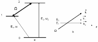
Figure 1: (a) Level scheme of atoms interacting with quantum fields $E_{1,2}$ and classical rf driving field of Rabi frequency $\Omega.$ (b) Geometry of fields propagation.

We consider an ensemble of $\Delta$-type cold atoms with level configuration as in Fig.1. Two quantum fields

$$E_{1,2}^{(+)}(z,t)=\sqrt{\frac{\hbar\omega_{i}}{2{\varepsilon}_{0}V}}\hat{\mathcal{E}}_{1,2}(z,t)\exp[i(k_{1,2}z-\omega_{1,2}t)]$$

co-propagate along the $z$ axis and interact with the atoms on the transitions $\mid 0$ $\rangle\rightarrow\mid 1$ $\rangle$  and $\mid 0$ $\rangle\rightarrow\mid 2$ $\rangle,$ respectively, while the electric-dipole forbidden transition $\mid 1$ $\rangle\rightarrow\mid 2$ $\rangle$ is driven by a classical and constant radio-frequency field (rf)with Rabi frequency $\Omega$ inducing a magnetic dipole or an electric quadruple transition between the two upper levels. Here the electric fields are expressed in terms of the operators $\hat{\mathcal{E}}_{i}(z,t)$ obeying the commutation relations

$$[\hat{\mathcal{E}}_{i}(z,t),\hat{\mathcal{E}}_{j}^{+}(z^{{}^{\prime}},t)]=L\delta_{ij}\delta(z-z^{{}^{\prime}})$$ (1)

where $L$ is the length of the medium. We describe the latter using atomic operators $\hat{\sigma}_{\alpha\beta}(z,t)$ $=\frac{1}{N_{z}}\underset{i=1}{\overset{N_{z}}{\sum}}\mid\alpha$ $\rangle_{i}\langle\beta\mid$ averaged over the volume containing many atoms $N_{z}=\frac{N}{L}dz\gg 1$ around position $z$, where $N$ is the total number of the atoms. In the rotating wave picture the interaction Hamiltonian is given by

$$H=-\hbar\frac{N}{L}\int\limits_{0}^{L}dz[g_{1}\hat{\mathcal{E}}_{1}\hat{\sigma}_{10}e^{ik_{1}z}+g_{2}\hat{\mathcal{E}}_{2}\hat{\sigma}_{20}e^{ik_{2}z}+\Omega\hat{\sigma}_{21}e^{ik_{\parallel}z}$$

$$+h.c.]$$ (2)

Here $k_{\parallel}=\vec{k}_{d}\hat{e}_{z}$  is the projection of the wave-vector of the driving field on the $z$ axis, $g_{\alpha}=\mu_{\alpha o}\sqrt{\frac{\hbar\omega_{i}}{2{\varepsilon}_{0}V}}$ is the atom-field coupling constants with $\mu_{\alpha\beta}$ being the dipole matrix element on the transition $\mid\alpha$ $\rangle\rightarrow\mid\beta$ $\rangle$ , and $V$ is the quantization volume taken to be equal to interaction volume. For simplicity, we discuss the case of exactly resonant interaction with all fields and, therefore, put in Eq.(1) the frequency detunings equal to zero, neglecting so the Doppler broadening, which in a cold atomic sample is smaller than all relaxation rates. Then, using the slowly varying envelope approximation, the propagation equations for the quantum field operators take the form:

$$\left(\frac{\partial}{\partial z}+\frac{1}{c}\frac{\partial}{\partial t}\right)\hat{\mathcal{E}}_{1}(z,t)=ig_{1}\frac{N}{c}\hat{\sigma}_{01}e^{-ik_{1}z}+\hat{F}_{1}$$ (3)

$$\left(\frac{\partial}{\partial z}+\frac{1}{c}\frac{\partial}{\partial t}\right)\hat{\mathcal{E}}_{2}(z,t)=ig_{2}\frac{N}{c}\hat{\sigma}_{02}e^{-ik_{2}z}+\hat{F}_{2}$$ (4)

where $\hat{F}_{i}(z,t)$ are the commutator preserving Langevin operators, whose explicit form is not of interest here.

In the weak-field (single-photon) limit, the equation of atomic coherences $\hat{\rho}_{0i}=\hat{\sigma}_{0i}e^{-ik_{i}z},\ \ i=1,2~{}\ \ \$and$\ \ \ \ \ \hat{\rho}_{12}=\hat{\sigma}_{12}e^{-i(k_{2}-k_{1})z}\$ are treated perturbatively in $\hat{\mathcal{E}}_{1,2}$. In first order only $\hat{\sigma}_{00}\simeq 1$ is different from zero and for these equations we get:

$$\frac{\partial}{\partial t}\hat{\rho}_{01}=-\Gamma_{1}\hat{\rho}_{01}+ig_{1}\hat{\mathcal{E}}_{1}\hat{\sigma}_{00}+i\Omega^{\ast}\hat{\rho}_{02}e^{i\bigtriangleup kz}-ig_{2}\hat{\mathcal{E}}_{2}\hat{\rho}_{21}$$ (5)

$$\frac{\partial}{\partial t}\hat{\rho}_{02}=-\Gamma_{2}\hat{\rho}_{02}+ig_{2}\hat{\mathcal{E}}_{2}\hat{\sigma}_{00}+i\Omega^{\ast}\hat{\rho}_{01}e^{-i\bigtriangleup kz}-ig_{1}\hat{\mathcal{E}}_{1}\hat{\rho}_{12}$$ (6)

$$\frac{\partial}{\partial t}\hat{\rho}_{12}=-(\Gamma_{1}+\Gamma_{2})\hat{\rho}_{12}-ig_{1}\hat{\mathcal{E}}_{1}^{\ast}\hat{\rho}_{02}+ig_{2}\hat{\mathcal{E}}_{2}\hat{\rho}_{10}$$ (7)

Here $2\Gamma_{1,2}$ are the decay rates of the excited states $\mid 1$ $\rangle$ and $\mid 2$ $\rangle$ and $\Delta k=k_{2}-k_{1}-k_{\parallel}$ is the wave-vector mismatch.

Further, we assume that the phase-matching condition $\Delta k=0$ is fulfilled in the medium. Then, the solution to Eqs.(5-7) to the first order in $\hat{\mathcal{E}}_{1,2}$ is readily found to be

$$\hat{\rho}_{01}=-i\frac{\Gamma}{D}g_{1}\hat{\mathcal{E}}_{1}-i\frac{\Omega^{2}-\Gamma^{2}}{D^{2}}g_{1}\frac{\partial}{\partial t}\hat{\mathcal{E}}_{1}-\frac{\Omega}{D}g_{2}\hat{\mathcal{E}}_{2}+\frac{2\Gamma\Omega}{D^{2}}g_{2}\frac{\partial}{\partial t}\hat{\mathcal{E}}_{2},$$ (8)

$$\hat{\rho}_{02}=\hat{\rho}_{01}(1\leftrightarrow 2),\ \ \ \text{ }D=\Omega^{2}+\Gamma^{2}.$$ (9)

where, for simplicity, the optical decay rates are taken to be the same: $\Gamma_{1}=\Gamma_{2}=\Gamma$. The first terms in right hand side (RHS) of Eqs.(8,9) are responsible for linear absorption of quantum fields and define the field absorption coefficients $k_{i}=\frac{g_{i}^{2}\Gamma N}{c\Omega^{2}}$ upon substituting these expressions into Eqs.(3,4). Here the condition of electromagnetically induced transparency (EIT, refs.harris ; mfleis ) $\Omega\gg\Gamma_{1,2}$ is assumed to be satisfied for both transitions with weak-field coupling. The second terms in RHS of Eqs.(8,9) represent the dispersion contribution to the group velocities of the pulses, while the two rest terms describe the parametric interaction between the fields. We require the photon absorption to be strongly reduced by imposing the condition $k_{i}L\ll 1.$ Another limitation follows from $\Delta\omega_{EIT}T\geq 1$ indicating that the initial spectrum of quantum fields is contained within the EIT window $\Delta\omega_{EIT}=\frac{\Omega^{2}}{\Gamma}$ $\frac{1}{\sqrt{\alpha}}$ fleis , where $T$ is a duration of weak-field pulses, $\alpha=\mathcal{N}\sigma L$ is optical depth, $\sigma=\frac{3}{4\pi}\lambda^{2}$ is resonant absorption cross-section and $\mathcal{N}$ is the atomic number density. Finally, the length of the pulses has to fit the length of the medium: $Tv_{i}<L$ with $v_{i}=\frac{c\Omega^{2}}{g_{i}^{2}N}$ being the group velocity of the $i$-th field. Taking into account that $k_{i}L\sim\Gamma^{2}\alpha/\Omega^{2},$ this set of limitations yields

$$\frac{\Omega^{2}}{\Gamma^{2}}>>\alpha\text{ \ \ \ \ and \ }\frac{1}{\sqrt{\alpha}}\ll\frac{Tv_{i}}{{}_{L}}<1\text{\ \ \ }$$ (10)

It is worth noting that upon satisfying the conditions (10), the dominant contribution to the parametric coupling between the photons is the third term in RHS of Eq.(8,9), because in this case the last term becomes strongly suppressed by the factor $\Omega^{2}T/\Gamma>>1.$

It is useful at this point to consider numerical estimations. The sample is chosen to be ${}^{85}Rb$ vapor with the ground state $5S_{1/2}(F_{g}=3)$ and exited states $5P_{3/2}(F_{e}=2),$ $5P_{3/2}(F_{e}=3)$ of $Rb$ atom as the states $\mid 0$ $\rangle$ and $\mid 1$ $\rangle,\mid 2$ $\rangle$  in Fig.1 , respectively, using the following parameters: light wavelength $\lambda\simeq 0.8\mu$m, $\Gamma=2\pi\ast 3$ MHz, atomic density $\mathcal{N}\sim 10^{12}$cm^-3 in a trap  of length $L\sim 100$ $\mu$m, $\Omega\sim 10\Gamma,$ and the input pulse duration $T\simeq$ 2$\div$3ns. In this case $\alpha\simeq 16,$ $v_{2}\sim 10^{4}m/s$, $v_{1}\sim 0.3v_{2},$ and $k_{i}L\leqslant 0.2.$ All of the parameters we use in our calculations appear to be within experimental reach, including initial single-photon wave packets with a duration of several ns satisfying the narrow-line limitation discussed above. The standard method for producing single photons based on SPDC in nonlinear crystals does not fit our purpose due to too broad linewidth ($\sim 10$nm) of generated light. Recently, a source of narrow-bandwidth, frequency tunable single photons with properties allowing to excite the narrow atomic resonances has been created chou ; eis .

Then, taking into account that in the absence of photon losses the noise operators $\hat{F}_{i}$ in Eqs.(5) give no contribution, the simple propagation equations for the field operators are finally obtained:

$$\left(\frac{\partial}{\partial z}+\frac{1}{v_{1}}\frac{\partial}{\partial t}\right)\hat{\mathcal{E}}_{1}(z,t)=-i\beta\hat{\mathcal{E}}_{2}$$ (11)

$$\left(\frac{\partial}{\partial z}+\frac{1}{v_{2}}\frac{\partial}{\partial t}\right)\hat{\mathcal{E}}_{2}(z,t)=-i\beta\hat{\mathcal{E}}_{1}$$ (12)

where $\beta={g_{1}g_{2}N/c\Omega}$ is the parametric coupling constant. It is easy to check that these equations preserve the commutation relations (1). Note that for the parameters above, the parametric interaction between the photons is highly strong $\beta L\sim 3$.

The formal solution of Eqs.(11,12) for field operators in the region $0\leqslant z\leqslant L$ is written as

$$\hat{\mathcal{E}}_{i}(z,t)=\hat{\mathcal{E}}_{i}(0,\ t-z/v_{i})+\int\limits_{0}^{z}dx\{\hat{\mathcal{E}}_{i}(0,\ t-z/v_{i}-\frac{\Delta v_{ij}}{v_{i}v_{j}}(z-x))$$

$$\ast\frac{\partial J_{0}(\psi)}{\partial z}-i\beta\ \hat{\mathcal{E}}_{j}(0,\ t-z/v_{i}-\frac{\Delta v_{ij}}{v_{i}v_{j}}(z-x))\ J_{0}(\psi)\},\$$ (13)

where $i,j=1,2$  and $j\neq i.$ The Bessel function $\ J_{0}(\psi)$ depends on $z$ via $\psi=2\beta\sqrt{x(z-x)}$ , $\Delta v_{ij}=v_{i}-v_{j}$ is the difference of group velocities.

We are interested in dynamics of input state $\mid\psi_{in}$ $\rangle=$ $\mid 1_{1}$ $\rangle\otimes\mid 0_{2}$ $\rangle$ containing one photon in $\omega_{1}$ field. The similar results are clearly obtained in the case of one input photon at $\omega_{2}$ frequency. We assume that initially the $\omega_{1}$ pulse is located around $z=0$ with a given temporal profile $f_{1}(t):$

$$\langle 0\mid\hat{\mathcal{E}}_{1}(0,t)\mid\psi_{in}\rangle=\langle 0\mid\hat{\mathcal{E}}_{1}(0,t)\mid 1_{1}\rangle=f_{1}(t)$$ (14)

The intensities of quantum fields at any time are given by

$$\langle I_{i}(z,t)\rangle=\mid\langle 0\mid\hat{\mathcal{E}}_{i}(z,t)\mid\psi_{in}\rangle\mid^{2}$$ (15)

Using Eqs.(13-15) and recalling that $\langle 0\mid\hat{\mathcal{E}}_{2}(0,t)\mid\psi_{in}\rangle=0$, we calculate $\langle I_{i}\rangle$ numerically and show in Fig.2 the output pulse shapes at $\ z=L$ for the three values of $\Omega$ and for the case of Gaussian input $($at $z=0)$ pulse $f_{1}(t)=\exp[-2t^{2}/T^{2}]$ .

Figure 2: The numerical solution to Eqs.(15) at the output of the medium $z=L$ for three values of $\ \Omega$. In these figures, solid curves represent the results for $\omega_{1}$ pulse, dashed curves show the $\omega_{2}$ field generated in the medium, and dotted lines correspond to initial Gaussian pulse at $\omega_{1}$ frequency with $T=2$ns propagating in the medium in the absence of parametric interaction $\beta=0.$ For the rest of parameters see the text.

For one-photon initial state, as is the case here, one can clearly see that the second field is not practically generated, thus demonstrating that our scheme enables to prepare a single-photon in a pure temporally-delocalized state with an efficiency $\sim 100\%.$ Moreover, depending on the driving field intensity, a different degree of initial pulse splitting and, hence, of entanglement is attainable. It is evident also that the total number of photons which is determined by the areas of the corresponding peaks is conserved upon propagation through the medium. Besides, in this case only two well-separated output temporal modes at $\omega_{1}$ frequency are produced, where due to $v_{2}>v_{1}$ a newly generated component is advanced compared to the signal pulse. This separation depends on the relative velocity of quantum fields, the larger the ratio $v_{2}/v_{1}$ the larger the group delay and the larger the output pulses separation. On the contrary, in the limit of equal group velocities the propagating pulses experience no splitting, as it can be easily seen from Eqs.(13), which in this case are reduced to

$$\hat{\mathcal{E}}_{i}(z,t)=\hat{\mathcal{E}}_{i}(0,\tau)cos(\beta z)-i\hat{\mathcal{E}}_{j}(0,\tau)sin(\beta z)$$ (16)

where $\tau=t-z/v_{1}$, $j\neq i.$

The system displays, however, a much richer dynamics in the case of input state $\mid\psi_{in}$ $\rangle=$ $\mid 1_{1}$ $\rangle\otimes\mid 1_{2}$ $\rangle$ consisting of one-photon wave packets at both frequencies $\omega_{1}$ and $\omega_{2}.$ These results will be published elsewhere. Here we note only that in this case two multi-time-bin qubits at different frequencies $\omega_{1}$ and $\omega_{2}$ are generated, being at the same time strongly correlated with each other. This is evident also from the particular result of Eq.(16).

The single-photon states are completely described by their Wigner function, whose remarkable property is that it takes negative values at the origin of phase space for the complex field amplitude. The negativity of the Wigner function is the ultimate signature of non-classical nature of these states. Besides, the nonlocality of quantum correlations between the two temporal modes directly follows from the violation of Bell’s inequality $-2\leqslant\mathcal{B}\leqslant 2$ predicted by local theories bonas . Here the combination $\mathcal{B}$ has the form:

$$\mathcal{B}=\frac{\pi^{2}}{4}[W(0,0)+W(\alpha_{1},0)+W(0,\alpha_{2})-W(\alpha_{1},\alpha_{2})]$$

where

$$W(\alpha_{1},\alpha_{2})=\frac{4}{\pi^{2}}[2\mid\alpha_{1}+\alpha_{2}\mid^{2}-1]e^{-2\mid\alpha_{1}\mid^{2}-2\mid\alpha_{2}\mid^{2}}$$ (17)

is the Wigner function of two temporal modes calculated for the values of complex amplitudes $\alpha_{i}=x_{i}+iy_{i}$ with $x_{i}$ and $y_{i},i=1,2,$ being the quadratures of the $i$-th mode. In Eq.(16) we have supposed zero relative phase between superposition amplitudes of the two modes. In our case, for experimental verification of Bell’s theorem, the Wigner function can be derived from the data of homodyne detection of quantum fields, when the signals at the detectors are measured at two different times matched to the time separation between two $\omega_{1}$ output pulses obtained in Fig.2.

In conclusion, we have studied a highly efficient scheme for dynamic preparation of a single photon in distinct temporal modes, employing strong parametric interaction between two single-photon pulses, under the conditions of EIT, and their group delay. We have found the solution of propagation equations for the field operators depending on the propagation distance in terms of the Bessel function, the oscillatory character of which is just responsible for pulse temporal splitting. We have shown the ability of our scheme to achieve an arbitrary entanglement by adjusting the driving field intensity, while the separation between the time bins can be controlled by using the different atomic-level configurations to obtain the different ratio of group velocities of quantum fields. Subsequent papers will discuss the more complicated case of two input single-photon pulses and will present the results of detail numerical simulations.

This work was supported by the ISTC Grant No.A-1095 and, in part, by Research Grant 0047 of the Armenian Republic Government.

References

- (1) A. Einstein, B.Podolsky, and N.Rosen, Phys.Rev. 47, 777 (1935).
- (2) J.S.Bell, Physics 1, 195 (1964).
- (3) C.H.Bennett and B.D.Di Vincenzo, Nature (London) 404, 247 (2000).
- (4) H.-J.Breigel, et al., Phys.Rev.Lett. 81, 5932 (1998).
- (5) A.Ekert, Phys.Rev.Lett. 67, 661 (1991).
- (6) W. Tittel, et al., Phys.Rev.Lett. 84, 4737 (2000).
- (7) D.Bouwmeester, et al., Nature (London) 390, 575 (1977).
- (8) A.Furusawa, et al., Science 282, 706 (1998).
- (9) I. Marcikic, et al., Nature (London) 421, 509 (2003).
- (10) M.Zukowski, et al., Phys.Rev.Lett. 71, 4287 (1993).
- (11) J.-W.Pan, et al., Phys.Rev.Lett. 80, 3891 (1998).
- (12) S.L.Braunstein and P.van Loock, Rev.Mod.Phys. 77, 513 (2005).
- (13) J. Brendel, et al., Phys.Rev.Lett.82, 2594 (1999).
- (14) H.de Riedmatten, et al., Phys.Rev.Lett. 92, 047904 (2004).
- (15) E.Knill, et al., Nature (London) 409, 46 (2001).
- (16) K.Bonaszek and K.Wodkiewicz, Phys.Rev.Lett.82, 2009 (1999).
- (17) A.I.Lvovsky et al., Phys.Rev.Lett. 87, 050402 (2001).
- (18) S. A. Babichev, et al., Phys.Rev.Lett. 92, 193601 (2004).
- (19) A. Zavatta, et al., Phys.Rev.Lett. 96, 020502 (2006).
- (20) S.E.Harris, Phys.Today 50, 36 (1997).
- (21) M.Fleischhauer et al., Rev.Mod.Phys. 77, 633 (2006).
- (22) M. Fleischhauer and M. D. Lukin, Phys. Rev. Lett. 84, 5094 (2000); Phys. Rev. A65, 022314 (2002).
- (23) C.W.Chou et al., Phys. Rev. Lett. 92, 213601 (2004).
- (24) M.D.Eisaman et al., Nature (London) 438, 837 (2005).