Full time nonexponential decay in double-barrier quantum structures

Abstract

We examine an analytical expression for the survival probability for the time evolution of quantum decay to discuss a regime where quantum decay is nonexponential at all times. We find that the interference between the exponential and nonexponential terms of the survival amplitude modifies the usual exponential decay regime in systems where the ratio of the resonance energy to the decay width, is less than $0.3$. We suggest that such regime could be observed in semiconductor double-barrier resonant quantum structures with appropriate parameters.

I Introduction

The exponential decay law has been very successful in describing the time evolution of quantum decay gamow ; gurney . However, almost 50 years ago, Khalfin khalfin showed that for quantum systems whose energy spectra is bounded from below, i.e., $(0,\infty)$, which encompasses the vast majority of systems found in Nature, the exponential decay law cannot hold in the full time interval. The present commonly accepted view of the time evolution of decay involves three clearly distinguishable time regimes in terms of the lifetime of the system exner ; onley ; muga ; greenland ; dicus ; rufeil : (a) Nonexponential decay at short times, (b) Exponential behavior spanning over many lifetimes at intermediate times, (c) Nonexponential decay as an inverse power law of time at long times. The experimental confirmation of the nonexponential behavior has remained elusive over decades. After years of experimental effort, dealing mainly with radioactive atomic nucleus norman , and elementary particles opal , the deviation from the exponential decay law in the short-time limit has been finally reported some years ago for an artificial quantum system raizen . In the framework of an exact single resonance decay model gcrr01 , it is illustrated that the deviation at long times depends on the value of the ratio of the resonance energy $\varepsilon_{r}$ to the decay width $\Gamma_{r}$, i.e., $R=\varepsilon_{r}/\Gamma_{r}$ threshold . As the value of $R$ diminishes, from very large values up to values of the order of unity, the long time deviation from exponential decay occurs earlier as a function of the lifetime, $\tau=\hbar/\Gamma_{r}$, of the corresponding system. In a recent work, Jittoh et al. jittoh , have shown that for values of $R$ still smaller i.e., less unity, there exists a novel regime where the decay is nonexponential at all times. These authors left the discussion of full time nonexponential decay in actual physical systems for future work.

In this work we consider an analytical expression for the time evolution of decay for finite range potentials to discuss further the regime of nonexponential decay in the full time interval. We show that the absence of the exponential period in decay is due to the interference between the exponential and nonexponential contributions to decay. It is also suggested that one-dimensional semiconductor double-barrier resonant quantum structures may be suitable systems to verify experimentally that behavior.

Section II presents the formalism, Section III deals with the calculations and its discussion, and Section IV gives the concluding remarks of this work.

II Formalism

Let us therefore consider the decay of an arbitrary state $\psi(x,t=0)$, initially confined at $t=0$, along the internal region $0\leq x\leq L$ of a one-dimensional potential $V(x)$ that vanishes beyond a distance, i.e. $V(x)=0$ for $x\leq 0$ and $x\geq L$. The solution $\psi(x,t)$ at time $t>0$ may be expressed in terms of the retarded Green s function $g(x,x^{\prime};t)$ of the problem as,

$$\psi\left(x,t\right)=\int_{0}^{L}g(x,x^{\prime};t)\psi(x^{\prime},0)\,dx^{\prime}.$$ (1)

The survival amplitude $A(t)$, that provides the probability amplitude that the evolved function $\psi(x,t)$ at time $t$ remains in the initial state $\psi(x,0)$ is defined as,

$$A(t)=\int_{0}^{L}\psi^{\ast}(x,0)\psi(x,t)\,dx,$$ (2)

and consequently the survival probability reads $S(t)=|A(t)|^{2}$. A convenient approach to solve Eq. (2) is by Laplace Transforming $g(x,x^{\prime};t)$ into the momentum k-space to exploit the analytical properties of the outgoing Green function $G^{+}(x,x^{\prime};k)$ of the problem newton . Here we follow and generalize to one dimension the approach developed by García-Calderón in three dimensions gc92 .

The essential point of our approach is that the full outgoing Green’s function $G^{+}(x,x^{\prime};k)$ of the problem may be written as an expansion involving its complex poles $\{k_{n}\}$ and residues, the resonance functions $\{u_{n}(x)\}$ gcr97 . We restrict the discussion to potentials that do not hold bound nor antibound states. In general, the complex poles $k_{n}=\alpha_{n}-i\beta_{n}$ with $(\alpha_{n},\beta_{n})>0$, $(n=1,2,...,)$, are simple and are distributed along the lower-half of the $k$-plane in a well known mannernewton . From time-reversal considerations, those seated on the third quadrant, $k_{-n}$, are related to those on the fourth, $k_{n}$, by $k_{-n}=-k_{n}^{*}$. Analogously, the residues fulfil $u_{-n}=u_{n}^{*}$. The complex energy poles $E_{n}=\varepsilon_{n}-i\Gamma_{n}/2$ may be written in terms of $k_{n}$ as $E_{n}=\hbar^{2}k_{n}^{2}/2m$ and hence $\varepsilon_{n}=\hbar^{2}(\alpha_{n}^{2}-\beta_{n}^{2})/2m$ and $\Gamma_{n}=\hbar^{2}(4\alpha_{n}\beta_{n})/2m$, with $m$ the mass of the particle. Since the energy of the decaying particle, $\varepsilon_{n}$, is necessarily positive, the poles of the system must be the so called proper resonance poles i.e., poles satisfying $\alpha_{n}>\beta_{n}$. Note that this implies that $R>0$. As a result of the above considerations the survival amplitude may be expressed as a sum over exponential and nonexponential contributions, the latter being in general relevant at very short and long times compared with the lifetime. Hence we write gc92 ,

$$A(t)=\sum_{n=1}^{\infty} \{C_{n}\bar{C}_{n}e^{-i\hbar k_{n}^{2}t/2m}-$$ (3)

$$[C_{n}\bar{C}_{n}M(-y_{n})-(C_{n}\bar{C}_{n})^{*}M(y_{-n})]\},$$

where the function $M(y_{q})$ is defined as,

$$M(y_{q})=\frac{i}{2\pi}\int_{-\infty}^{\infty}\frac{e^{-i\hbar k^{2}t/2m}}{k-k_{q}}dk=\frac{1}{2}w(iy_{q}),$$ (4)

where $y_{q}=-\exp(-i\pi/4)(\hbar/2m)^{1/2}k_{q}t^{1/2}$, with $q={\pm n}$, and the function $w(z)=\exp(-z^{2})\rm{erfc(-iz)}$ is a well known function abramowitz . Proper resonance poles fulfil, $\pi/2<\arg\,y_{n}<3\pi/4$. The coefficients $C_{n}$ and $\bar{C}_{n}$ in Eq. (7) are given by,

$$C_{n}=\int_{0}^{L}\psi\left(x,0\right)u_{n}(x)\,dx;\,\bar{C}_{n}=\int_{0}^{L}\psi^{\ast}\left(x,0\right)u_{n}(x)\,dx.$$ (5)

The above coefficients obey relationships that are similar to those in 3 dimensions gc92 ,

$${\rm Re}\left(\sum_{n=1}^{\infty}C_{n}\bar{C}_{n}\right)=1,\,\,\,{\rm Im}\left(\sum_{n=1}^{\infty}\frac{C_{n}\bar{C}_{n}}{k_{n}}\right)=0.$$ (6)

The resonant functions $u_{n}(x)$, necessary to calculate the coefficients given by Eq. (5), satisfy the Schrödinger equation of the problem with complex eigenvalues $k_{n}^{2}$. They obey outgoing boundary conditions at $x=0$ and $x=L$, given respectively by, $[du_{n}(x)/dx]_{x=0}=-ik_{n}u_{n}(0)$, and $[du_{n}(x)/dx]_{x=L}=ik_{n}u_{n}(L)$. Alternatively, the resonance functions can also be obtained from the residues at the complex poles of $G^{+}(x,x^{\prime};k)$ gcr97 . This yields a normalization condition that differs slightly from that in 3 dimensions, namely,

$$\int_{0}^{L}u_{n}^{2}(x)dx+i{u_{n}^{2}(0)+u_{n}^{2}(L)\over 2k_{n}}=1.$$ (7)

The set of $\{k_{n}\}$’s and the corresponding $\{u_{n}\}$’s that follow from the solution of the above complex eigenvalue problem, may be obtained by well known methodsgcr97 .

The long time behavior of Eq. (3), i.e., much larger than the lifetime $\tau=\hbar/\Gamma_{1}$, rests only on the $M$-functions. At long times they behave as abramowitz $M(y_{q})\approx-a/(k_{q}t^{1/2})-b/(k_{q}^{3}t^{3/2})+...,$, with $q\pm n$, and the constants $a=i/[2(\pi i)^{1/2}]$ and $b=1/[4(\pi i)^{1/2}]$. Substitution of the above expansion into Eq. (3) gives that the factor multiplying $t^{-1/2}$ is proportional to the term given precisely by the expression on the right in Eq. (6), and hence the $t^{1/2}$ contribution vanishes exactly. This leads to the well known long time behavior of $A(t)$ as $t^{-3/2}$.

We shall be concerned here in situations where the initial state $\psi(x,0)$ overlaps strongly with the lowest energy resonant state $u_{1}(x)$ of the system. In such a case it follows from the first expression in Eq.  (6), that ${\rm Re}(C_{1}\bar{C}_{1})$ is the dominant contribution. Since the decaying widths and resonance energies satisfy, respectively, that $0<\Gamma_{1}<\Gamma_{2}<...,$, and $\varepsilon_{1}<\varepsilon_{2}<...,$, it follows that the higher resonance contributions decay much faster and may be neglected. This simplifies our description of decay because it allows to deal with the single term approximation of the survival amplitude $A(t)$ given by Eq. (3). This approximation also demands to make sure that the correct long-time behavior of the survival amplitude is preserved, namely $A(t)\sim t^{-3/2}$. This requires to remove the $t^{-1/2}$ contribution in the $M^{\prime}s$ since it cancels out exactly in Eq. (3) gc92 . As a consequence, the single term approximation of the survival amplitude may be written as,

$$A(t)=A(t)_{exp}+A(t)_{non},$$ (8)

where $A(t)_{exp}$ is,

$$A(t)_{exp}=C_{1}\bar{C}_{1}e^{-i\hbar k_{1}^{2}t/2m}$$ (9)

and,

$$A(t)_{non}=C_{1}\bar{C}_{1}{\cal M}(-y_{1})-(C_{1}\bar{C}_{1})^{*}{\cal M}(y_{-1}),$$ (10)

where the ${\cal M}^{\prime}s$ denote $M$ functions where the long time contribution that goes as $t^{-1/2}$ has been subtracted to obtain the correct long time behavior as $t^{-3/2}$. Hence the survival probability becomes

$$S(t)=S(t)_{exp}+S(t)_{non}+S(t)_{int},$$ (11)

where $S(t)_{exp}$, $S(t)_{non}$, and $S(t)_{int}$, refer respectively, to the exponential, nonexponential and interference contributions to the survival probability, namely,

$$S(t)_{exp}=|C_{1}\bar{C}_{1}|^{2}e^{-\Gamma_{1}t/\hbar}$$ (12)

$$S(t)_{non}=|A(t)_{non}|^{2}$$ (13)

and,

$$S(t)_{int}=2|C_{1}\bar{C}_{1}|\cos(\varepsilon_{1}t/\hbar+\eta+\phi(t))e^{-\Gamma_{1}t/2\hbar}|A(t)_{non}|,$$ (14)

where $\eta=\arg(C_{1}{\bar{C}}_{1})$ and $\phi(t)=\arg(A(t)_{non})$. At long times, $A(t)_{non}$ may be written as an asymptotic expansion, that we denote by $A(t)_{non}^{\ell}$, whose leading term reads gc92 ,

$$A(t)_{non}^{\ell}\approx-\frac{e^{i\pi/4}}{2\sqrt{\pi}}\,\left(\frac{2m}{\hbar}\right)^{3/2}{\rm Im}\,\left\{\frac{C_{1}\bar{C}_{1}}{k_{1}^{3}}\right\}\frac{1}{t^{3/2}}.$$ (15)

Consequently, at long times, $S(t)_{non}$ and $S(t)_{int}$, given respectively by Eqs. (13) and (14), may be written in obvious notation as,

$$S(t)_{non}^{\ell}\approx\frac{1}{4\pi}\,\left(\frac{2m}{\hbar}\right)^{3}{\rm Im}\,\left\{\frac{C_{1}\bar{C}_{1}}{k_{1}^{3}}\right\}^{2}\frac{1}{t^{3}}.$$ (16)

and,

$$S(t)_{int}^{\ell} \approx -\frac{1}{\sqrt{\pi}}\,\left(\frac{2m}{\hbar}\right)^{3/2}|C_{1}\bar{C}_{1}|\,{\rm Im}\,\left\{\frac{C_{1}\bar{C}_{1}}{k_{1}^{3}}\right\}\times$$ (17)

$$\cos(\varepsilon_{1}t/\hbar+\eta+\pi/4)e^{-\Gamma_{1}t/2\hbar}\frac{1}{t^{3/2}}.$$

III Calculations and discussion

In order to study systematically the behavior of the survival probability with time, in addition to the resonance parameters one needs to specify the initial state. It is shown below, however, that if the one-term approximation holds, then the specific form of the initial state is not essential to determine the behavior with time of the survival probability. Hence we choose for $\psi(x,0)$ a very simple model, namely, the box model state $\psi(x,0)=(2/w)^{1/2}\sin\pi(x-b)/w$ for $b\leq x\leq b+w$ and zero, otherwise, where $b$ and $w$ stand respectively, for the barrier and well widths. The corresponding box momentum $k=\pi/w$ is closer to the real part of the resonant momentum $\alpha_{1}$, than to any other $\alpha$’s of the system.

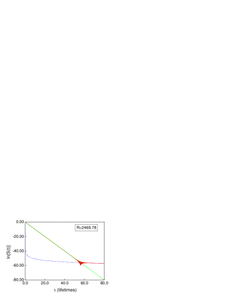
Figure 1: ‘online color’. The Survival probability $S(t)$ (solid line) as a function of time for a double-barrier system with $R$ as indicated and $\tau_{1}=16321.9$ fs. The purely exponential behavior of $S(t)$ (dashed line) and the long-time asymptotic behavior as $t^{-3}$ (dotted line), are included for comparison. See text.

In Fig. 1 we have used a set of potential parameters typical of AlAs-GaAs-AlAs double-barrier heterostructures as in the cases considered by Sakaki and co-workers sakaki , who verified experimentally that electrons in sufficiently thin symmetric double-barrier resonant structures decay proceeds according to the exponential decay law. The potential parameters are: barrier widths $b=2.5$ nm, well width $w=6.2$ nm, and barrier heights $V=1.36$ eV. In the calculations the electron effective mass is $m=0.067m_{e}$, where $m_{e}$ is the bare electron mass. The resonance parameters of the system are: resonance energy $\varepsilon_{1}=0.09959$ eV, resonance width $\Gamma_{1}=4.0325\times 10^{-5}$ eV. Hence $R=\varepsilon_{1}/\Gamma_{1}=2469.78$, much larger than unity, and the lifetime is $\tau_{1}=\hbar/\Gamma_{1}=16321.9$ fs. The survival probability $S(t)$ (solid line) is calculated using Eq. (11). For comparison, Fig. 1 exhibits also $S(t)^{\ell}_{non}$ (dot line), given by Eq. (16), and the purely exponential contribution $\exp(-\Gamma_{1}t/\hbar)$ (dashed line), i.e., Eq. (12) with $C_{1}\bar{C}_{1}=1$. We see that exponential decay law stands for many lifetimes. The long time nonexponential contribution becomes relevant only after $60$ lifetimes when the value of $S(t)$ is extremely small, most possibly beyond experimental verification.

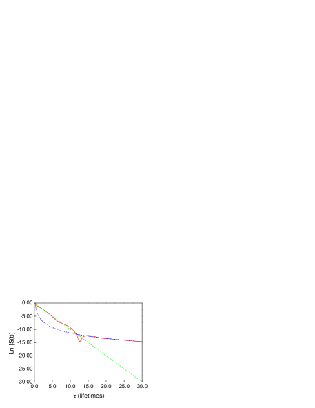
Figure 2: ‘online color’. The Survival probability $S(t)$ (solid line), as a function of time in lifetime units for a double-barrier system exhibiting the transition from exponential to nonexponential behavior. Here $\tau_{1}=10.69$ fs. The purely exponential behavior of $S(t)$ (dashed line) and the long-time asymptotic behavior (dotted line), are included for comparison. See text.

The oscillations of the survival probability around the exponential-nonexponential transition in Fig. 1, are caused by the cosine factor appearing in the interference term $S_{int}$ given by Eq. (14). In the long time limit, i.e., Eq. (17), the cosine factor may be expressed in terms of the parameters $R$ and $\tau$ as $\cos(R\tau+\eta)$, and it explains the extremely large frequency of oscillations of $S(t))$ around the exponential-nonexponential transition for $R>>1$.

By varying the potential parameters, one obtains also that the onset of the exponential-nonexponential transition in lifetime units, depends on the value $R=\varepsilon_{1}/\Gamma_{1}$. In fact, it occurs earlier as $R$ diminishes. This also occurs in the case of the exact single resonance decay formula, whose only input is the value of $R$ gcrr01 . One sees, from the above cosine factor, that the frequency of oscillations diminishes also as $R$ becomes smaller. This is interesting, because it may allow to design structures with appropriate parameters to exhibit nonexponential behavior in ranges more adequate for experiment.

As an example of this, Fig. 2 exhibits a plot of the survival probability $S(t)$ (solid line) in a case where $R=0.91$. The potential parameters of the double-barrier structure are ferry , barrier widths $b=1.0$ nm, well width $w=5.0$ nm, and barrier heights $V=0.23$ eV which give: $\varepsilon_{1}=0.05639$ eV, $\Gamma_{1}=0.06151$ eV and $\tau_{1}=10.69$ fs. The nonexponential behavior is set now around $15$ lifetimes and the value of $S(t)$ is order of magnitudes larger than in the preceding case. Again, for comparison, $S(t)^{\ell}_{non}$ (dot line) and the purely exponential $\exp(-i\Gamma_{1}t/\hbar)$ (dashed line) are plotted. Note also, since $R=0.91$, of the order of unity, that the frequency of oscillations around the exponential-nonexponential transition is much more reduced than in the previous case.

Now, it turns out that by considering systems with still smaller values of $R$, leads to the regime where that decay proceeds entirely in a nonexponential fashion. We have found that this occurs for values $R\lesssim 0.3$ rvalue . Figure 3 illustrates an example of this regime. The potential parameters for the barrier widths and barrier heights remain the same as in the previous case, $b=1.0$ nm and $V=0.23$ eV, but the well width takes now the value $w=1.5$ nm. Note that since each monolayer of semiconductor material has a thickness of about $0.25$ nm barnham , each barrier and the well involve, respectively, $4$ and $6$ monolayers. For this system the resonance parameters are: $\varepsilon_{1}=0.07025$ eV and $\Gamma_{1}=0.40075$ eV. Also $R=0.1753$ and $\tau_{1}=1.64$ fs. Here the real part of the complex pole, $\alpha_{1}=0.0491$ is still larger than the corresponding imaginary part $\beta=.03532$, which means that the pole is proper and provides an exponentially decaying contribution i.e., Eq. (12). Although the resonance width is much broader than the resonance energy, the double-barrier system is still able to trap the particle. One sees that the survival probability $S(t)$ (solid line) exhibits a behavior that departs from the purely exponential behavior $\exp(-i\Gamma_{1}t/\hbar)$ (dashed line) along the full time span. Note that the long time regime, $S(t)_{non})$ (dot line), becomes the dominant contribution only after 15 lifetimes. Hence, one may ask what originates previously the deviation of $S(t)$ from the exponential behavior. The answer follows by inspection of the expression for $S(t)$ given by Eq. (11): the deviation from exponential behavior is due to the interference term $S(t)_{int}$.

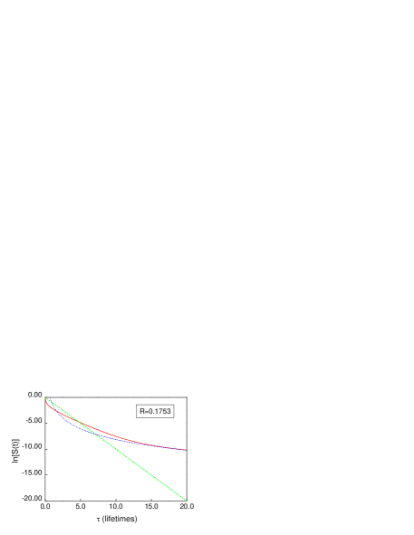
Figure 3: ‘online color’. Full nonexponential behavior of the survival probability $S(t)$ (solid line), for a double-barrier system as a function of time. Here $\tau_{1}=1.64$ fs. The purely exponential behavior for $S(t)$ (dashed line), and the long time asymptotic behavior of $S(t)$ (dotted line), are included for comparison. See text.

This is illustrated in Fig. 4. The interference term $S(t)_{int}$ (dashed-dot line), given by Eq. (14), adds up a negative contribution to the exponential decaying contribution $S(t)_{exp}$ (dashed line) given by Eq. (12), to yield a nonexponential behavior of the survival probability $S(t)$ (solid line) in a time span that for larger values of $R$ is usually dominated by the exponential term.

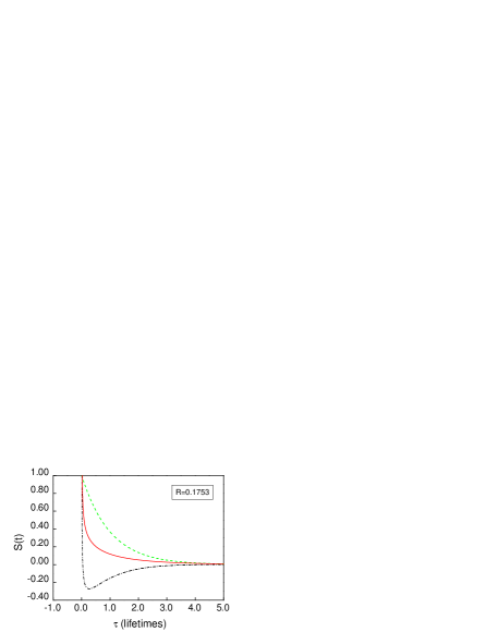
Figure 4: ‘online color’. Survival probability $S(t)=S(t)_{exp}+S(t)_{non}+S(t)_{int}$ (solid line) for a few lifetimes to show that $S(t)_{int}$ (dashed-dot line) causes the deviation from the exponential contribution $S(t)_{exp}$ (dashed line) in the pre-asymptotic regime for the same case of Fig. 3. See text.

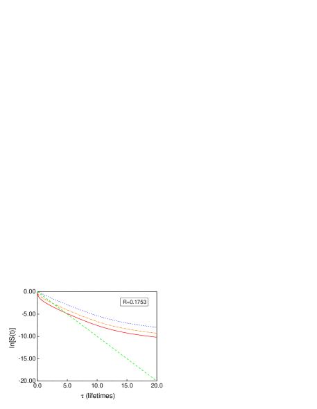
Figure 5: ‘online color’. The survival probability $S(t)$ for different initial states: infinite box (solid line), exact single resonance (dot-dashed line) and resonant function $u_{1}(x)$ (dotted line). For comparison, the purely exponential behavior is also plotted (dashed line). See text.

As pointed out before, in the above calculations we have considered as initial state a box solution of well width $w$. We have examined different choices of the initial state to see how the nonexponential behavior of the survival probability is affected. We have found some quantitative differences but the nonexponential behavior remains unaffected. The differences arise from the distinct values of the expansion coefficients as illustrated in Fig. 5 for $R=0.1753$, where we compare: (a) the box initial solution (solid line) $[{\rm Re}\,(C_{1}{\bar{C}}_{1})=0.611]$, (b) the analytical exact single level resonance formulagcrr01 (dash-dotted line) $[{\rm Re}\,(C_{1}{\bar{C}}_{1})=1.0]$, and, (c) the case where the initial state is the resonance function $u_{1}(x)$ along the internal region of the structure (dotted line) $[{\rm Re}\,(C_{1}{\bar{C}}_{1})=2.070]$.

We believe that a possible way to test our results for the full time nonexponential behavior of quantum decay, is by means of an experimental setup analogous to that used by Sakaki et al. sakaki where a laser is used to create electron-heavy-hole pairs in the quantum well of the double barrier. For thin barriers, as in the example discussed here, these authors showed that the decay process is dominated by tunneling escape compared with the competing radiative recombination process. The decay rate of electrons is then measured indirectly by analyzing the time-resolved photoluminescence. What is relevant here is that the value of $R=\varepsilon_{1}/\Gamma_{1}\leq 0.3$. Clearly these values of $R$ may be designed in other artificial quantum structures as in the decay of trapped atoms by lasers raizen .

On completing this work it came to our notice a very recent work by Rothe et.al. rothe , where it is reported the long-awaited experimental verification of the deviation of the exponential decay law at long times. This has been achieved by measuring luminescence decays of dissolved organic materials. A distinctive feature of this work is that the small value of $R$ is induced by a local solvent environment. In this respect this work differs from our approach which refers to the decay of an isolated system. It is to be expected that this experimental work will stimulate further research in this area.

IV Concluding remarks

In summary, we have found that the full time nonexponential behavior of the survival probability may be also characterized by three regimes: (a)  A first regime, encompassing a small fraction of the lifetime of the system, that is dominated by the short-time behavior and the high resonance contributions to the survival probability; (b) A second regime, dominated by the interference contribution between the exponential and the nonexponential terms to the survival probability;  (c) A third regime that is dominated by the long time asymptotic nonexponential contribution to decay. In fact, (a) and (c) are regimes that are present in general in any decaying system. The nonexponential behavior of decay in stage (b) appears in systems with a small value of the parameter $R$ in the range $0<R\lesssim\ 0.3$. For larger values of $R$ this regime corresponds to the usual exponentially decaying behavior. Our approach possesses a general character for decay in quantum systems, and therefore, it may be applied to study the transition from exponential to nonexponential decay, and in particular the purely nonexponential regime, in other suitable designed artificial quantum structures.

- (1) G. Gamow, Z. Phys. 51, 204-212 (1928); G. Gamow and C. L. Critchfield, Theory of Atomic Nucleus and Nuclear Energy-Sources (Oxford University Press, London, 1949).
- (2) R. W. Gurney and E. U. Condon, Phys. Rev. 33 127 (1929).
- (3) L. A. Khalfin, Sov. Phys. JETP 6, 1053-1063 (1958).
- (4) P. Exner, Open Quantum Systems and Feynman Integrals (Reidel, Dordrecht, 1985).
- (5) D. S. Onley and A. Kumar, Am. J. Phys. 60, 432 (1992).
- (6) J. G. Muga, G. W. Wei, and R. F. Snider, Ann. Phys. 252 336 (1996).
- (7) P. T. Greenland, Nature 335, 298 (1988); Nature 387, 548 (1997).
- (8) D. A. Dicus, W. W. Wayne, R. F. Schwitters and T. M. Tinsley, Phys. Rev. A 65, 032116 (2002).
- (9) E. Rufeil and H. M. Pastawski, Chem. Phys. Lett. 420, 35 (2006).
- (10) E. B. Norman, S. B. Gazes, S. G. Crane and D. A. Bennett, Phys. Rev. Lett. 60 2246 (1988); E. B. Norman, B. Sur, K. T. Lesko, R-M. Lammer, D. J. DePaolo and T. L. Owens, Phys. Lett. B 357 521 (1995).
- (11) OPAL Collaboration, G. Alexander et.el., Phys. Lett. B 368, 244 (1996).
- (12) S. R. Wilkinson, C. F. Bharucha, M. C. Fischer, K. W. Madison, P. K. Morrow, Q. Niu, B. Sundaram and M G. Raizen, Nature 387 575 (1997).
- (13) G. García-Calderón, V. Riquer, and R. Romo, J. Phys. A 34 4155 (2001). See in particular Fig. (2).
- (14) Here and in the rest of the discussion we take the threshold energy . Otherwise, .
- (15) T. Jittoh, S. Matsumoto, J. Sato, Y. Sato, and K. Takeda, Phys. Rev. A 71 012109 (2005).
- (16) R. G. Newton, Scattering Theory of Waves and Particles. 2nd. Ed. (Springer-Verlag, New York, 1982).
- (17) G. García-Calderón in Symmetries in Physics, edited by A. Frank and K. B. Wolf (Springer-Verlag, Berlin, 1992) p.252; See also, G. García-Calderón, J. L. Mateos, and M. Moshinsky, Phys. Rev. Lett. 74, 337 (1995).
- (18) For the properties of resonance functions in one dimension, see for example, G. García-Calderón and A. Rubio, Phys. Rev. A 55, 3361 (1997).
- (19) M. Abramowitz and I. A. Stegun, Handbook of Mathematical Functions, (Dover Publications, Inc. New York, 1965) p. 297.
- (20) M. Tsuchiya, T. Matsusue, and H. Sakaki, Phys. Rev. Lett. 59, 2356 (1987).
- (21) D. K. Ferry and S. M. Goodnick, Transport in Nanostructures, (Cambridge University Press, United Kingdom, 1997).
- (22) This is slightly smaller than the estimate given in Ref. jittoh, .
- (23) E. A. Johnson, in Low-Dimensional Semiconductor Structures, Fundamentals and Device Applications, edited by K. Barnham and D. Vvedensky (Cambridge University Press, 2001)p. 56.
- (24) C. Rothe, S. I., Hintschich and A. P. Monkman, Phys. Rev. Lett. 96, 163601 (2006).