Existence of A Rigorous Density-Functional Theory for Open Electronic Systems

Abstract

We prove that the electron density function of a real physical system can be uniquely determined by its values on any finite subsystem. This establishes the existence of a rigorous density-functional theory for any open electronic system. By introducing a new density functional for dissipative interactions between the reduced system and its environment, we subsequently develop a time-dependent density-functional theory which depends in principle only on the electron density of the reduced system.

Density-functional theory (DFT) has been widely used as a research tool in condensed matter physics, chemistry, materials science, and nanoscience. The Hohenberg-Kohn theorem hk lays the foundation of DFT. The Kohn-Sham formalism ks provides a practical solution to calculate the ground state properties of electronic systems. Runge and Gross extended DFT further to calculate the time-dependent properties and hence the excited state properties of any electronic systems tddft . The accuracy of DFT or time-dependent DFT (TDDFT) is determined by the exchange-correlation functional. If the exact exchange-correlation functional were known, the Kohn-Sham formalism would have provided the exact ground state properties, and the Runge-Gross extension, TDDFT, would have yielded the exact time-dependent and excited states properties. Despite their wide range of applications, DFT and TDDFT have been mostly limited to isolated systems.

Many systems of current research interest are open systems. A molecular electronic device is one such system. DFT-based simulations have been carried out on such devices prllang ; prlheurich ; jcpluo ; langprb ; prbguo ; jacsywt ; jacsgoddard ; transiesta ; jcpratner . These simulations focus on steady-state currents under bias voltages. Two types of approaches have been adopted. One is the Lippmann-Schwinger formalism by Lang and coworkers langprb . The other is the first-principles nonequilibrium Green’s function (NEGF) technique prbguo ; jacsywt ; jacsgoddard ; transiesta ; jcpratner . In both approaches the Kohn-Sham Fock operator is taken as the effective single-electron model Hamiltonian, and the transmission coefficients are calculated within the noninteracting electron model. The investigated systems are not in their ground states, and applying ground state DFT formalism for such systems is only an approximation cpdatta . DFT formalisms adapted for current-carrying systems have also been proposed recently, such as Kosov’s Kohn-Sham equations with direct current jcpkosov and Burke et al.’s Kohn-Sham master equation including dissipation to phonons prlburke . However, practical implementation of these formalisms requires the electron density function of the entire system. In this paper, we present a rigorous DFT formalism for any open electronic system. The first-principles formalism depends in principle only on the electron density function of the reduced system, and can be used to simulate the transient electronic response.

It is often implicitly assumed that the electron density function of any real physical system is real analytic ourarxiv . This is reflected in many existing first-principles methodologies. In practical quantum mechanical simulations, real analytic functions such as Gaussian functions, Slater functions and plane wave functions are adopted as basis sets, which results in real analytic electron density distribution. However, analyticity is not guaranteed for all presently used basis functions. For instance, in the linearized augmented plane wave (LAPW) method booklapw , radial functions times spherical harmonics span the inside of muffin-tin spheres whereas plane waves are used for the interstitial regime. By this approximation the electron density cannot be analytically continued across the interface of the two disconnected parts. It is thus interesting to ask whether the electron density function of any real system is in principle real analytic. This question was settled recently for time-independent systems.

Fournais et al. proved that the electron densities of atomic and molecular eigenfunctions are real analytic in $\mathbf{r}$-space away from the nuclei analyticity . Their proof is based on the fact that the time-independent Schrödinger equation, $\hat{H}\Psi=E\Psi$, is an elliptic partial differential equation, and its eigenfunctions can always be real analytic (except isolated points) and quadratically integrable. Their rigorous proof implies that the electron density function of a real physical system is real analytic (except at nuclei) when the system in its ground state, any of its excited eigenstates, or any state which is a linear combination of finite number of its eigenstates. In their derivation analyticity , nuclei are treated as point charges, and this leads to non-analytic electron density at these isolated points. Note that the isolated points at nuclei can be excluded for the moment from the physical space that we consider, so long as the space is connected. Later we will come back to these isolated points, and show that their inclusion does not alter our results. We show now that for a time-independent real physical system the electron density distribution function in a sub-space determines uniquely its values on the entire physical space. This is nothing but analytic continuation of a real analytic function. The proof for univariable real analytical functions can be found in textbooks, for instance, Ref. proof1 . The extension to multivariable real analytical functions is straightforward.

Lemma : The electron density function $\rho(\mathbf{r})$ is real analytic in a connected physical space $U$. $D\subseteq U$ is a sub-space. If $\rho(\mathbf{r})$ is known for all $\mathbf{r}\in D$, $\rho(\mathbf{r})$ can be uniquely determined on the entire space $U$.

Proof: To facilitate our discussion, the following notations are introduced. Set $\mathbb{Z}^{+}=\{0,1,2,\ldots\}$, and $\gamma$ is an element of $(\mathbb{Z}^{+})^{3}$, i.e., $\gamma=(\gamma_{1},\gamma_{2},\gamma_{3})\in(\mathbb{Z}^{+})^{3}$. The displacement vector $\mathbf{r}$ is denoted by the three-dimensional variable $x=(x_{1},x_{2},x_{3})\in U$. Denote that $\gamma\,\mbox{!}=\gamma_{1}\,\mbox{!}\>\gamma_{2}\,\mbox{!}\>\gamma_{3}\,\mbox{!}\,$, $x^{\gamma}=x_{1}^{\gamma_{1}}\>x_{2}^{\gamma_{2}}\>x_{3}^{\gamma_{3}}$, and $\frac{\partial^{\gamma}}{\partial x^{\gamma}}=\frac{{\partial}^{\gamma_{1}}}{\partial x_{1}^{\gamma_{1}}}\frac{\partial^{\gamma_{2}}}{\partial x_{2}^{\gamma_{2}}}\frac{\partial^{\gamma_{3}}}{\partial x_{3}^{\gamma_{3}}}$.

Suppose that another density distribution function $\rho^{\prime}(x)$ is real analytic in $U$ and equal to $\rho(x)$ for all $x\in D$. We have $\frac{\partial^{\gamma}\rho(x)}{\partial x^{\gamma}}=\frac{\partial^{\gamma}\rho^{\prime}(x)}{\partial x^{\gamma}}$ for all $x\in D$ and $\gamma\in(\mathbb{Z}^{+})^{3}$. Taking a point $x_{0}\in D$ and at or infinitely close to the boundary of $D$, we may expand $\rho(x)$ and $\rho(x^{\prime})$ around $x_{0}$, i.e., $\rho(x)=\sum_{\gamma\in(\mathbb{Z}^{+})^{3}}\frac{1}{\gamma!}\left.\frac{\partial^{\gamma}\rho(x)}{\partial x^{\gamma}}\right|_{x_{0}}(x-x_{0})^{\gamma}$ and $\rho^{\prime}(x)=\sum_{\gamma\in(\mathbb{Z}^{+})^{3}}\frac{1}{\gamma!}\left.\frac{\partial^{\gamma}\rho^{\prime}(x)}{\partial x^{\gamma}}\right|_{x_{0}}(x-x_{0})^{\gamma}$. Assuming that the convergence radii for the Taylor expansions of $\rho(x)$ and $\rho^{\prime}(x)$ at $x_{0}$ are both larger than a positive finite real number $b$, we have thus $\rho(x)=\rho^{\prime}(x)$ for all $x\in D_{b}(x_{0})=\left\{x:\left|x-x_{0}\right|<b\right\}$ since $\left.\frac{\partial^{\gamma}\rho(x)}{\partial x^{\gamma}}\right|_{x_{0}}=\left.\frac{\partial^{\gamma}\rho^{\prime}(x)}{\partial x^{\gamma}}\right|_{x_{0}}$. Therefore, the equality $\rho^{\prime}(x)=\rho(x)$ has been expanded beyond $D$ to include $D_{b}(x_{0})$. Since $U$ is connected the above procedures can be repeated until $\rho^{\prime}(x)=\rho(x)$ for all $x\in U$. We have thus proven that $\rho$ can be uniquely determined in $U$ once it is known in $D$.

With the above Lemma we are ready to prove the following theorem:

Theorem 1: A connected time-independent real physical system is in the ground state. The electron density function $\rho(\mathbf{r})$ of any finite subsystem determines uniquely all electronic properties of the entire system.

Proof: Assuming the physical spaces spanned by the subsystem and the connected real physical system are $D$ and $U$, respectively. $D$ is thus a sub-space of $U$, i.e., $D\subseteq U$. According to the above lemma, $\rho(\mathbf{r})$ in $D$ determines uniquely its values in $U$, i.e., $\rho(\mathbf{r})$ of the subsystem determines uniquely $\rho(\mathbf{r})$ of the entire system.

Inclusion of isolated points, lines or planes where $\rho(\mathbf{r})$ is non-analytic into the connected physical space does not violate the above conclusion, so long as $\rho(\mathbf{r})$ is continuous at these points, lines or planes. This can be shown clearly by performing analytical continuation of $\rho(\mathbf{r})$ infinitesimally close to them. Therefore, $\rho(\mathbf{r})$ of any finite subsystem determines uniquely $\rho(\mathbf{r})$ of the entire physical system including nuclear sites. Hohenberg-Kohn theorem hk states that the ground state electron density distribution of any system determines uniquely all its electronic properties. Hence we conclude that ground state $\rho(\mathbf{r})$ of any finite subsystem determines all the electronic properties of the entire real physical system.

As for time-dependent systems, the issue is less clear. Although it seems intuitive that the electron density function of any time-dependent real physical system is real analytical (except isolated points in space-time), it turns out quite difficult to prove the analyticity rigorously. Fortunately we are able to establish a one-to-one correspondence between the electron density function of any finite subsystem and the external potential field which is real analytical in both $t$-space and $\mathbf{r}$-space, and thus circumvent the difficulty concerning the analyticity of time-dependent electron density function. For time-dependent real physical systems, we have the following theorem:

Theorem 2: The electron density function of a real physical system at $t_{0}$, $\rho(\mathbf{r},t_{0})$, is real analytic in $\mathbf{r}$-space, and the corresponding wave function is $\Phi(t_{0})$. The system is subjected to a real analytic (in both $t$-space and $\mathbf{r}$-space) external potential field $v(\mathbf{r},t)$. Let $D$ be a finite $\mathbf{r}$-subspace. The time-dependent electron density function on the subspace $D$, $\rho(\mathbf{r},t)$ with $\mathbf{r}\in D$, has thus a one-to-one correspondence with $v(\mathbf{r},t)$ and determines uniquely all electronic properties of the entire time-dependent system.

Proof: Let $v(\mathbf{r},t)$ and $v^{\prime}(\mathbf{r},t)$ be two real analytical potentials in both $t$-space and $\mathbf{r}$-space which differ by more than a constant at any time $t\geqslant t_{0}$, and their corresponding electron density functions are $\rho(\mathbf{r},t)$ and $\rho^{\prime}(\mathbf{r},t)$, respectively. Therefore, there exists a minimal nonnegative integer $k$ such that the $k$-th order derivative differentiates these two potentials at $t_{0}$:

$$\left.\frac{\partial^{k}}{\partial t^{k}}\left[v(\mathbf{r},t)-v^{\prime}(\mathbf{r},t)\right]\right|_{t=t_{0}}\neq\mbox{const}.$$ (1)

Following exactly the Eqs. (3)-(6) of Ref. tddft , we have

$$\left.\frac{\partial^{k+2}}{\partial t^{k+2}}\left[\rho(\mathbf{r},t)-\rho^{\prime}(\mathbf{r},t)\right]\right|_{t=t_{0}} = -\nabla\cdot u(\mathbf{r}),$$ (2)

where

$$u(\mathbf{r}) = \rho(\mathbf{r},t_{0})\,\nabla\!\left\{\left.\frac{\partial^{k}}{\partial t^{k}}\left[v(\mathbf{r},t)-v^{\prime}(\mathbf{r},t)\right]\right|_{t=t_{0}}\right\}.$$ (3)

Due to the analyticity of $\rho(\mathbf{r},t_{0})$, $v(\mathbf{r},t)$ and $v^{\prime}(\mathbf{r},t)$, $\nabla\cdot u(\mathbf{r})$ is also real analytic in $\mathbf{r}$-space. It has been proven in Ref. tddft that it is impossible to have $\nabla\cdot u(\mathbf{r})=0$ on the entire $\mathbf{r}$-space. Therefore it is also impossible that $\nabla\cdot u(\mathbf{r})=0$ everywhere in $D$ (otherwise based on the Lemma proven earlier, $\nabla\cdot u(\mathbf{r})$ can always be analytically continued from the particular finite $\mathbf{r}$-subspace where its values are $0$ to the entire $\mathbf{r}$-space, and this would lead to $\nabla\cdot u(\mathbf{r})=0$ everywhere in the entire $\mathbf{r}$-space). We have thus

$$\left.\frac{\partial^{k+2}}{\partial t^{k+2}}\left[\rho(\mathbf{r},t)-\rho^{\prime}(\mathbf{r},t)\right]\right|_{t=t_{0}} \neq 0$$ (4)

for $\mathbf{r}\in D$. This confirms the existence of a one-to-one correspondence between $v(\mathbf{r},t)$ and $\rho(\mathbf{r},t)$ with $\mathbf{r}\in D$. $\rho(\mathbf{r},t)$ on the subspace $D$ thus determines uniquely all electronic properties of the entire system. This completes the proof of Theorem 2.

Note that if $\Phi(t_{0})$ is the ground state, any excited eigenstate, or any state as a linear combination of finite number of eigenstates of a time-independent Hamiltonian, the prerequisite condition in Theorem 2 that the electron density function $\rho(\mathbf{r},t_{0})$ be real analytic is automatically satisfied, as proven in Ref. analyticity . As long as the electron density function at $t=t_{0}$, $\rho(\mathbf{r},t_{0})$, is real analytic, it is guaranteed that $\rho(\mathbf{r},t)$ on the subsystem $D$ determines all physical properties of the entire system at any time $t$ if the external potential $v(\mathbf{r},t)$ is real analytic.

According to Theorem 1 and 2, the electron density function of any subsystem determines all the electronic properties of the entire time-independent or time-dependent physical system. This proves in principle the existence of a rigorous DFT-type formalism for open electronic systems. All one needs to know is the electron density of the reduced system. The challenge that remains is to develop a practical first-principles formalism.

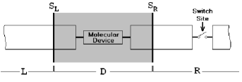
Figure 1: Schematic representation of the experimental setup for quantum transport through a molecular device.

Fig. 1 depicts an open electronic system. Region $D$ containing a molecular device is the reduced system of our interests, and the electrodes $L$ and $R$ are the environment. Altogether $D$, $L$ and $R$ form the entire system. Taking Fig. 1 as an example, we develop a practical DFT formalism for the open systems. Within the TDDFT formalism, a closed equation of motion (EOM) has been derived for the reduced single-electron density matrix $\sigma(t)$ of the entire system ldmtddft :

$$i\dot{\sigma}(t)=[h(t),\sigma(t)],$$ (5)

where $h(t)$ is the Kohn-Sham Fock matrix of the entire system, and the square bracket on the right-hand side (RHS) denotes a commutator. The matrix element of $\sigma$ is defined as $\sigma_{ij}(t)=\langle a^{\dagger}_{j}(t)\,a_{i}(t)\rangle$, where $a_{i}(t)$ and $a^{\dagger}_{j}(t)$ are the annihilation and creation operators for atomic orbitals $i$ and $j$ at time $t$, respectively. Fourier transformed into frequency domain while considering linear response only, Eq. (5) leads to the conventional Casida’s equation casida . Expanded in the atomic orbital basis set, the matrix $\sigma$ can be partitioned as:

$$\sigma=\left[\begin{array}[]{lll}\sigma_{L}&\sigma_{LD}&\sigma_{LR}\\ \sigma_{DL}&\sigma_{D}&\sigma_{DR}\\ \sigma_{RL}&\sigma_{RD}&\sigma_{R}\end{array}\right],$$ (6)

where $\sigma_{L}$, $\sigma_{R}$ and $\sigma_{D}$ represent the diagonal blocks corresponding to the left lead $L$, the right lead $R$ and the device region $D$, respectively; $\sigma_{LD}$ is the off-diagonal block between $L$ and $D$; and $\sigma_{RD}$, $\sigma_{LR}$, $\sigma_{DL}$, $\sigma_{DR}$ and $\sigma_{RL}$ are similarly defined. The Kohn-Sham Fock matrix $h$ can be partitioned in the same way with $\sigma$ replaced by $h$ in Eq. (6). Thus, the EOM for $\sigma_{D}$ can be written as

$$i\dot{\sigma}_{D} = [h_{D},\sigma_{D}]+\sum_{\alpha=L,R}\left(h_{D\alpha}\sigma_{\alpha D}-\sigma_{D\alpha}h_{\alpha D}\right)$$ (7)

$$= [h_{D},\sigma_{D}]-i\sum_{\alpha=L,R}Q_{\alpha},$$

where $Q_{L}$ ($Q_{R}$) is the dissipative term due to $L$ ($R$). With the reduced system $D$ and the leads $L/R$ spanned respectively by atomic orbitals $\{l\}$ and single-electron states $\{k_{\alpha}\}$, Eq. (7) is equivalent to:

$$i\dot{\sigma}_{nm} = \sum_{l\in D}\,(h_{nl}\sigma_{lm}-\sigma_{nl}h_{lm})-i\sum_{\alpha=L,R}Q_{\alpha,nm},$$ (8)

$$Q_{\alpha,nm} = i\sum_{k_{\alpha}\in\alpha}\big{(}h_{nk_{\alpha}}\sigma_{k_{\alpha}m}-\sigma_{nk_{\alpha}}h_{k_{\alpha}m}\big{)},$$ (9)

where $m$ and $n$ correspond to the atomic orbitals in region $D$; $k_{\alpha}$ corresponds to an electronic state in the electrode $\alpha$ ($\alpha=L$ or $R$). $h_{nk_{\alpha}}$ is the coupling matrix element between the atomic orbital $n$ and the electronic state $k_{\alpha}$. The current through the interfaces $S_{L}$ or $S_{R}$ (see Fig. 1) can be evaluated as follows,

$$J_{\alpha}(t) = -\int_{\alpha}d\mathbf{r}\,\frac{\partial}{\partial t}\rho(\mathbf{r},t)$$ (10)

$$= -\sum_{k_{\alpha}\in\alpha}\frac{d}{dt}\,\sigma_{k_{\alpha}k_{\alpha}}\!(t)$$

$$= i\sum_{l\in D}\sum_{k_{\alpha}\in\alpha}\big{(}h_{k_{\alpha}l}\,\sigma_{lk_{\alpha}}-\sigma_{k_{\alpha}l}\,h_{lk_{\alpha}}\big{)}$$

$$= -\sum_{l\in D}Q_{\alpha,ll}=-\mbox{tr}\big{[}Q_{\alpha}(t)\big{]},$$

i.e., the trace of $Q_{\alpha}$.

At first glance Eq. (8) is not self-closed since the dissipative terms $Q_{\alpha}$ remain unsolved. According to Theorem 1 and 2, all physical quantities are explicit or implicit functionals of the electron density of the reduced system $D$, $\rho_{D}(\mathbf{r},t)$. Note that $\rho_{D}(\mathbf{r},t)=\rho(\mathbf{r},t)$ for $\mathbf{r}\in D$. $Q_{\alpha}$ is thus also a universal functional of $\rho_{D}(\mathbf{r},t)$. Therefore, Eq. (8) can be recast into a formally closed form,

$$\!\!i\dot{\sigma_{D}}=\Big{[}h_{D}[\mathbf{r},t;\rho_{D}(\mathbf{r},t)],\sigma_{D}\Big{]}-i\!\!\sum_{\alpha=L,R}\!\!Q_{\alpha}[\mathbf{r},t;\rho_{D}(\mathbf{r},t)].$$ (11)

Neglecting the second term on the RHS of Eq. (11) leads to the conventional TDDFT formulation in terms of reduced single-electron density matrix ldmtddft for the isolated reduced system. The second term describes the dissipative processes between $D$ and $L$ or $R$. Besides the exchange-correlation functional, an additional universal density functional, the dissipation functional $Q_{\alpha}[\mathbf{r},t;\rho_{D}(\mathbf{r},t)]$, is introduced to account for the dissipative interaction between the reduced system and its environment. Eq. (11) is the TDDFT EOM for open electronic systems. Burke et al. extended TDDFT to include electronic systems interacting with phonon baths prlburke , they proved the existence of a one-to-one correspondence between $v(\mathbf{r},t)$ and $\rho(\mathbf{r},t)$ under the condition that the dissipative interactions (denoted by a superoperator $\mathcal{C}$ in Ref. prlburke ) between electrons and phonons are fixed. In our case since the electrons can move in and out the reduced system, the number of the electrons in the reduced system is not conserved. In addition, the dissipative interactions can be determined in principle by the electron density of the reduced system. We do not need to stipulate that the dissipative interactions with the environment are fixed as Burke et al.. And the only information we need is the electron density of the reduced system. In the frozen DFT approach warshel an additional exchange-correlation functional term was introduced to account for the exchange-correlation interaction between the system and the environment. This additional term is included in $h_{D}[\mathbf{r},t;\rho_{D}(\mathbf{r},t)]$ of Eq. (11). An explicit form of the dissipation functional $Q_{\alpha}$ is required for practical implementation of Eq. (11). Admittedly $Q_{\alpha}[\mathbf{r},t;\rho_{D}(\mathbf{r},t)]$ is an extremely complex functional and difficult to evaluate. As various approximated expressions have been adopted for the DFT exchange-correlation functional in practical implementations, the same strategy can be applied to the dissipation functional $Q_{\alpha}$. Work along this direction will be published elsewhere longpaper .

Given $Q_{\alpha}[\rho]$ how do we solve Eq. (11) in practice? Again take the molecular device shown in Fig. 1 as an example. We may integrate Eq. (11) directly by satisfying the boundary conditions at $S_{L}$ and $S_{R}$. The only boundary condition we need is the potentials at $S_{L}$ and $S_{R}$. We need thus integrate Eq. (11) together with a Poisson equation for Coulomb potential. And the Poisson equation is subjected to the boundary condition determined by the potentials at $S_{L}$ and $S_{R}$. It is important to point out that although in principle its physical span can be small, in practice the reduced system is to be chosen so that Eq. (11) can be solved readily with convenient boundary conditions. For instance, for the molecular electronic device depicted in Fig. 1, the reduced system $D$ contains not only the molecular device itself, but also portions of the left and right electrodes. In this way the Coulomb potential at the boundary take approximately the values of the bulk leads.

To summarize, we have proved rigorously the existence of a first-principles method for both time-independent and time-dependent open electronic systems, and developed a formally closed TDDFT formalism by introducing a new dissipation functional. This new functional $Q_{\alpha}$ depends only on the electron density function of the reduced system. With an explicit form for the universal dissipation functional $Q_{\alpha}$, the time evolution of an open electron system in external fields is fully characterized by Eq. (11). In practical calculations, we need thus focus only on the reduced system with appropriate boundary conditions. This work greatly extends the realm of density-functional theory.

- (1)
- (2) P. Hohenberg and W. Kohn, Phys. Rev. 136, B 864, (1964)
- (3) W. Kohn and L. J. Sham, Phys. Rev. 140, A 1133 (1965)
- (4) E. Runge and E. K. U. Gross, Phys. Rev. Lett. 52, 997 (1984)
- (5) N. D. Lang and Ph. Avouris, Phys. Rev. Lett. 84, 358 (2000)
- (6) J. Heurich, J. C. Cuevas, W. Wenzel and G. Schön, Phys. Rev. Lett. 88, 256803 (2002)
- (7) C.-K. Wang and Y. Luo, J. Chem. Phys. 119, 4923 (2003)
- (8) N. D. Lang, Phys. Rev. B 52, 5335 (1995)
- (9) Y. Xue, S. Datta and M. A. Ratner, J. Chem. Phys. 115, 4292 (2001)
- (10) J. Taylor, H. Guo and J. Wang, Phys. Rev. B. 63, 245407 (2001)
- (11) S.-H. Ke, H. U. Baranger and W. Yang, J. Am. Chem. Soc. 126, 15897 (2004)
- (12) W.-Q. Deng, R. P. Muller and W. A. Goddard III, J. Am. Chem. Soc. 126, 13563 (2004)
- (13) M. Brandbyge et al., Phys. Rev. B 65, 165401 (2002)
- (14) Y. Xue, S. Datta and M. A. Ratner, Chem. Phys. 281, 151 (2002)
- (15) D. S. Kosov, J. Chem. Phys. 119, 1 (2003)
- (16) K. Burke, R. Car and R. Gebauer, Phys. Rev. Lett. 94, 146803 (2005)
- (17) X. Zheng and G.H. Chen, arXiv:physics/0502021 (2005)
- (18) D. Singh, Plane Waves, Pseudopotentials and the LAPW Method, Kluwer Academic (1994)
- (19) S. Fournais, M. Hoffmann-Ostenhof and T. Hoffmann-Ostenhof, Commun. Math. Phys. 228, 401 (2002); S. Fournais, M. Hoffmann-Ostenhof, T. Hoffmann-Ostenhof and T. Ø. Sørensen, Ark. Mat. 42, 87 (2004)
- (20) S. G. Krantz and H. R. Parks, A Primer of Real Analytic Functions, Birkhuser Boston (2002)
- (21) C. Y. Yam, S. Yokojima and G.H. Chen, J. Chem. Phys. 119, 8794 (2003); Phys. Rev. B 68, 153105 (2003)
- (22) M. E. Casida, Recent Developments and Applications in Density Functional Theory, Elsevier, Amsterdam (1996)
- (23) T. A. Wesolowski and A. Warshel, J. Phys. Chem. 97, 8050 (1993)
- (24) X. Zheng, F. Wang and G.H. Chen, to be submitted