Local-field correction to the spontaneous decay rate of atoms
embedded in bodies of finite size

Abstract

The influence of the size and shape of a dispersing and absorbing dielectric body on the local-field corrected spontaneous-decay of an excited atom embedded in the body is studied on the basis of the real-cavity model. By means of a Born expansion of the Green tensor of the system it is shown that to linear order in the susceptibility of the body the decay rate exactly follows Tomaš’s formula found for the special case of an atom at the center of a homogeneous dielectric sphere [Phys. Rev. A 63, 053811 (2001)]. It is further shown that for an atom situated at the interior of an arbitrary dielectric body this formula remains valid beyond the linear order. The case of an atom embedded in a weakly polarizable sphere is discussed in detail.

I Introduction

It has long been recognized that when an atom is situated in a material medium, the local electromagnetic field acting on it differs from the macroscopic one due to the gaps between the atom and the surrounding medium atoms, which are ignored on a coarse-grained macroscopic scale Lorentz1880 ; Onsager36 . Accounting for the difference between the two fields hence requires a correction—the local-field correction. Classical calculations of local-field effects, which typically have their origin in near dipole-dipole interactions, can be found in textbooks (see, e.g., Ref. Lorentz52 ). In quantum theory, investigations of local-field effects are often related to the problem of the spontaneous decay of an excited guest atom embedded in a (dielectric) host. Local-field effects in spontaneous decay have been studied, e.g., for crystals Knoester80 ; Vries98 and disordered dielectrics Juzeliunas97 ; Fleischhauer99 ; Crenshaw00 ; Berman04 on the basis on microscopic models for coupled atomic dipoles.

In macroscopic descriptions, local-field effects are frequently taken into account by regarding the guest atom as being enclosed in a virtual Lorentz1880 ; Scheel99a or real (spherical) cavity Onsager36 ; Glauber91 ; Scheel99b ; Tomas01 ; Rahmani02 ; Ho03 surrounded by the medium, with the cavity size being small compared to the relevant transition wavelength. The cavity in the former model is virtual in the sense that it does not perturb the macroscopic field. It is filled by the atoms comprising the medium, which produce no net effect at the central position in important special cases such as cubic or random structures. In the latter model, the field is modified by the presence of the cavity, which is an empty region containing only the guest atom. Microscopic models often tend to agree with the virtual-cavity results Knoester80 ; Juzeliunas97 ; Fleischhauer99 ; Berman04 , while many recent experiments on spontaneous emission in dielectrics support the real-cavity model Rikken95 ; Lavallard96 ; Schuurmans98 ; Kumar03 . It has been presumed that while the virtual-cavity model applies to interstitial atoms, the real-cavity model is specific to substitutional atoms, and that the case of substitutional atoms occurs prevalently for impurity atoms in disordered dielectrics Vries98 .

Since in the approaches to the local-field effects, the host medium has typically been assumed to be a bulk medium that extends homogeneously to infinity, the question of the effect of the size and shape of the host medium on the local field has arisen. In a macroscopic approach, the spontaneous-decay rate of an excited atom in some free-space region can be given in terms of the imaginary part of the Green tensor of the macroscopic Maxwell equations, which characterizes the (macroscopic) environment of the atom. This relation in principle allows for including local-field corrections for atoms embedded in arbitrary material configurations by assuming a real (spherical) cavity surrounding the atom and calculating the corresponding Green tensor. Using the real-cavity model, Tomaš Tomas01 studied the local-field correction to the spontaneous-decay rate of an excited atom, which is located at the center of a dispersing and absorbing dielectric sphere. Reformulating the result by representing it in a form, which does not explicitly refer to the highly symmetric system considered, he made the conjecture that it may also remain valid beyond the specific example and hence also apply to other locations of the atom and other shapes of the host body.

Based on a numerical computation of the respective Green tensors, Rahmani and Bryant Rahmani02 considered the case of an atom at an arbitrary location within a dielectric sphere or a dielectric cube. Comparing their results for the dielectric sphere including the local-field correction with earlier results disregarding the local-field correction Chew88 ; Kim88 , they suggested a rate formula, which in the case of weakly absorbing material corresponds to Tomaš’s formula. However, since their approach relies heavily on numerical calculations, it cannot produce explicit expressions for the quantities that are related to the local-field correction.

The exact analytical evaluations of the Green tensors of realistic systems which have finite sizes and include a cavity can be very cumbersome. In this paper, we present an attempt to overcome this difficulty by writing the Green tensor as a Born series in terms of the susceptibility, where in many situations one can restrict oneself to several leading-order terms. In particular, we show that to linear order the spontaneous-decay rate of a guest atom in a dielectric host body can be separated into a term representing the local-field correction to the decay rate in free space and a term related to the scattering Green tensor of the body without the atom—a result which exactly corresponds to Tomaš’s conjecture mentioned above. Furthermore, we show that for atoms which are situated at the interior of a macroscopic body Tomaš’s conjecture remains valid beyond the linear order. We illustrate the theory by discussing in detail the case of an atom embedded in a spherical dielectric body.

The paper is organized as follows. The basic equations for the spontaneous-decay rate and the Born expansion of the Green tensor determining the rate are given in Sec. II. They are used in Sec. III to study the problem of the local-field corrected decay rate within the frame of the real-cavity model, and a proof of Tomaš’s formula is given. The examples of an atom embedded in a bulk dielectric medium or in a dielectric sphere are examined in Sec. IV, followed by a summary (Sec. V).

II Spontaneous-decay rate

Consider an excited two-level electric-dipole emitter, henceforth referred to as an atom, which is positioned at $\mathbf{r}_{\mathrm{A}}$ and surrounded by dispersing and absorbing dielectric bodies. The spontaneous-decay rate can be given in the form of Agarwal75 ; Ho00

$$\Gamma=\frac{2k_{\mathrm{A}}^{2}}{\hbar\varepsilon_{0}}\,\mathbf{d}_{\mathrm{A}}\!\cdot\!\mathrm{Im}\,\bm{G}(\mathbf{r}_{\mathrm{A}},\mathbf{r}_{\mathrm{A}},\omega_{\mathrm{A}})\!\cdot\!\mathbf{d}_{\mathrm{A}},$$ (1)

where $\mathbf{d}_{\mathrm{A}}$ and $\omega_{\mathrm{A}}$ are the (real) dipole matrix element and (shifted) frequency of the relevant atomic transition, respectively, and $k_{\mathrm{A}}$ $\!=$ $\!\omega_{\mathrm{A}}/c$. The Green tensor of the bodies, $\bm{G}(\mathbf{r},\mathbf{r}^{\prime},\omega)$, satisfies the equation

$$\hat{H}\,\bm{G}(\mathbf{r},\mathbf{r}^{\prime},\omega)=\delta(\mathbf{r}-\mathbf{r}^{\prime})\bm{I},$$ (2)

$$\hat{H}\equiv\bm{\nabla}\times\bm{\nabla}\times-\frac{\omega^{2}}{c^{2}}\,\varepsilon(\mathbf{r},\omega)$$ (3)

($\bm{I}$, unit tensor) together with the boundary condition

$$\bm{G}(\mathbf{r},\mathbf{r}^{\prime},\omega)\to 0\quad\mbox{for }|\mathbf{r}-\mathbf{r}^{\prime}|\to\infty,$$ (4)

where $\varepsilon(\mathbf{r},\omega)$ is the frequency- and space-dependent complex permittivity which satisfies the Kramers–Kronig relations. Note that satisfaction of the boundary condition (4) is ensured by assuming $\mathrm{Im}\,\varepsilon(\mathbf{r},\omega)$ $\!>$ $\!0$.

Equation (1) always applies when the atom is placed in some free-space region. Separating the Green tensor into bulk and scattering parts $\bm{G}^{(0)}$ and $\bm{G}^{(1)}$, respectively,

$$\bm{G}(\mathbf{r},\mathbf{r}^{\prime},\omega)=\bm{G}^{(0)}(\mathbf{r},\mathbf{r}^{\prime},\omega)+\bm{G}^{(1)}(\mathbf{r},\mathbf{r}^{\prime},\omega),$$ (5)

and taking into account that in the case where the bulk part refers to free space, the relation

$$\mathrm{Im}\,\bm{G}^{(0)}(\mathbf{r}_{\mathrm{A}},\mathbf{r}_{\mathrm{A}},\omega_{\mathrm{A}})=\frac{k_{\mathrm{A}}}{6\pi}\,\bm{I}$$ (6)

holds (see, e.g., Ref. Knoell01 ), we may rewrite Eq. (1) as

$$\Gamma=\Gamma_{0}+\frac{2k_{\mathrm{A}}^{2}}{\hbar\varepsilon_{0}}\,\mathbf{d}_{\mathrm{A}}\!\cdot\!\mathrm{Im}\,\bm{G}^{(1)}(\mathbf{r}_{\mathrm{A}},\mathbf{r}_{\mathrm{A}},\omega_{\mathrm{A}})\!\cdot\!\mathbf{d}_{\mathrm{A}},$$ (7)

where

$$\Gamma_{0}=\frac{k_{\mathrm{A}}^{3}d_{\mathrm{A}}^{2}}{3\pi\hbar\varepsilon_{0}}$$ (8)

is the spontaneous-decay rate in free space.

If the atom is embedded in a body, application of Eq. (1) requires special care in two respects. Firstly, the coincidence limit of the bulk part of the Green tensor diverges when the permittivity of the body is complex, as is the case in general. Only if material absorption can be neglected so that the permittivity can be regarded as being real, $\varepsilon(\mathbf{r}_{\mathrm{A}},\omega_{\mathrm{A}})$ $\!\simeq$ $\!\mathrm{Re}\,\varepsilon(\mathbf{r}_{\mathrm{A}},\omega_{\mathrm{A}})$, this limit exists,

$$\mathrm{Im}\,\bm{G}^{(0)}(\mathbf{r}_{\mathrm{A}},\mathbf{r}_{\mathrm{A}},\omega_{\mathrm{A}})=\sqrt{\varepsilon}\,\frac{k_{\mathrm{A}}}{6\pi}\,\bm{I}$$ (9)

(see, e.g., Ref. Knoell01 ), leading to

$$\Gamma=\sqrt{\varepsilon}\,\Gamma_{0}+\frac{2k_{\mathrm{A}}^{2}}{\hbar\varepsilon_{0}}\,\mathbf{d}_{\mathrm{A}}\!\cdot\!\mathrm{Im}\,\bm{G}^{(1)}(\mathbf{r}_{\mathrm{A}},\mathbf{r}_{\mathrm{A}},\omega_{\mathrm{A}})\!\cdot\!\mathbf{d}_{\mathrm{A}}.$$ (10)

Secondly, the Green tensor of the macroscopic Maxwell equations does not account for the fact that the local field felt by the atom is different from the macroscopic one in general. That is, even if absorption is neglected, the rate formula (10) is not complete because it lacks the local-field corrections.

II.1 Born expansion

To calculate the (scattering part of the) Green tensor for an arbitrary arrangement of dielectric bodies, it may be helpful to use an appropriate Born expansion. Decomposing the permittivity as

$$\varepsilon(\mathbf{r},\omega)=\overline{\varepsilon}(\mathbf{r},\omega)+\chi(\mathbf{r},\omega),$$ (11)

and assuming that the solution $\overline{\bm{G}}(\mathbf{r},\mathbf{r}^{\prime},\omega)$ to the equation

$$\hat{\overline{H}}\,\overline{\bm{G}}(\mathbf{r},\mathbf{r}^{\prime},\omega)=\delta(\mathbf{r}-\mathbf{r}^{\prime})\bm{I}$$ (12)

is known [where $\hat{\overline{H}}$ is defined as in Eq. (3) with $\overline{\varepsilon}$ instead of $\varepsilon$], the Green tensor can be written in the form of a Born series,

$$\bm{G}(\mathbf{r},\mathbf{r}^{\prime},\omega)=\overline{\bm{G}}(\mathbf{r},\mathbf{r}^{\prime},\omega)+\sum_{k=1}^{\infty}\Delta_{k}\bm{G}(\mathbf{r},\mathbf{r}^{\prime},\omega),$$ (13)

$$\Delta_{k}\bm{G}(\mathbf{r},\mathbf{r}^{\prime},\omega)=\Bigl{(}\frac{\omega}{c}\Bigr{)}^{2k}\Biggl{[}\prod_{j=1}^{k}\int\mathrm{d}^{3}s_{j}\,\chi(\mathbf{s}_{j},\omega)\Biggr{]}$$

$$\quad\times\overline{\bm{G}}(\mathbf{r},\mathbf{s}_{1},\omega)\!\cdot\!\overline{\bm{G}}(\mathbf{s}_{1},\mathbf{s}_{2},\omega)\!\cdots\!\overline{\bm{G}}(\mathbf{s}_{k},\mathbf{r}^{\prime},\omega),$$ (14)

as can be verified using the relationships

$$\hat{H}\,\Delta_{1}\bm{G}(\mathbf{r},\mathbf{r}^{\prime},\omega)= \;\frac{\omega^{2}}{c^{2}}\chi(\mathbf{r},\omega)\bigl{[}\overline{\bm{G}}(\mathbf{r},\mathbf{r}^{\prime},\omega)$$

$$\;-\Delta_{1}\bm{G}(\mathbf{r},\mathbf{r}^{\prime},\omega)\bigr{]},$$ (15)

$$\hat{H}\,\Delta_{k}\bm{G}(\mathbf{r},\mathbf{r}^{\prime},\omega)= \;\frac{\omega^{2}}{c^{2}}\chi(\mathbf{r},\omega)\bigl{[}\Delta_{k-1}{\bm{G}}(\mathbf{r},\mathbf{r}^{\prime},\omega)$$

$$\;-\Delta_{k}\bm{G}(\mathbf{r},\mathbf{r}^{\prime},\omega)\bigr{]}\qquad\mbox{for }k>1.$$ (16)

The expansion (13) of the Green tensor is valid for arbitrarily spatially varying $\overline{\varepsilon}(\mathbf{r},\omega)$ and $\chi(\mathbf{r},\omega)$. Obviously, it may be very useful when $\chi$ can be regarded as being a (small) perturbation to $\overline{\varepsilon}$ such that one makes only a small error by disregarding the higher-order terms. In particular, this is the case if the bodies are weakly polarizable, as we shall assume in the following.

II.2 Weakly polarizable bodies

For weakly polarizable bodies, it is natural to regard the susceptibilities of the bodies as a small perturbation to the free-space permittivity $\overline{\varepsilon}(\mathbf{r},\omega)$ $\!=$ $1$ $\!+$ $\!i\eta$ ($\eta$ $\!\to$ $\!0_{+}$), i.e., $|\chi(\mathbf{r},\omega)|$ $\!\ll$ $\!1$. This means that we focus on frequencies that are sufficiently far from a resonance frequency of the dielectric material. Note that the small (positive) imaginary part of $\overline{\varepsilon}$ ensures that $\overline{\bm{G}}$ fulfills the boundary condition according to Eq. (4) so that the spatial integrals in Eq. (II.1) converge. We have (see, e.g., Ref. Knoell01 )

$$\overline{\bm{G}}(\mathbf{r},\mathbf{r}^{\prime},\omega)=-\frac{\delta(\mathbf{u})}{3k^{2}}\bm{I}+\frac{k}{4\pi}(a\bm{I}-b\tilde{\mathbf{u}}\tilde{\mathbf{u}})e^{i\sqrt{1+i\eta}\,q},$$ (17)

where

$$a=a(q)=\frac{1}{q}+\frac{i}{q^{2}}-\frac{1}{q^{3}},\quad b=b(q)=\frac{1}{q}+\frac{3i}{q^{2}}-\frac{3}{q^{3}},$$ (18)

$\mathbf{u}$ $\!=$ $\!\mathbf{r}$ $\!-$ $\!\mathbf{r}^{\prime}$, $\tilde{\mathbf{u}}$ $\!=$ $\!\mathbf{u}/u$, $k$ $\!=$ $\!\omega/c$, $q$ $\!=$ $\!ku$.

Separating the Green tensor into bulk and scattering parts in accordance with Eq. (5), assuming the atom to be located in a free-space region such that

$$\mathrm{Im}\,\bm{G}^{(0)}(\mathbf{r}_{\mathrm{A}},\mathbf{r}_{\mathrm{A}},\omega_{\mathrm{A}})=\mathrm{Im}\,\overline{\bm{G}}(\mathbf{r}_{\mathrm{A}},\mathbf{r}_{\mathrm{A}},\omega_{\mathrm{A}})=\frac{k_{\mathrm{A}}}{6\pi}\,\bm{I}$$ (19)

[cf. Eq. (6)], and applying Eq. (13), we may represent the scattering part of the Green tensor in the rate formula (7) as

$$\bm{G}^{(1)}(\mathbf{r}_{\mathrm{A}},\mathbf{r}_{\mathrm{A}},\omega_{\mathrm{A}})=\sum_{k=1}^{\infty}\Delta_{k}\bm{G}(\mathbf{r}_{\mathrm{A}},\mathbf{r}_{\mathrm{A}},\omega_{\mathrm{A}}).$$ (20)

For $\mathbf{r}$ and $\mathbf{r}^{\prime}$ belonging to a free-space region, substitution of Eq. (17) into Eq. (II.1) yields the first- and second-order terms in the Born expansion, $\Delta_{1}\bm{G}$ and $\Delta_{2}\bm{G}$, respectively, as follows:

$$\Delta_{1}\bm{G}(\mathbf{r},\mathbf{r}^{\prime},\omega)=\frac{k^{4}}{16\pi^{2}}\int\mathrm{d}^{3}s\,\chi(\mathbf{s},\omega)\bigl{[}aa^{\prime}\bm{I}-ab^{\prime}\tilde{\mathbf{u}}^{\prime}\tilde{\mathbf{u}}^{\prime}$$

$$\quad-a^{\prime}b\tilde{\mathbf{u}}\tilde{\mathbf{u}}+bb^{\prime}(\tilde{\mathbf{u}}\!\cdot\!\tilde{\mathbf{u}}^{\prime})\tilde{\mathbf{u}}\tilde{\mathbf{u}}^{\prime}\bigr{]}e^{i\sqrt{1+i\eta}\,(q+q^{\prime})}$$ (21)

[$\mathbf{u}$ $\!=$ $\!\mathbf{r}$ $\!-$ $\!\mathbf{s}$, $q$ $\!=$ $\!ku$, $a$ $\!=$ $\!a(q)$, $b$ $\!=$ $\!b(q)$; $\mathbf{u}^{\prime}$ $\!=$ $\!\mathbf{s}$ $\!-$ $\!\mathbf{r}^{\prime}$, $q^{\prime}$ $\!=$ $\!ku^{\prime}$, $a^{\prime}$ $\!=$ $\!a(q^{\prime})$, $b^{\prime}$ $\!=$ $\!b(q^{\prime})$],

$$\Delta_{2}\bm{G}(\mathbf{r},\mathbf{r}^{\prime},\omega)=-\frac{k^{4}}{48\pi^{2}}\int\mathrm{d}^{3}s\,\chi^{2}(\mathbf{s},\omega)\bigl{[}aa^{\prime}\bm{I}-ab^{\prime}\tilde{\mathbf{u}}^{\prime}\tilde{\mathbf{u}}^{\prime}$$

$$\qquad-a^{\prime}b\tilde{\mathbf{u}}\tilde{\mathbf{u}}+bb^{\prime}(\tilde{\mathbf{u}}\!\cdot\!\tilde{\mathbf{u}}^{\prime})\tilde{\mathbf{u}}\tilde{\mathbf{u}}^{\prime}\bigr{]}e^{i\sqrt{1+i\eta}\,(q+q^{\prime})}$$

$$+\frac{k^{7}}{64\pi^{3}}\!\int\!\mathrm{d}^{3}s_{1}\,\chi(\mathbf{s}_{1},\omega)\!\int\!\mathrm{d}^{3}s_{2}\,\chi(\mathbf{s}_{2},\omega)e^{i\sqrt{1+i\eta}\,(q_{1}+q_{12}+q_{2})}$$

$$\quad\times\bigl{[}a_{1}a_{12}a_{2}\bm{I}-a_{1}a_{12}b_{2}\tilde{\mathbf{u}}_{2}\tilde{\mathbf{u}}_{2}-a_{1}b_{12}a_{2}\tilde{\mathbf{u}}_{12}\tilde{\mathbf{u}}_{12}$$

$$\qquad-b_{1}a_{12}a_{2}\tilde{\mathbf{u}}_{1}\tilde{\bm{u}}_{1}+a_{1}b_{12}b_{2}(\tilde{\mathbf{u}}_{12}\!\cdot\!\tilde{\mathbf{u}}_{2})\tilde{\mathbf{u}}_{12}\tilde{\mathbf{u}}_{2}$$

$$\qquad+b_{1}a_{12}b_{2}(\tilde{\mathbf{u}}_{1}\!\cdot\!\tilde{\mathbf{u}}_{2})\tilde{\mathbf{u}}_{1}\tilde{\mathbf{u}}_{2}+b_{1}b_{12}a_{2}(\tilde{\mathbf{u}}_{1}\!\cdot\!\tilde{\mathbf{u}}_{12})\tilde{\mathbf{u}}_{1}\tilde{\mathbf{u}}_{12}$$

$$\qquad-b_{1}b_{12}b_{2}(\tilde{\mathbf{u}}_{1}\!\cdot\!\tilde{\mathbf{u}}_{12})(\tilde{\mathbf{u}}_{12}\!\cdot\!\tilde{\mathbf{u}}_{2})\tilde{\mathbf{u}}_{1}\tilde{\mathbf{u}}_{2}\bigr{]}$$ (22)

[$\mathbf{u}_{1}$ $\!=$ $\!\mathbf{r}$ $\!-$ $\!\mathbf{s}_{1}$, $\mathbf{u}_{12}$ $\!=$ $\!\mathbf{s}_{1}$ $\!-$ $\!\mathbf{s}_{2}$, $\mathbf{u}_{2}$ $\!=$ $\!\mathbf{s}_{2}$ $\!-$ $\!\mathbf{r}^{\prime}$; $q_{i}$ $\!=$ $\!ku_{i}$, $a_{i}$ $\!=$ $\!a(q_{i})$, $b_{i}$ $\!=$ $\!b(q_{i})$ for $i$ $\!\in$ $\!\{1,2,12\}$].

III Real-cavity model

Consider an excited two-level atom embedded in an arbitrary dispersing and absorbing dielectric body characterized by $\varepsilon(\mathbf{r},\omega)$. In order to find the spontaneous-decay rate including local-field corrections, we employ the real-cavity model, that is to say, we assume that the atom is located at the center of an empty-space region of the form of a spherical cavity of radius $R_{\mathrm{C}}$, as sketched in Fig. 1(a), where we have denoted the cavity volume by $C$, the volume of the host body without the cavity by $B^{\prime}$ (the overall volume of the host body being $B$ $\!=$ $\!C\cup B^{\prime}$), and all the remaining space by $V$. Hence, the permittivity of the system changes to

$$\varepsilon_{\mathrm{loc}}(\mathbf{r},\omega)=\begin{cases}1&\mbox{if }\mathbf{r}\in C,\\ \varepsilon(\mathbf{r},\omega)&\mbox{if }\mathbf{r}\not\in C.\end{cases}$$ (23)

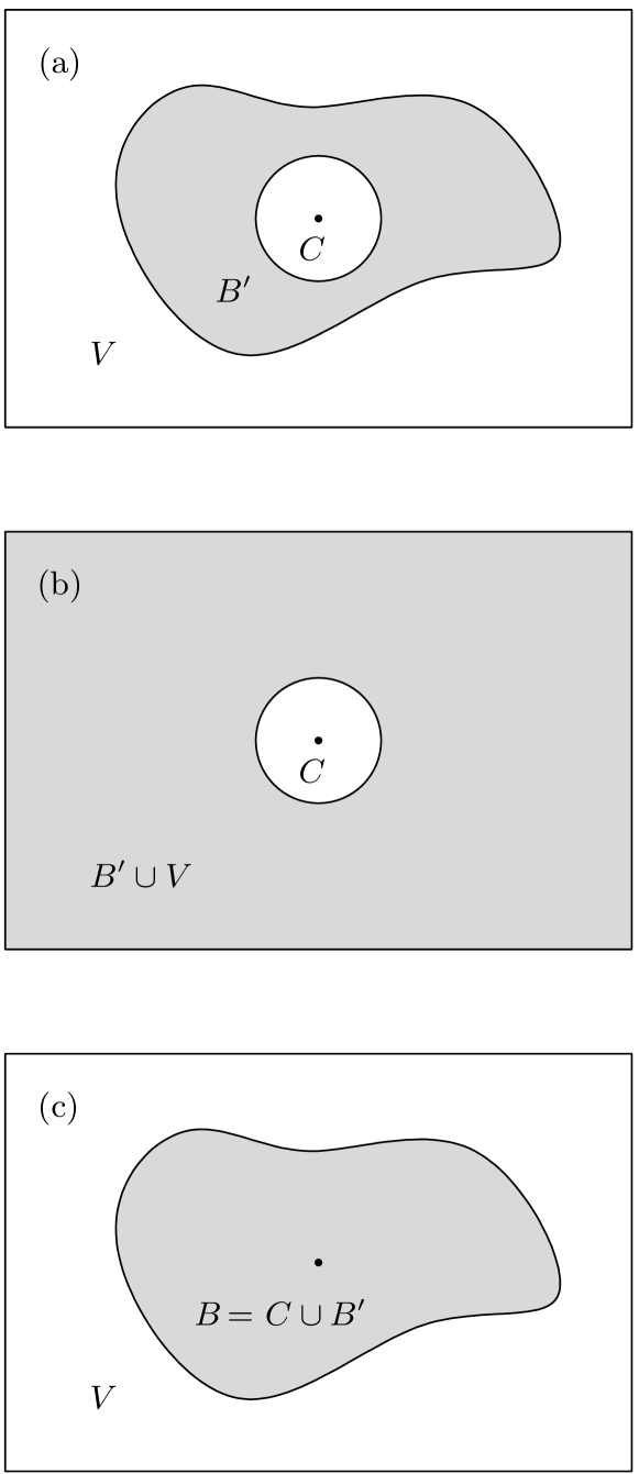
Figure 1: Schematic illustration of the decomposition of (a) $\bm{G}^{(1)}$ into (b) $\bm{G}^{(1)}_{\mathrm{C}}$ and (c) $\bm{G}_{\mathrm{B}}^{(1)}$; the dot indicates the position of the guest atom.

The cavity radius $R_{\mathrm{C}}$ is a model parameter representing an average distance from the atom to the nearest neighboring atoms constituting the host body; it has to be determined from other (preferably microscopic) calculations or experiments. Note that the real-cavity model is applicable provided that the unperturbed host body is homogeneous (and isotropic) in the region where the guest atom is implanted,

$$\varepsilon(\mathbf{r},\omega)=\varepsilon(\mathbf{r}_{\mathrm{A}},\omega)\quad\mbox{for }\mathbf{r}\in C.$$ (24)

III.1 Linear approximation

Restricting our attention to the first-order term in the Born expansion (20), the (scattering) Green tensor corresponding to $\varepsilon_{\mathrm{loc}}(\mathbf{r},\omega)$ can be calculated from Eq. (II.2), where after some manipulations one obtains

$$\bm{G}^{(1)}(\mathbf{r}_{\mathrm{A}},\mathbf{r}_{\mathrm{A}},\omega_{\mathrm{A}})=\frac{k_{\mathrm{A}}^{4}}{16\pi^{2}}\int_{B^{\prime}}\mathrm{d}^{3}s\,\chi(\mathbf{s},\omega_{\mathrm{A}})e^{(2i-\eta)q}$$

$$\hskip 86.11084pt\times[a^{2}\bm{I}+(b^{2}-2ab)\tilde{\mathbf{u}}\tilde{\mathbf{u}}]$$

$$\qquad=\bm{G}_{\mathrm{C}}^{(1)}(\mathbf{r}_{\mathrm{A}},\mathbf{r}_{\mathrm{A}},\omega_{\mathrm{A}})+\bm{G}_{\mathrm{B}}^{(1)}(\mathbf{r}_{\mathrm{A}},\mathbf{r}_{\mathrm{A}},\omega_{\mathrm{A}})$$ (25)

[$\mathbf{u}$ $\!=$ $\!\mathbf{r}_{\mathrm{A}}$ $\!-$ $\!\mathbf{s}$, $q$ $\!=$ $\!k_{\mathrm{A}}u$], where, again to linear order in the susceptibility,

$$\bm{G}_{\mathrm{C}}^{(1)}(\mathbf{r}_{\mathrm{A}},\mathbf{r}_{\mathrm{A}},\omega_{\mathrm{A}})=\frac{k_{\mathrm{A}}^{4}\chi(\omega_{\mathrm{A}})}{16\pi^{2}}\\ \times\int_{B^{\prime}\cup V}\mathrm{d}^{3}s\,e^{(2i-\eta)q}\bigl{[}a^{2}\bm{I}+(b^{2}-2ab)\tilde{\mathbf{u}}\tilde{\mathbf{u}}\bigr{]}$$ (26)

is the scattering Green tensor of a spherical cavity embedded in a bulk medium of susceptibility $\chi(\omega_{\mathrm{A}})$ $\!\equiv$ $\!\chi(\mathbf{r}_{\mathrm{A}},\omega_{\mathrm{A}})$ [cf. Fig. 1(b)], and

$$\bm{G}_{\mathrm{B}}^{(1)}(\mathbf{r}_{\mathrm{A}},\mathbf{r}_{\mathrm{A}},\omega_{\mathrm{A}})=\frac{k_{\mathrm{A}}^{4}}{16\pi^{2}}\int_{B}\mathrm{d}^{3}s\,\chi(\mathbf{s},\omega_{\mathrm{A}})e^{(2i-\eta)q}$$

$$\hskip 129.16626pt\times\bigl{[}a^{2}\bm{I}+(b^{2}-2ab)\tilde{\mathbf{u}}\tilde{\mathbf{u}}\bigr{]}$$

$$-\frac{k_{\mathrm{A}}^{4}\chi(\omega_{\mathrm{A}})}{16\pi^{2}}\int_{B\cup V}\mathrm{d}^{3}s\,e^{(2i-\eta)q}\bigl{[}a^{2}\bm{I}+(b^{2}-2ab)\tilde{\mathbf{u}}\tilde{\mathbf{u}}\bigr{]}$$ (27)

is the scattering part of the Green tensor of the host body without the cavity [cf. Fig. 1(c)]. The result can be verified by applying Eq. (5) [together with Eqs. (13) and (II.2)] to the two systems mentioned and using Eq. (24).

Equations (III.1)–(III.1) show that $\bm{G}^{(1)}$ in the rate formula (7) can be written as the sum of two terms, where the first term, $\bm{G}^{(1)}_{\mathrm{C}}$, only depends on the cavity radius and the local permittivity of the host body at the position of the atom, whereas the second term, $\bm{G}_{\mathrm{B}}^{(1)}$, is determined by the properties of the host body in the absence of the atom. Hence, the term in the decay rate which is proportional to $\mathrm{Im}\,\bm{G}^{(1)}_{\mathrm{C}}$ can be regarded as being the local-field correction to the uncorrected term proportional to $\mathrm{Im}\,\bm{G}^{(1)}_{\mathrm{B}}$. The fact that the local-field correction additively enters the rate formula is due to the linear expansion in $\chi$. Inspection of the second-order term in the Born expansion, Eq. (II.2), indicates that in general, terms depending on both the cavity and the (unperturbed) host body will appear which may lead to a breakdown of the additivity. However, as shown in Sec. III.2, there are situations where a generalization beyond the linear approximation is possible.

Equations (26) and (III.1) can be further evaluated by introducing a spherical coordinate system whose origin coincides with the position of the atom,

$$\int\mathrm{d}^{3}s\ \rightarrow\ \int_{0}^{2\pi}\mathrm{d}\phi\int_{0}^{\pi}\sin\theta\,\mathrm{d}\theta\int_{R_{\mathrm{i}}(\phi,\theta)}^{R_{\mathrm{o}}(\phi,\theta)}s^{2}\,\mathrm{d}s,$$ (28)

where $R_{\mathrm{i}}(\phi,\theta)$ and $R_{\mathrm{o}}(\phi,\theta)$, respectively, refer to the inner and outer boundary areas of the integration volumes sketched in Figs. 1(b) and 1(c). Performing the radial integral in Eq. (26), we find, on recalling Eq. (18),

$$\bm{G}^{(1)}_{\mathrm{C}}(\mathbf{r}_{\mathrm{A}},\mathbf{r}_{\mathrm{A}},\omega_{\mathrm{A}})=\lim_{\eta\to 0_{+}}\lim_{q\to\infty}\bm{F}_{\eta}(q)-\bm{F}_{0}(q_{\mathrm{C}})=-\bm{F}_{0}(q_{\mathrm{C}})$$ (29)

($q_{\mathrm{C}}$ $\!=$ $\!k_{\mathrm{A}}R_{\mathrm{C}}$) with

$$\bm{F}_{\eta}[q(\phi,\theta)]=-\frac{k_{\mathrm{A}}\chi(\omega_{\mathrm{A}})}{16\pi^{2}}\int_{0}^{2\pi}\mathrm{d}\phi\int_{0}^{\pi}\mathrm{d}\theta\sin\theta\biggl{\{}e^{(2i-\eta)q}$$

$$\times\biggl{[}\biggl{(}\frac{1}{3q^{3}}-\frac{2i}{3q^{2}}-\frac{5}{3q}+\frac{i}{2}\biggr{)}\bm{I}+\biggl{(}\frac{1}{q^{3}}-\frac{2i}{q^{2}}+\frac{3}{q}-\frac{i}{2}\biggr{)}\tilde{\mathbf{s}}\tilde{\mathbf{s}}\biggr{]}$$

$$\hskip 38.74988pt+4i\,\mathrm{Ei}[(2i\!-\!\eta)q]\biggl{(}\frac{1}{3}\bm{I}-\tilde{\mathbf{s}}\tilde{\mathbf{s}}\biggr{)}\biggr{\}}$$ (30)

[$q(\phi,\theta)$ $\!=$ $\!k_{\mathrm{A}}R(\phi,\theta)$; $\tilde{\mathbf{s}}$ $\!=$ $\!(\cos\phi\sin\theta,\sin\phi\sin\theta,\cos\theta)$; $\mathrm{Ei}(x)$, exponential integral]. Using the fact that $q_{\mathrm{C}}$ is independent of $\theta$ and $\phi$ as well as the relation

$$\int_{0}^{2\pi}\mathrm{d}\phi\int_{0}^{\pi}\mathrm{d}\theta\,\sin\theta\,\tilde{\mathbf{s}}\tilde{\mathbf{s}}=\frac{4\pi}{3}\bm{I},$$ (31)

from Eq. (III.1) we obtain

$$\bm{F}_{0}(q_{\mathrm{C}})=-\frac{k_{\mathrm{A}}\chi(\omega_{\mathrm{A}})}{12\pi}\biggl{(}\frac{2}{q_{\mathrm{C}}^{3}}-\frac{4i}{q_{\mathrm{C}}^{2}}-\frac{2}{q_{\mathrm{C}}}+i\biggr{)}e^{2iq_{\mathrm{C}}}\bm{I}.$$ (32)

In particular, when the radius of the cavity is much smaller than the atomic transition wavelength,

$$q_{\mathrm{C}}=k_{\mathrm{A}}R_{\mathrm{C}}\ll 1,$$ (33)

then Eq. (32) reduces to

$$\bm{F}_{0}(q_{\mathrm{C}})=-\frac{k_{\mathrm{A}}\chi(\omega_{\mathrm{A}})}{6\pi}\biggl{[}\frac{1}{q_{\mathrm{C}}^{3}}+\frac{1}{q_{\mathrm{C}}}+\frac{7i}{6}+O(q_{\mathrm{C}})\biggr{]}\bm{I}.$$ (34)

Substitution of this result together with Eq. (29) into Eq. (III.1) reveals that to linear order in $\chi$,

$$\bm{G}^{(1)}(\mathbf{r}_{\mathrm{A}},\mathbf{r}_{\mathrm{A}},\omega_{\mathrm{A}})=\frac{k_{\mathrm{A}}\chi(\omega_{\mathrm{A}})}{6\pi}\biggl{[}\frac{1}{(k_{\!\mathrm{A}}\!R_{\mathrm{C}})^{3}}+\frac{1}{k_{\!\mathrm{A}}\!R_{\mathrm{C}}}+\frac{7i}{6}\biggr{]}\bm{I}\\ +\bm{G}_{\mathrm{B}}^{(1)}(\mathbf{r}_{\mathrm{A}},\mathbf{r}_{\mathrm{A}},\omega_{\mathrm{A}})+O(k_{\mathrm{A}}R_{\mathrm{C}}).$$ (35)

For a homogeneous host body which is star-shaped w.r.t. the position of the atom (i.e., every point on the outer boundary area can be connected to the atomic position by a straight line that lies entirely within the body), $\bm{G}_{\mathrm{B}}^{(1)}$ as given by Eq. (III.1) can be evaluated in a similar manner. Using again spherical coordinates and recalling Eq. (18), we may evaluate the radial integrals in Eq. (III.1) to obtain

$$\bm{G}_{\mathrm{B}}^{(1)}(\mathbf{r}_{\mathrm{A}},\mathbf{r}_{\mathrm{A}},\omega_{\mathrm{A}})=\lim_{\eta\to 0_{+}}\bm{F}_{\eta}[q_{\mathrm{o}}(\phi,\theta)]-\bm{F}_{0}(0)$$

$$\quad-\Bigl{[}\lim_{\eta\to 0_{+}}\lim_{q\to\infty}\bm{F}_{\eta}(q)-\bm{F}_{0}(0)\Bigr{]}=\lim_{\eta\to 0_{+}}\bm{F}_{\eta}[q_{\mathrm{o}}(\phi,\theta)]$$ (36)

[$q_{\mathrm{o}}$ $\!=$ $\!q_{\mathrm{o}}(\phi,\theta)$ $\!=$ $\!k_{\mathrm{A}}R_{\mathrm{o}}(\phi,\theta)$], where henceforth $R_{\mathrm{o}}(\phi,\theta)$ denotes the outer boundaries of the host body.

Substituting Eq. (35) into Eq. (7), we find that to linear order in $\chi$ the local-field corrected spontaneous-decay rate of an atom within a body can be given as follows:

$$\Gamma=\Gamma_{0}+\Gamma_{\mathrm{C}}+\Gamma_{\mathrm{B}}^{(1)},$$ (37)

where $\Gamma_{0}$ is the free-space decay rate as given in Eq. (8),

$$\frac{\Gamma_{\mathrm{C}}}{\Gamma_{0}}=\frac{\mathrm{Im}\,\chi(\omega_{\mathrm{A}})}{(k_{\mathrm{A}}R_{\mathrm{C}})^{3}}+\frac{\mathrm{Im}\,\chi(\omega_{\mathrm{A}})}{k_{\mathrm{A}}R_{\mathrm{C}}}+\frac{7\,\mathrm{Re}\,\chi(\omega_{\mathrm{A}})}{6},$$ (38)

and

$$\Gamma^{(1)}_{\mathrm{B}}=\frac{2k_{\mathrm{A}}^{2}}{\hbar\varepsilon_{0}}\,\mathbf{d}_{\mathrm{A}}\!\cdot\!\mathrm{Im}\,\bm{G}_{\mathrm{B}}^{(1)}(\mathbf{r}_{\mathrm{A}},\mathbf{r}_{\mathrm{A}},\omega_{\mathrm{A}})\!\cdot\!\mathbf{d}_{\mathrm{A}}.$$ (39)

Equations (37)–(39) are valid for an atom embedded in a weakly polarizable, dispersing and absorbing body of arbitrary size and shape. Note that only $\Gamma_{\mathrm{C}}$ takes into account the effect of local-field correction, while $\Gamma_{\mathrm{B}}^{(1)}$, which is simply determined by the scattering part of the Green tensor of the host body without the cavity, reflects the uncorrected influence of the size and shape of the body on the decay rate. In particular, the first two terms in Eq. (38) obviously result from irreversible energy transfer from the atom to the surrounding matter. If these two terms are dominant over the last one, effectively no radiation is emitted.

We conclude this section by making two remarks concerning the necessary conditions under which Eq. (37) provides a good approximation to the spontaneous-decay rate. (i) The permittivity often appears in the Green tensor as a common factor $\sqrt{\varepsilon}\omega R_{\mathrm{o}}/c$ [cf. Eq. (82) in Sec. IV.2.1]. To be on the conservative side, one should then take $\chi k_{\mathrm{A}}R_{\mathrm{max}}$ [with $R_{\mathrm{max}}$ $\!=$ $\max_{(\theta,\phi)}R_{\mathrm{o}}(\theta,\phi)$] rather than $\chi$ as the small parameter. (ii) Equation (38) already contains terms of the order of $\mathrm{Im}\,\chi/(k_{\mathrm{A}}R_{\mathrm{C}})^{3}$. Thus $\mathrm{Im}\,\chi/(k_{\mathrm{A}}R_{\mathrm{C}})^{3}$, not $\mathrm{Im}\,\chi$, should be much smaller than unity for the linear approximation to yield a good estimation of the decay rate. The cavity radius $R_{\mathrm{C}}$ represents the average distance between the atom and the constituents of the body. For, say, $k_{\mathrm{A}}R_{\mathrm{C}}$ $\!\gtrsim$ $\!0.01$, it is sufficient to require that $\mathrm{Im}\,\chi$ $\!\ll$ $\!10^{-6}$, so that $\mathrm{Im}\,\chi/(k_{\mathrm{A}}R_{\mathrm{C}})^{3}$ $\!\ll$ $\!1$.

III.2 Beyond the linear approximation

Tomaš Tomas01 has found that in the special case of an atom situated at the center of a homogenous, dielectric sphere, the real-cavity model (Fig. 2 in the case where $l_{\mathrm{A}}$ $\!=$ $\!0$) leads to

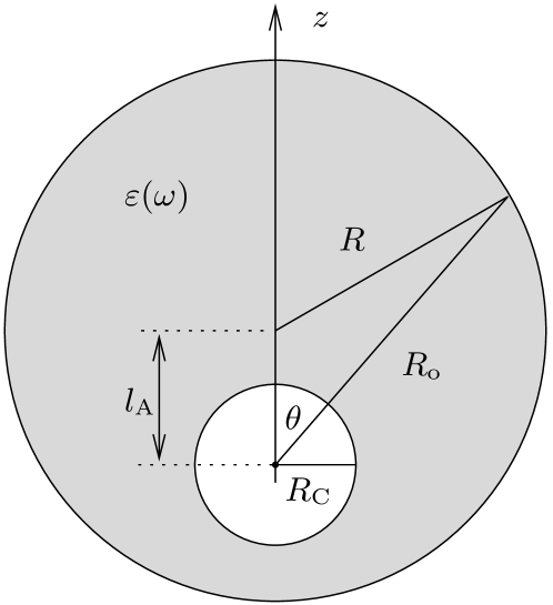
Figure 2: Real-cavity model for an atom embedded in a homogeneous dielectric sphere.

the relation

$$\bm{G}^{(1)}(\mathbf{r}_{\mathrm{A}},\mathbf{r}_{\mathrm{A}},\omega_{\mathrm{A}})=\frac{k_{\mathrm{A}}}{6\pi}\biggl{\{}\frac{3(\varepsilon-1)}{2\varepsilon+1}\,\frac{1}{(k_{\mathrm{A}}R_{\mathrm{C}})^{3}}$$

$$\quad+\frac{9(\varepsilon-1)(4\varepsilon+1)}{5(2\varepsilon+1)^{2}}\,\frac{1}{k_{\mathrm{A}}R_{\mathrm{C}}}+i\biggl{[}\frac{9\varepsilon^{5/2}}{(2\varepsilon+1)^{2}}-1\biggr{]}\biggr{\}}\bm{I}$$

$$\quad+\biggl{(}\frac{3\varepsilon}{2\varepsilon+1}\biggr{)}^{2}\bm{G}_{\mathrm{B}}^{(1)}(\mathbf{r}_{\mathrm{A}},\mathbf{r}_{\mathrm{A}},\omega_{\mathrm{A}})+O(k_{\mathrm{A}}R_{\mathrm{C}}),$$ (40)

$\varepsilon$ $\!=$ $\varepsilon(\omega_{\mathrm{A}})$, where $\bm{G}_{\mathrm{B}}^{(1)}(\mathbf{r},\mathbf{r}^{\prime},\omega)$ is the scattering Green tensor of the homogeneous dielectric sphere, whose geometry dependence is—for $\mathbf{r}$ $\!=$ $\!\mathbf{r}^{\prime}$ $\!=$ $\!\mathbf{r}_{\mathrm{A}}$ at the sphere center—entirely given by its dependence on the sphere radius $R$. As already mentioned in Sec. I, he made the conjecture that this relation might be more generally valid for (i) bodies of arbitrary sizes and shapes and (ii) arbitrary positions of the atom, provided that the atom is not on the body surface.

Let us study the validity of this conjecture in more detail. It can easily be seen that to linear order in $\chi$, Eq. (III.2) obviously reduces to Eq. (35), so the results of Sec. III.1 show that in this order the conjecture is true even under the more general conditions of inhomogeneous host bodies, provided that the requirement (24) for the applicability of the real-cavity model is valid. Moreover, we will demonstrate in the following that Eq. (III.2) remains valid beyond the linear order in $\chi$, provided that the respective host body can be regarded as being homogeneous in the vicinity of the atom, i.e.,

$$\varepsilon(\mathbf{r},\omega_{\mathrm{A}})=\varepsilon(\mathbf{r}_{\mathrm{A}},\omega_{\mathrm{A}})\quad\mbox{for }|\mathbf{r}-\mathbf{r}_{\mathrm{A}}|\leq(1+\nu)R_{\mathrm{C}},$$ (41)

with $\nu$ being some small positive number.

We begin with the case of a homogeneous body, in which case satisfaction of the condition (41) simply ensures that the entire cavity lies inside the body. We first recall that $\bm{G}^{(1)}(\mathbf{r}_{\mathrm{A}},\mathbf{r}_{\mathrm{A}},\omega_{\mathrm{A}})$ determines the electric field reaching the point $\mathbf{r}_{\mathrm{A}}$, in which it has originated, after being scattered at the surfaces of inhomogeneity [cf. Fig. 1(a)]. At the cavity surface the electric field can be separated into two parts, namely, one part that is (multiply) reflected at this surface and eventually returns to the point $\mathbf{r}_{\mathrm{A}}$, and one part that is eventually transmitted to the exterior of the cavity. The contribution due to the reflected part is obviously given by $\bm{G}^{(1)}_{\mathrm{C}}(\mathbf{r}_{\mathrm{A}},\mathbf{r}_{\mathrm{A}},\omega_{\mathrm{A}})$ [cf. Fig. 1(b)], which reads Scheel99b ; Tomas01

$$\bm{G}^{(1)}_{\mathrm{C}}(\mathbf{r}_{\mathrm{A}},\mathbf{r}_{\mathrm{A}},\omega_{\mathrm{A}})=\frac{k_{\mathrm{A}}}{6\pi}\biggl{\{}\frac{3(\varepsilon-1)}{2\varepsilon+1}\,\frac{1}{(k_{\mathrm{A}}R_{\mathrm{C}})^{3}}$$

$$\quad+\frac{9(\varepsilon-1)(4\varepsilon+1)}{5(2\varepsilon+1)^{2}}\,\frac{1}{k_{\mathrm{A}}R_{\mathrm{C}}}+i\biggl{[}\frac{9\varepsilon^{5/2}}{(2\varepsilon+1)^{2}}-1\biggr{]}\biggr{\}}\bm{I}$$

$$\quad+O(k_{\mathrm{A}}R_{\mathrm{C}}).$$ (42)

In an infinitely extended body [cf. Fig. 1(b)], the transmitted part at a point $\mathbf{r}$ outside the cavity is determined by the Green tensor Li94

$$\bm{G}_{\mathrm{C}}(\mathbf{r},\mathbf{r}_{\mathrm{A}},\omega_{\mathrm{A}})=\frac{k_{\mathrm{A}}A}{4\pi}\,(a\bm{I}-b\tilde{\mathbf{u}}\tilde{\mathbf{u}})e^{iq}$$ (43)

[$\mathbf{u}$ $\!=$ $\!\mathbf{r}$ $\!-$ $\!\mathbf{r}_{\mathrm{A}}$, $q$ $\!=$ $\!nk_{\mathrm{A}}u$, $n$ $\!=$ $\sqrt{\varepsilon}$, and $a$ and $b$ according to Eq. (18)]. The coefficient $A$ (which corresponds to $A_{N}^{12}$ in Ref. Li94 ) is given by

$$A=n\,\frac{j_{1}(z_{0})[z_{0}h_{1}^{(1)}(z_{0})]^{\prime}-[z_{0}j_{1}(z_{0})]^{\prime}h_{1}^{(1)}(z_{0})}{j_{1}(z_{0})[z_{1}h_{1}^{(1)}(z_{1})]^{\prime}-\varepsilon[z_{0}j_{1}(z_{0})]^{\prime}h_{1}^{(1)}(z_{1})}\,,$$ (44)

where $z_{0}$ $\!=$ $\!k_{\mathrm{A}}R_{\mathrm{C}}$, $z_{1}$ $\!=$ $\!nk_{\mathrm{A}}R_{\mathrm{C}}$ (the primes denote derivatives w.r.t. $z_{0}$ and $z_{1}$), and

$$j_{1}(z)=\frac{\sin z}{z^{2}}-\frac{\cos z}{z}$$ (45)

and

$$h_{1}^{(1)}(z)=-\biggl{(}\frac{1}{z}+\frac{i}{z^{2}}\biggr{)}e^{iz}$$ (46)

are the spherical Bessel and Hankel functions, respectively. Inspection of Eq. (44) shows that

$$A=n\,\frac{3\varepsilon}{2\varepsilon+1}+O(k_{\mathrm{A}}R_{\mathrm{C}}).$$ (47)

Substitution of this result into Eq. (43) leads to

$$\bm{G}_{\mathrm{C}}(\mathbf{r},\mathbf{r}_{\mathrm{A}},\omega_{\mathrm{A}})=\frac{3\varepsilon}{2\varepsilon+1}\,\bm{G}_{\mathrm{B}}^{(0)}(\mathbf{r},\mathbf{r}_{\mathrm{A}},\omega_{\mathrm{A}})+O(k_{\mathrm{A}}R_{C}),$$ (48)

where $\bm{G}_{\mathrm{B}}^{(0)}(\mathbf{r},\mathbf{r}_{\mathrm{A}},\omega_{\mathrm{A}})$ is the Green tensor of the infinite body without the cavity [according to Eqs. (17) and (18) with $k\mapsto nk$]. In other words, the electric field transmitted through the cavity surface to a point outside the cavity is equal to the field that would be transmitted to the same point in the absence of the cavity, multiplied by a global factor. By means of the general symmetry property (see, e.g., Ref. Knoell01 )

$$\bm{G}(\mathbf{r},\mathbf{r}^{\prime},\omega)=\bm{G}^{\mathrm{T}}(\mathbf{r}^{\prime},\mathbf{r},\omega)$$ (49)

we also have

$$\bm{G}_{\mathrm{C}}(\mathbf{r}_{\mathrm{A}},\mathbf{r},\omega_{\mathrm{A}})=\frac{3\varepsilon}{2\varepsilon+1}\,\bm{G}_{\mathrm{B}}^{(0)}(\mathbf{r}_{\mathrm{A}},\mathbf{r},\omega_{\mathrm{A}})+O(k_{\mathrm{A}}R_{\mathrm{C}}),$$ (50)

i.e., the electric field transmitted through the cavity surface from an arbitrary point outside the cavity is also equal to the corresponding result in the absence of the cavity, multiplied by the same factor.

For a finite body, the electric field will be (multiply) reflected from the body’s outer surface, eventually giving rise to a field at $\mathbf{r}_{\mathrm{A}}$. Without the cavity, processes of this kind are taken into account by replacing the infinite-body Green tensor $\bm{G}_{\mathrm{B}}^{(0)}$ with its finite-body counterpart $\!\bm{G}_{\mathrm{B}}$. Combining this observation with Eqs. (48) and (50), we conclude, on recalling the linearity of Maxwell’s equations, that the electric field which is transmitted though the cavity surface, scattered at the outer body surface, and finally retransmitted into the cavity is given by

$$\biggl{(}\frac{3\varepsilon}{2\varepsilon+1}\biggr{)}^{2}\,\bm{G}_{\mathrm{B}}^{(1)}(\mathbf{r}_{\mathrm{A}},\mathbf{r}_{\mathrm{A}},\omega_{A})+O(k_{\mathrm{A}}R_{\mathrm{C}}),$$ (51)

so combining Eqs. (III.2) and (51), we arrive at Eq. (III.2).

In this derivation, we have disregarded processes involving scattering of the field at the cavity surface from the outside. Processes of this kind can indeed be neglected, because their contributions are of orders higher than $O(k_{\mathrm{A}}R_{\mathrm{C}})$. To see this, note that for a cavity in bulk material [Fig. 1(b)] the field at a point $\mathbf{r}$ outside the cavity originating in a point $\mathbf{r}^{\prime}$ outside the cavity via scattering at the cavity surface, is characterized by Li94

$$\bm{G}^{(1)}_{\mathrm{C}}(\mathbf{r},\mathbf{r}^{\prime},\omega_{\mathrm{A}})\\ =\sum_{m=1}^{\infty}\Big{[}B_{m}^{M}\bm{M}(\mathbf{r},\mathbf{r}^{\prime},\omega_{\mathrm{A}})+B_{m}^{N}\bm{N}(\mathbf{r},\mathbf{r}^{\prime},\omega_{\mathrm{A}})\Big{]},$$ (52)

where

$$B_{m}^{M}=-\frac{j_{m}(z_{0})[z_{1}j_{m}(z_{1})]^{\prime}-[z_{0}j_{m}(z_{0})]^{\prime}j_{m}(z_{1})}{j_{m}(z_{0})[z_{1}h_{m}^{(1)}(z_{1})]^{\prime}-[z_{0}j_{m}(z_{0})]^{\prime}h_{m}^{(1)}(z_{1})}\,,$$ (53)

$$B_{m}^{N}=-\frac{j_{m}(z_{0})[z_{1}j_{m}(z_{1})]^{\prime}-\varepsilon[z_{0}j_{m}(z_{0})]^{\prime}j_{m}(z_{1})}{j_{m}(z_{0})[z_{1}h_{m}^{(1)}(z_{1})]^{\prime}-\varepsilon[z_{0}j_{m}(z_{0})]^{\prime}h_{m}^{(1)}(z_{1})},$$ (54)

and the tensors $\bm{M}(\mathbf{r},\mathbf{r}^{\prime},\omega_{\mathrm{A}})$ and $\bm{N}(\mathbf{r},\mathbf{r}^{\prime},\omega_{\mathrm{A}})$ do not depend on $R_{\mathrm{C}}$. Using the relations Abramowitz73

$$j_{m}(z)=\frac{z^{m}}{(2m+1)!!}\bigl{[}1+O(z^{2})\bigr{]},$$ (55)

$$h_{m}^{(1)}(z)=-\frac{i(2m-1)!!}{z^{m+1}}\bigl{[}1+O(z^{2})\bigr{]},$$ (56)

one can easily show that

$$B_{m}^{M}=O\bigl{[}(k_{\mathrm{A}}R_{\mathrm{C}})^{2m+3}\bigr{]},\quad B_{m}^{N}=O\bigl{[}(k_{\mathrm{A}}R_{\mathrm{C}})^{2m+1}\bigr{]},$$ (57)

so Eq. (52) leads to

$$\bm{G}^{\mathrm{(1)}}_{\mathrm{C}}(\mathbf{r},\mathbf{r}^{\prime},\omega_{\mathrm{A}})=O\bigl{[}(k_{\mathrm{A}}R_{\mathrm{C}})^{3}\bigr{]}.$$ (58)

Processes involving reflections of the field at the cavity surface from the outside hence start to contribute in third order of $k_{\mathrm{A}}R_{\mathrm{C}}$ and therefore do not need to be included in Eq. (III.2).

So far we have demonstrated the validity of the relation (III.2) for homogeneous dielectric bodies of arbitrary shapes provided that the atom is situated at the interior of the body, such that the condition (41) is satisfied. Note that this condition practically coincides with the condition (24) for the applicability of the real-cavity model. The arguments given above can be extended to inhomogeneous bodies. If the condition (41) is satisfied, one can divide such a body into a more or less small homogeneous part containing the cavity plus an inhomogeneous rest. Equations (48), (50), and (58) then still describe the propagation of the electric field inside the homogeneous part of the body, and the effect of the inhomogeneous part can be taken into account by the scattering at the (fictitious) surface dividing the two parts. Consequently, we are again left with Eq. (III.2).

Substituting Eq. (III.2) into Eq. (7) and recalling Eq. (8), we can again cast the local-field corrected spontaneous-decay rate in the form of of Eq. (37), where now

$$\frac{\Gamma_{\mathrm{C}}}{\Gamma_{0}}= \;\mathrm{Im}\biggl{\{}\frac{3(\varepsilon-1)}{2\varepsilon+1}\,\frac{1}{(k_{\mathrm{A}}R_{\mathrm{C}})^{3}}+\frac{9(\varepsilon-1)(4\varepsilon+1)}{5(2\varepsilon+1)^{2}}\,\frac{1}{k_{\mathrm{A}}R_{\mathrm{C}}}$$

$$\;+i\biggl{[}\frac{9\varepsilon^{5/2}}{(2\varepsilon+1)^{2}}-1\biggr{]}\biggr{\}},$$ (59)

and

$$\Gamma_{\mathrm{B}}^{(1)}=\frac{2k_{\mathrm{A}}^{2}}{\hbar\varepsilon_{0}}\,\mathbf{d}_{\mathrm{A}}\!\cdot\!\mathrm{Im}\biggl{[}\biggl{(}\frac{3\varepsilon}{2\varepsilon+1}\biggr{)}^{2}\bm{G}_{\mathrm{B}}^{(1)}(\mathbf{r}_{\mathrm{A}},\mathbf{r}_{\mathrm{A}},\omega_{\mathrm{A}})\biggr{]}\!\cdot\mathbf{d}_{\mathrm{A}}$$ (60)

[$\varepsilon$ $\!=$ $\varepsilon(\mathbf{r}_{\mathrm{A}},\omega_{\mathrm{A}})$]. Recall that $\bm{G}_{\mathrm{B}}^{(1)}$ is the (unperturbed) scattering part of the Green tensor of the host body without the cavity. Needless to say that to linear order in $\chi$, Eqs. (III.2) and (60) reduce to Eqs. (38) and (39), respectively.

In particular in the case of weakly absorbing matter, it may be sufficient to retain in Eqs. (III.2) and (60) only terms to linear order in $\mathrm{Im}\,\varepsilon$. From Eqs. (37), (III.2), and (60) it then follows that when

$$\left|\frac{\mathrm{Im}\,\varepsilon\,\mathbf{d}_{\mathrm{A}}\cdot\mathrm{Re}\,\bm{G}_{\mathrm{B}}^{(1)}(\mathbf{r}_{\mathrm{A}},\mathbf{r}_{\mathrm{A}},\omega_{\mathrm{A}})\cdot\mathbf{d}_{\mathrm{A}}}{\mathrm{Re}\,\varepsilon\,\mathbf{d}_{\mathrm{A}}\cdot\mathrm{Im}\,\bm{G}_{\mathrm{B}}(\mathbf{r}_{\mathrm{A}},\mathbf{r}_{\mathrm{A}},\omega_{\mathrm{A}})\cdot\mathbf{d}_{\mathrm{A}}}\right|\ll 1$$ (61)

then $\Gamma$ can be given in the form

$$\Gamma=\left(\frac{3\,\mathrm{Re}\,\varepsilon}{2\,\mathrm{Re}\,\varepsilon+1}\right)^{2}\Gamma_{\mathrm{B}}+\Delta\Gamma,$$ (62)

where

$$\frac{\Delta\Gamma}{\Gamma_{0}}= \,\frac{9}{(2\,\mathrm{Re}\,\varepsilon+1)^{2}}\,\frac{\mathrm{Im}\,\varepsilon}{(k_{\mathrm{A}}R_{\mathrm{C}})^{3}}$$

$$+\frac{9(14\mathrm{Re}\,\varepsilon+1)}{5(2\,\mathrm{Re}\,\varepsilon+1)^{3}}\,\frac{\mathrm{Im}\,\varepsilon}{k_{\mathrm{A}}R_{\mathrm{C}}}\,,$$ (63)

and $\Gamma_{\mathrm{B}}$ is the uncorrected decay rate as given by Eq. (10) with $\bm{G}^{(1)}(\mathbf{r}_{\mathrm{A}},\mathbf{r}_{\mathrm{A}},\omega_{\mathrm{A}})$ $\!\equiv$ $\bm{G}_{\mathrm{B}}^{(1)}(\mathbf{r}_{\mathrm{A}},\mathbf{r}_{\mathrm{A}},\omega_{\mathrm{A}})$. Rahmani and Bryant Rahmani02 concluded from a numerical computation of the Green tensor of a dielectric sphere that contains a (small) empty sphere at an arbitrary position inside the material that the local-field corrected spontaneous decay rate has the form $\Gamma$ $\!=$ $f^{2}\Gamma_{\mathrm{B}}$ $\!+$ $\delta\Gamma$, where the shift term $\delta\Gamma$ is due to absorption. Comparing with Eq. (62) [together with Eq. (III.2)], we see that this is indeed the case when the effect of absorption is sufficiently weak and in particular, the inequality (61) holds. However, from Eqs. (37), (III.2), and (60) it is clearly seen that in general, $\Gamma$ cannot be given in the form assumed in Ref. Rahmani02 . Note that already the analytical solution for the special case considered in Ref. Tomas01 implies that this form cannot be true in general.

IV Examples

IV.1 Atom in a bulk medium

In the case of bulk material, we have $\bm{G}_{\mathrm{B}}^{(1)}$ $\!=$ $\!0$, so Eq. (37) simplifies to

$$\Gamma=\Gamma_{0}+\Gamma_{\mathrm{C}},$$ (64)

where $\Gamma_{\mathrm{C}}/\Gamma_{0}$ is given by Eq. (III.2) Scheel99b ; Tomas01 , which to linear order in $\chi$ reduces to Eq. (38). In particular, when material absorption can be neglected, $\varepsilon$ $\!\simeq$ $\!\mathrm{Re}\,\varepsilon$, we simply have Glauber91

$$\Gamma=\biggl{(}\frac{3\varepsilon}{2\varepsilon+1}\biggr{)}^{2}\sqrt{\varepsilon}\,\Gamma_{0}$$ (65)

[which follows directly from Eq. (62) with $\Gamma_{\mathrm{B}}$ $\!=$ $\!\sqrt{\varepsilon}\Gamma_{0}$, cf. Eq. (10)]. Note that in this case the virtual-cavity model leads to

$$\Gamma=\biggl{(}\frac{\varepsilon+2}{3}\biggr{)}^{2}\sqrt{\varepsilon}\,\Gamma_{0}$$ (66)

(see, e.g., Ref. Scheel99a ). It is not difficult to see that to linear order in $\chi$ both Eq. (65) and Eq. (66) lead to

$$\Gamma=\biggl{[}1+\frac{7\chi(\omega_{\mathrm{A}})}{6}\biggr{]}\Gamma_{0},$$ (67)

i.e., the first-order theory for the spontaneous decay rate does not distinguish between the virtual- and the real-cavity model Berman04 , provided that absorption can be disregarded.

IV.2 Atom in a sphere

Let us consider an atom in a homogeneous dielectric sphere as sketched in Fig. 2 and first calculate the spontaneous-decay rate to linear order in $\chi$. In particular, we need to calculate $\Gamma_{\mathrm{B}}^{(1)}$ as given by Eq. (39) with $\bm{G}_{\mathrm{B}}^{(1)}$ from Eq. (III.1) together with Eq. (III.1). Noting that

$$q_{\mathrm{o}}(\phi,\theta)=k_{\mathrm{A}}\Bigl{[}l_{\mathrm{A}}\cos\theta+\sqrt{R^{2}-l_{\mathrm{A}}^{2}(1-\cos^{2}\theta)}\Bigl{]}$$ (68)

(cf. Fig. 2) is independent of $\phi$, performing the $\phi$-integral, and using the fact that $\mathbf{d}_{\mathrm{A}}\cdot\tilde{\mathbf{s}}$ $\!=$ $\!d_{\mathrm{A}}\cos\theta$ for a radially ($\perp$) oriented dipole and $\mathbf{d}_{\mathrm{A}}\cdot\tilde{\mathbf{s}}$ $\!=$ $\!d_{\mathrm{A}}\sin\theta\cos\phi$ for a tangentially ($\parallel$) oriented dipole, we find

$$\Gamma_{\mathrm{B}}^{(1)\perp(\parallel)}=-\frac{3\Gamma_{0}}{4}\,\lim_{\eta\to 0}\mathrm{Im}\biggl{[}\chi(\omega_{\mathrm{A}})\int_{-1}^{1}\mathrm{d}x\,f_{\eta}^{\perp(\parallel)}(q_{\mathrm{o}},x^{2})\biggr{]},$$ (69)

where

$$f_{\eta}^{\perp}(q_{\mathrm{o}},z)= \;\biggl{[}\frac{1}{3q_{\mathrm{o}}^{3}}-\frac{2i}{3q_{\mathrm{o}}^{2}}-\frac{5}{3q_{\mathrm{o}}}+\frac{i}{2}$$

$$\quad+\biggl{(}\frac{1}{q_{\mathrm{o}}^{3}}-\frac{2i}{q_{\mathrm{o}}^{2}}+\frac{3}{q_{\mathrm{o}}}-\frac{i}{2}\biggr{)}z\biggr{]}e^{(2i-\eta)q_{\mathrm{o}}}$$

$$+4i\biggl{(}\frac{1}{3}-z\biggr{)}\mathrm{Ei}[(2i-\eta)q_{\mathrm{o}}],$$ (70)

$$f_{\eta}^{\parallel}(q_{\mathrm{o}},z)= \;f_{\eta}^{\perp}[q_{\mathrm{o}},(1-z)/2],$$ (71)

and $q_{\mathrm{o}}$ according to Eq. (68), with $\cos\theta$ being replaced by $x$.

In order to exactly calculate $\Gamma_{\mathrm{B}}^{(1)}$ [Eq. (60)], we make use of the exact Green tensor for a dielectric sphere as given in Ref. Li94 , leading to

$$\Gamma_{\mathrm{B}}^{(1)\perp}=\frac{3\Gamma_{0}}{2}\,\mathrm{Im}\biggl{\{}\frac{9i\varepsilon^{5/2}}{(2\varepsilon+1)^{2}}\sum_{m=1}^{\infty}(2m+1)\\ \times m(m+1)C^{N}_{m}\biggl{[}\frac{j_{m}(nk_{\mathrm{A}}l_{\mathrm{A}})}{nk_{\mathrm{A}}l_{\mathrm{A}}}\biggr{]}^{2}\biggr{\}},$$ (72)

$$\Gamma_{\mathrm{B}}^{(1)\|}=\frac{3\Gamma_{0}}{4}\,\mathrm{Im}\biggl{\{}\frac{9i\varepsilon^{5/2}}{(2\varepsilon+1)^{2}}\sum_{m=1}^{\infty}(2m+1)\\ \times\biggl{[}C^{M}_{m}j_{m}^{2}(nk_{\mathrm{A}}l_{\mathrm{A}})+C^{N}_{m}\biggl{(}\frac{\mathrm{d}[l_{\mathrm{A}}j_{m}(nk_{\mathrm{A}}l_{\mathrm{A}})]}{(nk_{\mathrm{A}}l_{\mathrm{A}})\mathrm{d}l_{\mathrm{A}}}\biggr{)}^{2}\biggr{]}\biggr{\}},$$ (73)

where

$$C^{N}_{m}=-\frac{\varepsilon h_{m}^{(1)}(z_{1})[z_{0}h_{m}^{(1)}(z_{0})]^{\prime}-[z_{1}h_{m}^{(1)}(z_{1})]^{\prime}h_{m}^{(1)}(z_{0})}{\varepsilon j_{m}^{(1)}(z_{1})[z_{0}h_{m}^{(1)}(z_{0})]^{\prime}-[z_{1}j_{m}^{(1)}(z_{1})]^{\prime}h_{m}^{(1)}(z_{0})}\,,$$ (74)

$$C^{M}_{m}=-\frac{h_{m}^{(1)}(z_{1})[z_{0}h_{m}^{(1)}(z_{0})]^{\prime}-[z_{1}h_{m}^{(1)}(z_{1})]^{\prime}h_{m}^{(1)}(z_{0})}{j_{m}^{(1)}(z_{1})[z_{0}h_{m}^{(1)}(z_{0})]^{\prime}-[z_{1}j_{m}^{(1)}(z_{1})]^{\prime}h_{m}^{(1)}(z_{0})}\,,$$ (75)

with $z_{0}$ $\!\equiv$ $\!k_{\mathrm{A}}R$, $z_{1}$ $\!\equiv$ $\!nk_{\mathrm{A}}R$.

IV.2.1 Atom on center

To compare the exact decay rate [Eq. (37) together with Eqs. (8), and (III.2) as well as Eqs. (72) and/or (73)] with the decay rate obtained in the linear Born approximation [Eq. (37) together with Eqs. (8), (38), and (69)], let us consider, for simplicity, the case where the atom is positioned at the center of the sphere. Setting $l_{\mathrm{A}}$ $\!=$ $\!0$ and hence, $q_{\mathrm{o}}$ $\!=$ $\!k_{\mathrm{A}}R$ in Eqs. (69)–(71), and carrying out the $x$ integral in Eq. (69), we derive

$$\Gamma_{\mathrm{B}}^{(1)\perp}=\Gamma_{\mathrm{B}}^{(1)\parallel}=\Gamma_{\mathrm{B}}^{(1)}$$ (76)

with

$$\Gamma_{\mathrm{B}}^{(1)}=-\Gamma_{0}\lim_{\eta\to 0}\mathrm{Im}\biggl{\{}\chi(\omega_{\mathrm{A}})\biggl{[}\frac{1}{(k_{\mathrm{A}}R)^{3}}-\frac{2i}{(k_{\mathrm{A}}R)^{2}}\\ -\frac{1}{k_{\mathrm{A}}R}+\frac{i}{2}\biggr{]}e^{(2i-\eta)k_{\mathrm{A}}R}\biggr{\}},$$ (77)

giving

$$\Gamma_{\mathrm{B}}^{(1)}=-\Gamma_{0}\mathrm{Im}\biggl{\{}\chi(\omega_{\mathrm{A}})\biggl{[}\frac{1}{(k_{\mathrm{A}}R)^{3}}-\frac{2i}{(k_{\mathrm{A}}R)^{2}}\\ -\frac{1}{k_{\mathrm{A}}R}+\frac{i}{2}\biggr{]}e^{2ik_{\mathrm{A}}R}\biggr{\}}$$ (78)

for any finite radius $R$, and approaching zero in the limit $R$ $\!\to$ $\!\infty$ (which has to be taken before performing the limit $\eta$ $\!\to$ $\!0$). When material absorption is small enough such that $\mathrm{Im}\,\chi(\omega_{\mathrm{A}})/(k_{\mathrm{A}}R_{\mathrm{C}})^{3}$ $\!\ll$ $\!7\mathrm{Re}\,\chi(\omega_{\mathrm{A}})/6$, and the radius of the sphere is large $k_{\mathrm{A}}R$ $\!\gg$ $\!1$, then Eq. (37) together with Eqs. (38) and (78) reduces to [$\chi(\omega_{\mathrm{A}})$ $\!\simeq$ $\!\mathrm{Re}\,\chi(\omega_{\mathrm{A}})$]

$$\Gamma=\biggl{[}1+\frac{7\chi(\omega_{\mathrm{A}})}{6}\biggr{]}\Gamma_{0}-\frac{\chi(\omega_{\mathrm{A}})}{2}\cos(2k_{\mathrm{A}}R)\Gamma_{0}.$$ (79)

Note that Eq. (79) differs from Eq. (67) in the second term, which reflects the finite size of the sphere.

When the atom is on center, only the terms $m$ $\!=$ $\!1$ in Eqs. (72) and (73) contribute to the exact $\Gamma^{(1)}$, cf. Eqs. (55) and (56), and hence we find

$$\Gamma_{\mathrm{B}}^{(1)}=\Gamma_{0}\mathrm{Im}\biggl{[}\frac{9i\varepsilon^{5/2}}{(2\varepsilon+1)^{2}}\,C^{N}_{1}\biggr{]}.$$ (80)

Combining Eqs. (37), (III.2), and (80), we arrive at

$$\Gamma= \;\mathrm{Im}\biggl{\{}\frac{3(\varepsilon-1)}{2\varepsilon+1}\,\frac{1}{(k_{\mathrm{A}}R_{\mathrm{C}})^{3}}+\frac{9(\varepsilon-1)(4\varepsilon+1)}{5(2\varepsilon+1)^{2}}\,\frac{1}{k_{\mathrm{A}}R_{\mathrm{C}}}$$

$$\;+\frac{9i\varepsilon^{5/2}}{(2\varepsilon+1)^{2}}\,\bigl{(}1+C^{N}_{1}\bigr{)}\biggr{\}}\Gamma_{0},$$ (81)

which can be shown to agree with Eq. (78) to linear order in $\chi$. In a more sophisticated linearization of Eq. (IV.2.1) with respect to $\chi$, it may be advantageous to leave the $\chi$-dependence in the exponentials appearing in the coefficient $C^{N}_{1}$ unchanged. In particular, for sufficiently small material absorption, $\mathrm{Im}\,\chi(\omega_{\mathrm{A}})/(k_{\mathrm{A}}R_{\mathrm{C}})^{3}$ $\!\ll$ $\!7\mathrm{Re}\,\chi(\omega_{\mathrm{A}})/6$, and for a sufficiently large sphere, $k_{\mathrm{A}}R$ $\!\gg$ $\!1$, this kind of linear approximation leads to [$\chi(\omega_{\mathrm{A}})$ $\!\simeq$ $\!\mathrm{Re}\,\chi(\omega_{\mathrm{A}})$]

$$\Gamma=\biggl{[}1+\frac{7\chi(\omega_{\mathrm{A}})}{6}\biggr{]}\Gamma_{0}\\ -\frac{\chi(\omega_{\mathrm{A}})}{2}\,\cos\bigl{[}2\mathrm{Re}(n)k_{\mathrm{A}}R\bigr{]}e^{-2\mathrm{Im}(n)k_{\mathrm{A}}R}\Gamma_{0},$$ (82)

recall Eqs. (45) and (46).

Figure 3: The local-field corrected spontaneous-decay rate (solid lines) and the corresponding result in the linear Born approximation (dashed lines) of an atom situated at the center of a dielectric sphere of permittivitiy (a) $\varepsilon$ $\!=$ $\!1.1+10^{-8}i$ and (b) $\varepsilon$ $\!=$ $\!1.2+10^{-8}i$ as a function of the sphere radius $R$. The radius of the real (empty-space) cavity is $R_{\mathrm{C}}$ $\!=$ $\!0.01/k_{\mathrm{A}}$. For comparison, the decay rate in a bulk medium of the same permittivity (dotted lines) is also plotted.

Comparison of Eq. (82) with Eq. (79) indicates that with increasing size of the sphere, the validity of the linear Born approximation to the decay rate becomes less satisfying in two respects. (i) The oscillating term is not damped, and (ii) there is an accumulated error in the phase. The former effect is insignificant as long as $\mathrm{Im}(\chi)k_{\mathrm{A}}R$ $\!\ll$ $\!1$. This restriction still allows for a large range of sphere sizes; for example, for $\mathrm{Im}\,\chi$ $\!\simeq$ $\!10^{-8}$ and $\lambda_{\mathrm{A}}$ $\!=$ $\!2\pi/k_{\mathrm{A}}$ $\!\simeq$ $\!1\mu\mathrm{m}$, the condition $R$ $\!\ll$ $\!10^{7}\mu\mathrm{m}$ follows.

Figure 3 shows the dependence on the sphere radius of the local-field corrected spontaneous-decay rates according to the exact equation (IV.2.1) and the linear Born expansion [Eq. (37) together with Eqs. (38) and (78)] for two values of the permittivity. For the parameters used, we have $\mathrm{Im}\,\chi/(k_{\mathrm{A}}R_{\mathrm{C}})^{3}$ $\!=$ $\!10^{-2}$, so that the first two terms in the curly brackets in Eq. (IV.2.1), which arise from absorption, are negligibly small compared to the last one. As expected from Eqs. (79) and (82), the decay rate oscillates with the sphere radius around the bulk value. For small spheres, the linear Born expansion is seen to be in good agreement with the exact result. It is further seen that, as the sphere radius increases, an increasing phase shift develops between the exact rate and the rate in the linear Born approximation. A comparison of Figs. 3(a) and (b) reveals that this phase shift is larger for larger values $\mathrm{Re}\,\chi$.

Figure 4: The local-field corrected spontaneous-decay rate (solid lines) and the corresponding result in the linear Born approximation (dashed lines) of an atom situated at the center of a dielectric sphere of radius $R$ $\!=$ $\!2/k_{\mathrm{A}}$ as a function of $\mathrm{Im}\,\chi$ ($\mathrm{Re}\,\varepsilon$ $\!=$ $\!1.1$), for real-cavity radii $R_{\mathrm{C}}$ $\!=$ $\!0.01/k_{\mathrm{A}}$ and $0.02/k_{\mathrm{A}}$.

The dependence of the decay rate on the imaginary part of the susceptibility is illustrated in Fig. 4 for two values of the real-cavity radius. It can be seen that the disagreement between the curves representing the linear Born expansion and the exact result increases with increasing material absorption or decreasing cavity radius, i.e., with an increase in the combined factor $\mathrm{Im}\,\chi/(k_{\mathrm{A}}R_{\mathrm{C}})^{3}$. In particular, if in the case where $R_{\mathrm{C}}$ $\!=$ $\!0.01/k_{\mathrm{A}}$, $\mathrm{Im}\,\chi$ changes from $10^{-8}$ to $10^{-6}$, then $\mathrm{Im}\chi/(k_{\mathrm{A}}R_{\mathrm{C}})^{3}$ changes from $10^{-2}$ to $1$, and the agreement worsens from being very good to being moderately good. For the larger cavity radius $R_{\mathrm{C}}$ $\!=$ $\!0.02/k_{\mathrm{A}}$, which physically means a more dilute medium, $\mathrm{Im}\chi/(k_{\mathrm{A}}R_{\mathrm{C}})^{3}$ varies from $10^{-3}$ to $10^{-1}$ for the same variation of $\mathrm{Im}\,\chi$. Throughout this range, the combined factor remains much smaller than one and a good agreement is observed.

IV.2.2 Atom off center

Basing on a numerical computation of $\Gamma_{\mathrm{B}}^{(1)\perp(\|)}$ as given by Eq. (69) in the linear Born approximation, we have also studied the case when the atom is localized at an arbitrary position inside the sphere.

Figure 5: Position dependence of the local-field corrected (upper curves) and uncorrected (lower curves) spontaneous-decay rate in the linear Born approximation of an atom in a dielectric sphere of permittivity $\varepsilon$ $\!=$ $\!1.1+10^{-8}i$ and radius (a) $R$ $\!=$ $\!1/k_{\mathrm{A}}$ and (b) $R$ $\!=$ $\!5/k_{\mathrm{A}}$. The real-cavity radius is $R_{\mathrm{C}}$ $\!=$ $\!0.01/k_{\mathrm{A}}$. The solid (dashed) curves refer to radially (tangentially) oriented transition dipole moments.

Figure 5 compares the position dependences of the local-field corrected decay rate, as given by Eq. (37) together with Eqs. (38) and (69), and the uncorrected rate according to Eq. (10) (which is valid if absorption is neglected), with the second term being given by Eq. (69), for two sphere radii (for the uncorrected rate beyond the linear Born approximation, see also Ref. Chew88 ). From the figure it is seen that when $l_{\mathrm{A}}$ $\!>$ $\!0$, i.e., when the atom is not localized at the center of the sphere, radial and tangential dipole orientations have to be distinguished, especially when the sphere radius exceeds the wavelength of the radiation emitted by the atom, such that interference effects begin to play a role. Note that the whispering gallery resonances which may give rise to strong enhancement near the rim of the sphere are not manifested here. The existence of these resonances requires larger values of the real part of the permittivity or larger sphere radii. Unfortunately, in such cases the linear Born expansion is too rough an approximation to the decay rate. From the figure it is further seen that for the parameters used, the local-field correction increases the decay rate; the amount of increase is determined essentially by the last term in Eq. (38).

In Fig. 6 the dependence of the local-field corrected decay rate on the sphere radius is illustrated. It can be seen that the further the atom is displaced from the sphere center, the smaller the amplitudes of oscillation of the decay rate become.

Figure 6: Decay rate of an atom located at (a) $l_{\mathrm{A}}$ $\!=$ $\!1/k_{\mathrm{A}}$ and (b) $l_{\mathrm{A}}$ $\!=$ $\!5//k_{\mathrm{A}}$ off center of a dielectric sphere of permittivity $\varepsilon$ $\!=$ $\!1.1+10^{-8}i$ as a function of the sphere radius in linear Born approximation. The cavity radius is $k_{\mathrm{A}}R_{\mathrm{C}}$ $\!=$ $\!0.01$. The solid (dashed) curves refer to radially (tangentially) oriented transition dipole moments. For comparison, the curves for an atom at the center $k_{\mathrm{A}}l_{\mathrm{A}}$ $\!=$ $\!0$ are also shown.

V Summary

Expressing the spontaneous-decay rate of an excited atom in the presence of dielectric bodies in terms of the scattering part of the associated Green tensor of the macroscopic Maxwell equations and expanding the Green tensor in a Born series enables one to systematically approach arbitrary geometries. In particular, in the case of weakly polarizable bodies it may be possible to neglect higher-order terms in the Born expansion and approximate the scattering part of the Green tensor by the term linear in the susceptibility, and the decay rate accordingly.

Using the real-cavity model of the local-field correction, we have applied the theory to the problem of the local-field correction to the spontaneous-decay rate of an excited atom embedded in a dispersing and absorbing dielectric body of arbitrary size and shape. In this way, we have derived a rate formula, which, within the linear Born approximation, applies to atoms in arbitrary dielectric bodies, and have given explicit conditions of its validity. To illustrate the results, we have considered the case of an atom at an arbitrary position inside spherical body in more detail.

It has surprisingly turned out that the rate formula found in linear Born approximation agrees, to linear order in the susceptibility, with a rate formula suggested by Tomaš Tomas01 from his study of the real-cavity model in the special and analytically solvable case of a spherically symmetric system. We have then shown that this quite general formula indeed applies to atoms in dielectric bodies of arbitrary sizes and shapes, provided that the atoms are not in the very vicinity of the surfaces of the bodies. So it can be shown that the scattering part of the Green tensor that enters the basic formula for the decay rate can always be decomposed into a term that only depends on the properties of the local environment of the guest atom and the local-field corrected scattering part of the Green tensor of the host body without the guest atom, where the correction simply appears in form of a factor. In particular, the former term can be substantially determined by the absorptive properties of the host body, thereby giving rise to a shift of the decay rate.

Finally, we note that in the same spirit as in the treatment of the spontaneous decay, the Born expansion can also be employed in studying other phenomena of the atom–field interaction in realistic systems whose Green tensors are not known or analytically too involved. Typical examples may be the Casimir-Polder interaction of a ground-state atom with an inhomogeneous body Buhmann05 , the resonance fluorescence of an atom near such a body, or the resonant energy transfer between atoms embedded in realistic bodies.

References

• (1) H. A. Lorentz, Wiedem. Ann. 9, 641 (1880).
• (2) L. Onsager, J. Am. Chem. Soc. 58, 1486 (1936).
• (3) H. A. Lorentz, The Theory of Electrons, 2nd ed. (Dover, New York, 1952).
• (4) J. Knoester and S. Mukamel, Phys. Rev. A 40, 7065 (1980).
• (5) P. de Vries and A. Lagendijk, Phys. Rev. Lett. 81, 1381 (1998).
• (6) G. Juzeliunas, Phys. Rev. A 55, R4015 (1997).
• (7) M. Fleischhauer, Phys. Rev. A 60, 2534 (1999).
• (8) M. E. Crenshaw and C. M. Bowden, Phys. Rev. Lett. 85, 1851 (2000); Phys. Rev. A 63, 013801 (2000).
• (9) P. R. Berman and P. W. Milonni, Phys. Rev. Lett. 92, 053601 (2004); H. Fu and P. R. Berman, Phys. Rev. A 72, 022104 (2005).
• (10) S. Scheel, L. Knöll, D.-G. Welsch, and S. M. Barnett, Phys. Rev. A 60, 1590 (1999) and references therein.
• (11) R. J. Glauber and M. Lewenstein, Phys. Rev. A 43, 467 (1991).
• (12) S. Scheel, L. Knöll, and D.-G. Welsch, Phys. Rev. A 60, 4094 (1999) and references therein.
• (13) M. S. Tomaš, Phys. Rev. A 63, 053811 (2001). Apparently, there are misprints in the first two terms in Eqs. (28) and (42) of this reference.
• (14) A. Rahmani and G. W. Bryant, Phys. Rev. A 65, 033817 (2002).
• (15) Ho Trung Dung, S. Y. Buhmann, L. Knöll, D.-G. Welsch, S. Scheel, and J. Kästel, Phys. Rev. A 68, 043816 (2003).
• (16) G. L. J. A. Rikken and Y. A. R. R. Kessener, Phys. Rev. Lett. 74, 880 (1995).
• (17) P. Lavallard, M. Rosenbauer, and T. Gacoin, Phys. Rev. A 54, 5450 (1996).
• (18) F. J. P. Schuurmans, D. T. N. de Lang, G. H. Wegdam, R. Sprik, and A. Lagendijk, Phys. Rev. Lett. 80, 5077 (1998).
• (19) G. M. Kumar, D. N. Rao, and G. S. Agarwal, Phys. Rev. Lett. 91, 203903 (2003).
• (20) H. Chew, Phys. Rev. A 38, 3410 (1988).
• (21) Y. S. Kim, P. T. Leung, and T. F. George, Surf. Sci. 195, 1 (1988).
• (22) G. S. Agarwal, Phys. Rev. A 12, 1475 (1975); J. M. Wylie and J. E. Sipe, Phys. Rev. A 30, 1185 (1984).
• (23) Ho Trung Dung, L. Knöll, and D.-G. Welsch, Phys. Rev. A 62, 053804 (2000).
• (24) L. Knöll, S. Scheel, and D.-G. Welsch: in Coherence and Statistics of Photons and Atoms, edited by J. Peřina (Wiley, New York, 2001), p. 1; (for an update, see arXiv:quant-ph/0006121).
• (25) L. W. Li, P. S. Kooi, M. S. Leong, and T. S. Yeo, IEEE Trans. Microwave Theory Tech. 42, 2302 (1994); C.-T. Tai, Dyadic Green Functions in Electromagnetic Theory (IEEE Press, New York, 1994).
• (26) Handbook of Mathematical Functions, edited by M. Abramowitz and I. A. Stegun (Dover, New York, 1973).
• (27) S. Y. Buhmann and D.-G. Welsch, Appl. Phys. B 82, 189 (2006).