Semiclassical Theory of Amplification and Lasing

Abstract

In this article we present a systematic derivation of the Maxwell–Bloch equations describing amplification and laser action in a ring cavity. We derive the Maxwell–Bloch equations for a two–level medium and discuss their applicability to standard three– and four–level systems. After discusing amplification, we consider lasing and pay special attention to the obtention of the laser equations in the uniform field approximation. Finally, the connection of the laser equations with the Lorenz model is considered.

I Introduction

Laser theory is a major branch of quantum optics and there are many textbooks devoted to that matter or that pay a special attention to it (see, e.g., Sargent ; Haken ; Siegman ; Yariv ; MilonniEberly ; Svelto ; NarducciAbraham ; Meystre ; WeissVilaseca ; Khanin ; Silfvast ; Mandel ). In spite of this we do think that there is room for new didactic presentations of the basic semiclassical laser theory equations as some aspects are not properly covered in the standard didactic material or are scattered in specialized sources. The most clear example concerns the uniform field limit approximation citaUFL , which is usually assumed ab initio without discussion, and when discussed, as e.g. in NarducciAbraham , it is done in a way that admits relevant simplifications. In fact, this important approximation has found a correct form only recently deValcarcel03 . Other important aspect that is usually missed in textbooks is the applicability of the standard two–level approximation to the more realistic three– and four–level schemes. Certainly this matter is discussed in some detail in Khanin but we find it important to insist on this as it is usually missed and may lead to some misconceptions, as we discuss below.

There are many good general textbooks on the fundamentals of lasers, e.g. Siegman ; Yariv ; Svelto ; Silfvast , and we refer the reader to any of them for getting an overview on the general characteristics of the different laser types. Here it will suffice to say a few words on the structure of the laser.

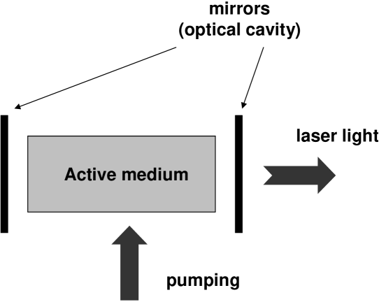
Figure 1: Scheme of a typical laser in a Fabry–Perot cavity.

A typical laser consists of three basic elements: An optical cavity, an amplifying medium, and a pumping mechanism, see Fig. 1. The optical cavity (also named resonator or oscillator) consists of two or more mirrors that force light to propagate in a closed circuit, further imposing it a certain modal structure. There are two basic types of optical cavities, namely ring and linear, that differ in the boundary condition that the cavity mirrors impose to the intracavity field. In ring resonators the field inside the cavity can be described as a traveling wave . Contrarily, in linear (also named Fabry–Perot–type) resonators, the field is better described as a standing wave, which requires a more complicated mathematical description than the traveling wave case.

The amplifying medium can be solid, liquid, gas, or plasma. Nevertheless, most cases are well described by considering that the amplifying medium consists of a number of atoms, ions or molecules of which a number of states (energy levels), with suitable relaxation rates and dipolar momenta, are involved in the interaction with the electromagnetic field. It is customary to adopt the so–called two–level approximation, i.e., to assume that only two energy levels of the amplifying medium are relevant for the interaction. Actually a minimum of three or four levels are necessary in order to obtain population inversion, and we discuss below how the two–level theory applies to these more complicated level schemes.

Then there is the pumping mechanism. This is highly specific for each laser type but it has always the same purpose: Creating enough population inversion for laser action. When modeling radiation–matter interaction inside the laser cavity one can usually forget the specifics of the pumping mechanism (whether it is an electric current or a broadband optical discharge or whatever) and describe it through a suitable pumping parameter. In this point, the consideration of two–, three– or four–level atomic schemes turns out to be important, as it is here where the pumping mechanism affects the mathematical description as we show below.

Laser physics studies all of these aspects of lasers but here we shall not deal but with the mathematical description of the interaction between light and matter inside the laser cavity. In this article we shall provide a systematic derivation of the semiclassical laser equations for an important and simple case: The homogeneously broadened ring laser, which plays the role of a paradigm in laser physics. We shall not consider the important issues of inhomogeneous broadening or linear optical resonators, because we want to maintain the derivation as simple as possible (but not more!).

As stated, we shall use semiclassical theory, i.e., we shall consider a classical electromagnetic field in interaction with a quantized medium. The quantization of the medium is necessary in order to correctly describe absorption and amplification as the classical theory (that models matter as a collection of forced and damped harmonic oscillators) cannot be used for that. With respect to the quantization of the field, it is not necessary if one (i) is not interested in the field fluctuations, and (ii) accepts a heuristic description of relaxation phenomena (in particular of spontaneous emission). In any case, the quantum theory of the laser requires the use of complicated mathematical techniques and falls outside the scope of our interests here.

After this introduction the rest of the article is organized as follows: In Section II we derive the field equation; in Section III we derive the matter equations for two–, three–, and four–level atoms or molecules; and in Section IV we connect these with the field equation and write down the Maxwell–Bloch equations. Then Sections V and VI are devoted to the analysis of amplification and lasing, respectively. In Section VII we present a clear derivation of the uniform field equations, and in Section VIII we present the ”Lorenz” from of the laser equations. Finally, in Section IX we present our conclusions.

II The Field Equation

Maxwell’s equations for a nonmagnetic material without free charges yield the wave equation

$$\boldsymbol{\nabla}^{2}\mathbf{E}-c^{-2}\partial_{t}^{2}\mathbf{E}+\boldsymbol{\nabla}\left(\boldsymbol{\nabla}\cdot\mathbf{E}\right)=\mu_{0}\partial_{t}^{2}\mathbf{P}.$$ (1)

Along this article we shall assume that the electric field $\mathbf{E}$ is a plane wave propagating along the $z$ axis, and write it in the form

$$\mathbf{E}\left(\mathbf{r},t\right)=\tfrac{1}{2}\mathbf{e}\mathcal{E}\left(z,t\right)e^{i\left(kz-\omega t\right)}+c.c.,$$ (2)

where $\mathbf{e}$ is the unit polarization vector (fixed polarization is assumed), and

$$k=\omega/c.$$ (3)

We note that $\omega$ is an arbitrary reference (carrier) frequency. For instance, if light is perfectly monochromatic of frequency $\omega_{0}$ we can still choose $\omega\neq\omega_{0}$ as we allow the complex amplitude $\mathcal{E}\left(z,t\right)$ to be time and space dependent. The situation is even clearer when dealing with light whose spectrum has some finite width: In this case even the concept of ”light frequency” is ill-defined, and clearly $\omega$ can be chosen arbitrarily.

Given the form (2) for the electric field, by consistency with the wave equation, the polarization $\mathbf{P}$ must read

$$\mathbf{P}\left(\mathbf{r},t\right)=\tfrac{1}{2}\mathbf{e}\mathcal{P}\left(z,t\right)e^{i\left(kz-\omega t\right)}+c.c..$$ (4)

Now one must substitute these expressions into the wave equation and perform the Slowly Varying Envelope Approximation (SVEA) that consists in assuming that

$$\partial_{t}^{2}U \ll\omega\partial_{t}U\ll\omega^{2}U,$$ (5)

$$\partial_{z}^{2}U \ll k\partial_{z}U\ll k^{2}U,$$ (6)

for $U=\mathcal{E}$ or $\mathcal{P}$. The physical meaning of this important approximation is clear: One considers that temporal (spatial) variations of the amplitudes $U$ contain temporal (spatial) frequencies that are much smaller than the carrier frequency (wavenumber). In other words: The amplitudes $U$ are assumed to vary on time (space) scales much slower (longer) than the optical frequency (wavelength). Obviously this approximation excludes the (limit) case of ultrashort pulses containing only a few cycles of the field, but it is overall very accurate in general, even for short pulses as soon as a sufficient number of cycles enter within the pulse width.

After performing the SVEA and multiplying the resulting equation by $c^{2}/2i\omega$, one readily obtains

$$\left(\partial_{t}+c\partial_{z}\right)\mathcal{E}=i\frac{\omega}{2\varepsilon_{0}}\mathcal{P},$$ (7)

which is the field equation of interest. Let us remark that the SVEA is a fundamental approximation in laser theory as it allows to transform the original wave equation, which is a second-order partial differential equation (PDE), into a first-order PDE.

Now we need to calculate the source term $\mathcal{P}$ and we do this in the next section.

III The matter equations: optical Bloch equations

The wave equation (7) relates the slowly varying electric field amplitude $\mathcal{E}$ with its source, the slowly varying polarization amplitude $\mathcal{P}$. We discuss in this section how this last quantity is determined. First we introduce the two–level atom model and derive the evolution equation for its density matrix, the so-called optical Bloch equations. Next, the density matrix is shown to yield the information necessary for computing $\mathcal{P}$ what allows to write a closed set of equations describing the coupled evolution of field and matter, the Maxwell–Bloch equations. Then we consider the case of three– and four–level atoms, which is a more realistic approximation to actual lasers. After deriving their corresponding Bloch equations, we discuss the conditions under which the two–level model can be applied to three– and four–level atoms. In particular this is a necessary step for correctly understand the meaning of the pump parameter.

III.1 The two–level atom model

III.1.1 Hamiltonian

The Hamiltonian of the system consists of two pieces: One describing the atom or molecule in the absence of electromagnetic interaction, and the other describing the action of the electromagnetic field on this atom, i.e.

$$H\left(\mathbf{r},t\right)=H_{\mathrm{at}}+H_{\mathrm{int}}\left(\mathbf{r},t\right).$$ (8)

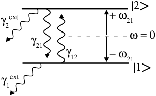
Figure 2: Schematic of the two–level atom energy levels including relaxation rates (see text)

The material medium is assumed to be a system of identical two–level atoms or molecules, i.e., it is assumed that the material medium is homogeneously broadened. We denote by $\left|1\right\rangle$ and $\left|2\right\rangle$ the lower and higher energy levels, respectively, and by $\omega_{21}$ the transition frequency of one of these atoms. This means that the atomic Hamiltonian $H_{\mathrm{at}}$ verifies

$$H_{\mathrm{at}}\left|2\right\rangle =+\tfrac{1}{2}\hbar\omega_{21}\left|2\right\rangle,$$ (9)

$$H_{\mathrm{at}}\left|1\right\rangle =-\tfrac{1}{2}\hbar\omega_{21}\left|1\right\rangle,$$ (10)

where we have chosen the arbitrary (and unimportant) energy origin in such a way that it lies halfway between both states energies (see, Fig. 2). The matrix representation for this Hamiltonian thus reads

$$H_{\mathrm{at}}=\begin{bmatrix}+\tfrac{1}{2}\hbar\omega_{21}&0\\ 0&-\tfrac{1}{2}\hbar\omega_{21}\end{bmatrix},$$ (11)

where the level ordering has been chosen to be $\left\{\left|2\right\rangle,\left|1\right\rangle\right\}$.

The interaction Hamiltonian $H_{\mathrm{int}}$ is taken in the electric dipole approximation. Roughly speaking, this approximation is valid when the light wavelength is much longer than the typical dimensions of the electronic cloud, which is on the order of $1$ $\operatorname{\text{\AA}}$. Thus the approximation is justified in the infrared and visible parts of the spectrum and even in the ultraviolet. This interaction hamiltonian reads

$$H_{\mathrm{int}}\left(\mathbf{r},t\right)=-\boldsymbol{\hat{\mu}}\cdot\mathbf{E}\left(\mathbf{r},t\right),$$ (12)

where $\mathbf{r}$ denotes the position of the atom (which is not quantized in the theory) and the operator $\boldsymbol{\hat{\mu}}=-e\mathbf{\hat{r}}_{\mathrm{at}}$, being $-e$ the electron charge and $\mathbf{\hat{r}}_{\mathrm{at}}$ the vector position operator of the electron relative to the point-like nucleus. $\boldsymbol{\hat{\mu}}$ acts on the atomic variables whereas in this semiclassical formalism the field $\mathbf{E}$ is a c-number. In the chosen basis ordering the matrix form for this hamiltonian reads

$$H_{\mathrm{int}}\left(\mathbf{r},t\right)=\begin{bmatrix}-\boldsymbol{\mu}_{22}\cdot\mathbf{E}\left(\mathbf{r},t\right)\ \ &-\boldsymbol{\mu}_{21}\cdot\mathbf{E}\left(\mathbf{r},t\right)\\ -\boldsymbol{\mu}_{12}\cdot\mathbf{E}\left(\mathbf{r},t\right)\ \ &-\boldsymbol{\mu}_{11}\cdot\mathbf{E}\left(\mathbf{r},t\right)\end{bmatrix},$$ (13)

where the matrix elements

$$\boldsymbol{\mu}_{mn}=\left\langle m\right|\boldsymbol{\hat{\mu}}\left|n\right\rangle\equiv-e\int d^{3}r_{\mathrm{at}}\ \psi_{m}^{\ast}\left(\mathbf{\hat{r}}_{\mathrm{at}}\right)\mathbf{\hat{r}}_{\mathrm{at}}\psi_{n}\left(\mathbf{\hat{r}}_{\mathrm{at}}\right),$$ (14)

and $\psi_{n}\left(\mathbf{\hat{r}}_{\mathrm{at}}\right)$ is the wavefunction (in position representation) of the atomic state $\left|n\right\rangle$. (Note that $\boldsymbol{\mu}_{mn}=\boldsymbol{\mu}_{nm}^{\ast}$.) We now recall the parity property of atomic eigenstates: All atomic eigenstates have well defined parity (even or odd) due to the central character of the atomic potential. This means that $\boldsymbol{\mu}_{11}=\boldsymbol{\mu}_{22}=0$ and then, in order to have interaction, we must consider states $\left|1\right\rangle$ and $\left|2\right\rangle$ with opposite parity (this is the basic selection rule of atomic transitions in the electric dipole approximation). Hence the interaction hamiltonian (13) becomes

$$H_{\mathrm{int}}\left(\mathbf{r},t\right)=\begin{bmatrix}0&V\left(\mathbf{r},t\right)\\ V^{\ast}\left(\mathbf{r},t\right)&0\end{bmatrix},$$ (15)

where we have introduced the notation

$$V\left(\mathbf{r},t\right)=-\boldsymbol{\mu}_{21}\cdot\mathbf{E}\left(\mathbf{r},t\right).$$ (16)

Taking into account the form of the electric field, Eq. (2), $V\left(\mathbf{r},t\right)$ becomes

$$V\left(\mathbf{r},t\right)=-\hbar\alpha\left(z,t\right)e^{i\left(kz-\omega t\right)}-\hbar\beta\left(z,t\right)e^{-i\left(kz-\omega t\right)},$$ (17)

where we have defined

$$\alpha\left(z,t\right)=\frac{\boldsymbol{\mu}_{21}\cdot\mathbf{e}}{2\hbar}\mathcal{E}\left(z,t\right),\qquad\beta\left(z,t\right)=\frac{\boldsymbol{\mu}_{21}\cdot\mathbf{e}^{\ast}}{2\hbar}\mathcal{E}^{\ast}\left(z,t\right).$$ (18)

We note that $2\alpha$ is usually referred to as the (complex) Rabi frequency of the light field.

Finally the total hamiltonian $H$, Eq. (8), for a two–level atom located at position $\mathbf{r}$ interacting with a light field reads

$$H\left(\mathbf{r},t\right)=\begin{bmatrix}+\tfrac{1}{2}\hbar\omega_{21}\ \ &V\left(\mathbf{r},t\right)\\ V^{\ast}\left(\mathbf{r},t\right)\ \ &-\tfrac{1}{2}\hbar\omega_{21}\end{bmatrix}.$$ (19)

III.1.2 The density matrix. Evolution

The hamiltonian $H$ can serve us to write down the Schrödinger equation for the atomic wavefunction. Instead, we use here the density matrix formalism as it is the most appropriate in order to incorporate damping and pumping terms into the equations of motion, something we shall do in the next subsection. In the chosen basis ordering, the density matrix $\rho$ representing a two–level atom located at $\mathbf{r}$ takes the form

$$\rho\left(\mathbf{r},t\right)=\begin{bmatrix}\rho_{22}\left(\mathbf{r},t\right)\ \ &\rho_{21}\left(\mathbf{r},t\right)\\ \rho_{12}\left(\mathbf{r},t\right)\ \ &\rho_{11}\left(\mathbf{r},t\right)\end{bmatrix}.$$ (20)

The meaning of the matrix elements is as follows: $\rho_{mm}$ denotes the probability ($0\leq\rho_{mm}\leq 1$) that the atom occupies state $\left|m\right\rangle$, and $\rho_{mn}\left(=\rho_{nm}^{\ast}\right)$ is the coherence between the two atomic states, which is related with the polarization induced in the the atom by the light field; see below. The evolution of $\rho$ is governed by the Schrödinger–von Neumann equation

$$i\hbar\partial_{t}\rho=\left[H,\rho\right].$$ (21)

Upon substituting Eqs. (20) and (19) into Eq. (21) one obtains a set of equations which is simplified by defining the new variables

$$\sigma_{12}=\sigma_{21}^{\ast}=\rho_{12}e^{i\left(kz-\omega t\right)}.$$ (22)

This is motivated by the functional dependence of the nondiagonal elements $\rho_{12}$ and $\rho_{21}$ on space and time under free evolution ($V=0$). (We note that the above transformation is equivalent to working in the so-called interaction picture of quantum mechanics.) The explicit space-time dependence added in Eq. (22) makes that the new quantities $\sigma_{ij}$ are slowly varying as will become evident later. In terms of these reduced density matrix elements, and making use of Eq. (17), the Schrödinger–von Neumann equation (21) becomes

$$\partial_{t}\rho_{22} =i\alpha\sigma_{12}+i\beta\sigma_{12}e^{-2i\left(kz-\omega t\right)}+c.c.,$$ (23)

$$\partial_{t}\rho_{11} =-i\alpha\sigma_{12}-i\beta\sigma_{12}e^{-2i\left(kz-\omega t\right)}+c.c.,$$ (24)

$$\partial_{t}\sigma_{12} =-i\delta\sigma_{12}+i\left(\rho_{22}-\rho_{11}\right)\left[\alpha^{\ast}+\beta^{\ast}e^{2i\left(kz-\omega t\right)}\right],$$ (25)

where we have introduced the mistuning, or detuning, parameter

$$\delta=\omega-\omega_{21}.$$ (26)

Note that $\partial_{t}\left(\rho_{22}+\rho_{11}\right)=0$, what implies probability conservation.

We now make a most important and widely used approximation in quantum optics, namely the Rotating Wave Approximation (RWA). An inspection of Eqs. (23)–(25) shows that, in the absence of interaction ($\mathcal{E}=0$, i.e. $\alpha=\beta=0$ in the new notation), $\rho_{22}$ and $\rho_{11}$ are constant and $\sigma_{12}=\sigma_{21}^{\ast}$ oscillate at the low (non optical) frequency $\delta$. This means that the time scales of the free system are large as compared with the optical periods. Now, if the interaction is turned on we see in Eqs. (23)–(25) that slowly varying terms (those proportional to $\alpha$ or $\alpha^{\ast}$) appear, as well as high frequency terms oscillating as $\exp\left[\pm 2i\left(kz-\omega t\right)\right]$ (the terms proportional to $\beta$ or $\beta^{\ast}$). Clearly the atom cannot respond to the latter and one can discard them. This is the RWA, which can be easily demonstrated by using perturbation theory.

After performing the RWA, Eqs. (23)–(25) become

$$\partial_{t}\rho_{22} =i\left(\alpha\sigma_{12}-\alpha^{\ast}\sigma_{21}\right),$$ (27)

$$\partial_{t}\rho_{11} =-i\left(\alpha\sigma_{12}-\alpha^{\ast}\sigma_{21}\right),$$ (28)

$$\partial_{t}\sigma_{12} =-i\delta\sigma_{12}+i\alpha^{\ast}\left(\rho_{22}-\rho_{11}\right),$$ (29)

which is the standard form of the optical Bloch equations for a single atom.

III.1.3 The population matrix

We are dealing with a situation in which there is not a single atom or molecule interacting with the light field but a very large number of them, and then some ensemble averaging must be performed. The ensemble averaged density matrix is called the population matrix Sargent , although the name density matrix is more frequently used obscuring the differences between the two operators. Here we are not going to introduce the population matrix rigorously and we refer the interested reader to Sargent or Meystre for further details.

The population matrix of an ensemble of molecules is defined as

$$\bar{\rho}\left(z,t\right)=\mathcal{N}^{-1}{\textstyle\sum_{a}}\rho_{a}\left(z,t\right).$$ (30)

Here $\bar{\rho}$ is the population matrix, $\rho_{a}$ is the density matrix for an atom labeled by $a$, and $a$ runs along all molecules that, at time $t$, are within $z$ and $z+dz$ . $\mathcal{N}$ is the number of such molecules, which is assumed to be independent of $z$ and $t$. The equation of evolution of the population matrix has two contributions: One of them is formally like the Schrödinger–von Neumann equation governing the evolution of the density matrix of a single atom, and the other one describes incoherent processes (i.e. not due to the interaction with the electromagnetic field such as pumping and relaxation phenomena due to collisions between atoms or to spontaneous emission) Sargent

$$\partial_{t}\bar{\rho}_{ij}=\left(i\hbar\right)^{-1}\left[H,\bar{\rho}\right]_{ij}+\left(\hat{\Gamma}\bar{\rho}\right)_{ij},$$ (31)

$\left(i,j=1,2\right)$. In Eq. (31) the term $\hat{\Gamma}\bar{\rho}$ is the one describing incoherent processes and $\hat{\Gamma}$ is the Liouville (super)operator.

Consider the situation depicted in Fig. 2. It corresponds to the following matrix elements for the operator $\left(\hat{\Gamma}\bar{\rho}\right)$

$$\left(\hat{\Gamma}\bar{\rho}\right)_{22} =-\gamma_{2}\bar{\rho}_{22}+\gamma_{12}\bar{\rho}_{11}+\lambda_{2},$$

$$\left(\hat{\Gamma}\bar{\rho}\right)_{21} =\left(\hat{\Gamma}\bar{\rho}\right)_{12}^{\ast}=-\gamma_{\bot}\bar{\rho}_{21},$$ (32)

$$\left(\hat{\Gamma}\bar{\rho}\right)_{11} =-\gamma_{1}\bar{\rho}_{11}+\gamma_{21}\bar{\rho}_{22}+\lambda_{1},$$

where

$$\gamma_{2} =\gamma_{2}^{ext}+\gamma_{21},$$ (33)

$$\gamma_{1} =\gamma_{1}^{ext}+\gamma_{12}.$$ (34)

In the above expressions, $\gamma_{ij}$ describes the relaxation rate from level $\left|i\right\rangle$ to level $\left|j\right\rangle$ (that is, the pass of population from level $\left|i\right\rangle$ to level $\left|j\right\rangle$ due to collisions), and $\gamma_{i}^{ext}$ the relaxation rate from level $\left|i\right\rangle$ to some other external level (see Fig. 2). The term $\lambda_{i}$ is the pumping rate of level $\left|i\right\rangle$, i.e., it describes the increase of population of level $\left|i\right\rangle$ due to pumping processes. Notice that it is not specified from where this population is coming as only the dynamics of the two lasing level populations is being described. We shall come back to this important point in the following subsection.

The value of the different decay constants appearing in $\hat{\Gamma}\bar{\rho}$ depend strongly on the particular substance and operating conditions. In any case it is always verified that

$$\gamma_{\bot}\geq\frac{1}{2}\left(\gamma_{2}+\gamma_{1}\right),$$ (35)

what reflects the fact that the coherence $\rho_{ij}$ is affected not only by the relaxation mechanisms affecting the populations, but also by some specific collisions, known as dephasing collisions, which do not affect the populations.

With the above form for the Liouvillian, the population matrix equations of evolution read

$$\partial_{t}\rho_{22} =-\gamma_{2}\rho_{22}+\gamma_{12}\rho_{11}+\lambda_{2}+i\left(\alpha\sigma_{12}-\alpha^{\ast}\sigma_{21}\right),$$ (36)

$$\partial_{t}\rho_{11} =-\gamma_{1}\rho_{11}+\gamma_{21}\rho_{22}+\lambda_{1}-i\left(\alpha\sigma_{12}-\alpha^{\ast}\sigma_{21}\right),$$ (37)

$$\partial_{t}\sigma_{12} =-\left(\gamma_{\bot}+i\delta\right)\sigma_{12}+i\alpha^{\ast}\left(\rho_{22}-\rho_{11}\right),$$ (38)

where we have removed the overbar in order not to complicate unnecessarily the notation. Now $\rho_{ii}$ can be understood as the fraction of atoms occupying level $\left|i\right\rangle$, i.e., it is the population of this level. Notice that in Eqs. (36-38) $\partial_{t}\left(\rho_{22}+\rho_{11}\right)\neq 0$ in general, what reflects the fact that the system formed by the atomic levels $\left|2\right\rangle$ and $\left|1\right\rangle$ is an open system in which population is gained and lost through incoherent processes.

In the two–level laser model, internal relaxation processes (those governed by $\gamma_{21}$ and $\gamma_{12}$) are usually neglected, and it is further assumed that the two lasing levels relax to the external reservoir with the same rate $\gamma_{||}=\gamma_{2}^{ext}=\gamma_{1}^{ext}$. It is easy to see that in this simplified description of relaxation processes, the pumping rates

$$\lambda_{i}=\frac{\rho_{ii}^{0}}{\gamma_{||}},$$ (39)

with $\rho_{ii}^{0}$ the population of level $\left|i\right\rangle$ in absence of fields ($\alpha=0$). Moreover, in this particular case $\partial_{t}\left(\rho_{22}+\rho_{11}\right)=0$ and then a single equation is needed for the description of the populations evolution. The population difference is then defined

$$d=\rho_{22}-\rho_{11},$$ (40)

and Eqs. (36-38) simplify to

$$\partial_{t}d =\gamma_{||}\left(d_{0}-d\right)+2i\left(\alpha\sigma_{12}-\alpha^{\ast}\sigma_{21}\right),$$ (41)

$$\partial_{t}\sigma_{12} =-\left(\gamma_{\bot}+i\delta\right)\sigma_{12}+i\alpha^{\ast}d,$$ (42)

where

$$d_{0}=\rho_{22}^{0}-\rho_{11}^{0},$$ (43)

is the population difference in the absence of fields, that is, the pump parameter. This is the simplest way of modeling pumping. Clearly, $d_{0}>0$ implies an inverted medium (with a larger number of excited atoms than of atoms in the fundamental state). If pumping is absent $d_{0}=-1$. Notice that $d_{0}$ appears as a free parameter, that we can take positive or negative, although we have not discussed yet how could it be controlled.

III.1.4 Rate Equations

It is interesting to write down Eqs. (36-38) when $\gamma_{\bot}\gg\gamma_{||},\delta$ as in this case the adiabatic elimination of the atomic polarization is justified (see Appendix 1). This adiabatic elimination consists in making $\partial_{t}\sigma_{12}=0$, and then Eqs. (36-38) reduce to

$$\partial_{t}\rho_{22} =\lambda_{2}-\gamma_{2}\rho_{22}+\gamma_{12}\rho_{11}-R\left(\rho_{22}-\rho_{11}\right),$$ (44)

$$\partial_{t}\rho_{11} =\lambda_{1}-\gamma_{1}\rho_{11}+\gamma_{21}\rho_{22}+R\left(\rho_{22}-\rho_{11}\right),$$ (45)

with $R=2\left|\alpha\right|^{2}/\gamma_{\bot}.$

These equations are known as rate equations and are widely used in laser physics as in most laser systems the condition for adiabatic elimination is met. Let us remark that rate equations describe appropriately the interaction of a light field with a two–level system in two limiting cases: When the atomic polarization can be adiabatically eliminated, as we have discussed, and also when the field is broadband (i.e., incoherent) in which case the factor $R$ has a different expression to the one we have derived but again depends on the square of the field amplitude deValcarcel04 . We shall make use of these equations in the following subsection.

III.2 Three–level and four–level atom models

As we already commented in the introduction, actual lasers are based on a three–level or four–level scheme rather than a two–level one, the extra levels describing the reservoirs from which the pump extracts atoms and to which damping sends atoms. In fact this extra levels are necessary for obtaining population inversion ($d_{0}>0$) which is a necessary condition for amplification and lasing, as we show below. Although these extra levels do not participate directly in laser action, the description of its indirect participation is essential in order to correctly describe pumping and decaying processes. Here we shall derive the Bloch equations for three–level and four–level atoms interacting with a laser field and an incoherent pump, and connect these equations with the two–level laser equations derived in the previous section.

III.2.1 Bloch equations for three–level atoms

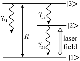
Figure 3: Schematic of a three–level atom. $R$ represents the incoherent pumping and the laser field interacts with the $\left|2\right\rangle\rightarrow\left|1\right\rangle$ transition. The arrows indicate decay processes.

Consider the three–level atom scheme depicted in Fig. 3, which can be regarded as an approximate description of, e.g., the relevant atomic levels of the Cr³⁺or the Er³⁺ ions that are the active ions in Ruby and Erbium lasers, respectively. On these ions population is excited from the lower state $\left|1\right\rangle$ to the upper state $\left|3\right\rangle$ by the pumping mechanism. Then population is transferred from level $\left|3\right\rangle$ to the upper lasing level $\left|2\right\rangle$ (which is long–lived) by relaxation processes, which are extremely fast in these ions.

We shall model the pumping transition $\left|1\right\rangle\longleftrightarrow\left|3\right\rangle$ via rate equations like Eqs. (44,45), and the interaction of the monochromatic field with transition $\left|1\right\rangle\longleftrightarrow\left|2\right\rangle$ with the already derived Bloch equations for a two–level atom. As for the relaxation processes, we describe them heuristically, see Fig. 3. Then we can model these processes with the following set of Bloch equations

$$\partial_{t}\rho_{33} =-\left(\gamma_{31}+\gamma_{32}\right)\rho_{33}+R\left(\rho_{11}-\rho_{33}\right),$$ (46)

$$\partial_{t}\rho_{22} =-\gamma_{21}\rho_{22}+\gamma_{32}\rho_{33}+i\left(\alpha\sigma_{12}-\alpha^{\ast}\sigma_{21}\right),$$ (47)

$$\partial_{t}\rho_{11} =\gamma_{21}\rho_{22}+\gamma_{31}\rho_{33}+R\left(\rho_{33}-\rho_{11}\right)$$ (48)

$$-i\left(\alpha\sigma_{12}-\alpha^{\ast}\sigma_{21}\right),$$

$$\partial_{t}\sigma_{12} =-\left(\gamma_{\bot}+i\delta\right)\sigma_{21}+i\alpha^{\ast}\left(\rho_{22}-\rho_{11}\right),$$ (49)

where $R$ is the rate at which ions are pumped by the incoherent pump field from level $\left|1\right\rangle$ to level $\left|3\right\rangle$. Let us remark that in writing Eqs. (46) and (48): (i), we have taken into account all possible transitions due to incoherent processes with suitable relaxation rates as indicated in Fig. 3; and (ii), the incoherent pumping of population from level $\left|1\right\rangle$ to level $\left|3\right\rangle$ is modelled by the term $R\left(\rho_{11}-\rho_{33}\right)$ appearing in Eqs. (46) and (48) with $R$ proportional to the pump intensity, i.e., we have described the interaction of the pump field with the pumped transition by means of rate equations similar to Eqs. (44) and (45) but taking $\lambda_{i}=0$ as all incoherent processes have been consistently taken into account.

Let us further assume that $\gamma_{32}\gg\gamma_{21},\gamma_{31},\gamma_{\bot},R$, as it occurs in usual three–level lasers. Then we adiabatically eliminate the population of level $\left|3\right\rangle$. By making $\partial_{t}\rho_{33}=0$ we get

$$\rho_{33}\approx\frac{R\rho_{11}}{\gamma_{32}}.$$ (50)

This equation shows that $\gamma_{32}\rho_{33}$ is a finite quantity; that is, $\rho_{33}$ is vanishingly small in the limit we are considering. Then we can neglect $\rho_{33}$ in Eq. (48) and put $\gamma_{32}\rho_{33}=R\rho_{11}$ in Eq. (47). By further noticing that after the approximation $\partial_{t}\left(\rho_{11}+\rho_{22}\right)=0$, we can write the simplified model

$$\partial d =R-\gamma_{21}-\left(R+\gamma_{21}\right)d+2i\left(\alpha\sigma_{12}-\alpha^{\ast}\sigma_{21}\right),$$ (51)

$$\partial_{t}\sigma_{12} =-\left(\gamma_{\bot}+i\delta\right)\sigma_{12}+i\alpha^{\ast}d,$$ (52)

where $d=\left(\rho_{22}-\rho_{11}\right)$. These are appropriate Bloch equations for most three–level systems.

Figure 4: Dependence of the effective pump parameter $d_{0}$ on the normalized actual pump strength $R/\gamma$ for three– (full line) and four–level (dashed line) lasers. $\gamma=\gamma_{21}$ for the three–level laser and $\gamma=\gamma_{20}+\gamma_{21}$ for the four–level laser.

We can now compare these equations that describe three–level atoms with Eqs. (41) and (42) that describe two–level atoms in a simple and usual limit. It is clear that they are isomorphic. Then we can conclude that incoherently pumped three–level atoms can be described with the standard two–level atom Bloch equations by making the following identifications

$$\gamma_{||} \rightarrow R+\gamma_{21},$$ (53)

$$d_{0} \rightarrow\frac{R-\gamma_{21}}{R+\gamma_{21}}.$$ (54)

Notice that (i) the decay rate $\gamma_{||}$ is pump dependent for three–level atoms, and (ii) that the pumping rate $d_{0}$ depends in a nonlinear way with the actual pump parameter $R$. In Fig. 4 we represent $d_{0}$ as a function of the actual pumping parameter $R$; notice that increasing $R$ in a factor ten, say, does not mean to do so in $d_{0}$. Apart from this, we have shown that an incoherently pumped three–level medium can be described as a two–level one when the adiabatic eliminations we have assumed are justified, which is the usual situation.

III.2.2 Bloch equations for four–level atoms

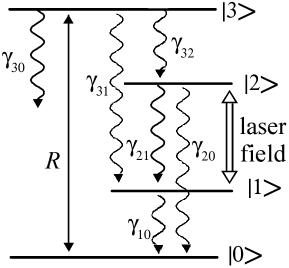
Figure 5: Schematic of a four–level atom. $R$ represents the incoherent pumping and the laser field interacts with the $\left|2\right\rangle\rightarrow\left|1\right\rangle$ transition. The arrows indicate decay processes.

Consider now the four–level atom scheme shown in Fig. 5. It can be regarded as an approximate description of, e.g., the relevant atomic levels of the $\mathrm{Nd}^{3+}$ ion that is the active ion Nd–YAG or Nd–glass lasers. Assuming, as for three–level atoms, that the pumping field acting on the transition $\left|0\right\rangle-\left|3\right\rangle$ can be described by rate equations, we are left with the following optical Bloch equations

$$\partial_{t}\rho_{33} =-\left(\gamma_{30}+\gamma_{31}+\gamma_{32}\right)\rho_{33}+R\left(\rho_{00}-\rho_{33}\right),$$ (55)

$$\partial_{t}\rho_{22} =-\left(\gamma_{20}+\gamma_{21}\right)\rho_{22}+\gamma_{32}\rho_{33}$$ (56)

$$+i\left(\alpha\sigma_{12}-\alpha^{\ast}\sigma_{21}\right),$$

$$\partial_{t}\rho_{11} =-\gamma_{10}\rho_{11}+\gamma_{21}\rho_{22}+\gamma_{31}\rho_{33}$$ (57)

$$+i\left(\alpha\sigma_{12}-\alpha^{\ast}\sigma_{21}\right),$$

$$\partial_{t}\rho_{00} =\gamma_{10}\rho_{11}+\gamma_{20}\rho_{22}+\gamma_{30}\rho_{33}-R\left(\rho_{00}-\rho_{33}\right)$$ (58)

$$\partial_{t}\sigma_{12} =-\left(\gamma_{\bot}+i\delta\right)\sigma_{21}+i\alpha^{\ast}\left(\rho_{22}-\rho_{11}\right).$$ (59)

We can now proceed in a similar way as we did with three–level atoms: Let us assume that $\gamma_{32}\$is much larger than any other decay rate and adiabatically eliminate $\rho_{33}$. Now we get

$$\rho_{33}\approx\frac{R\rho_{00}}{\gamma_{32}},$$ (60)

and neglecting the terms $\gamma_{31}\rho_{33},\gamma_{30}\rho_{33}$ and $R\rho_{33}$ we are left with

$$\partial_{t}\rho_{22} =-\left(\gamma_{20}+\gamma_{21}\right)\rho_{22}+R\rho_{00}$$ (61)

$$+i\left(\alpha\sigma_{12}-\alpha^{\ast}\sigma_{21}\right),$$

$$\partial_{t}\rho_{11} =-\gamma_{10}\rho_{11}+\gamma_{21}\rho_{22}+i\left(\alpha\sigma_{12}-\alpha^{\ast}\sigma_{21}\right),$$ (62)

$$\partial_{t}\rho_{00} =\gamma_{10}\rho_{11}+\gamma_{20}\rho_{22}-R\rho_{00}$$ (63)

$$\partial_{t}\sigma_{12} =-\left(\gamma_{\bot}+i\delta\right)\sigma_{21}+i\alpha^{\ast}\left(\rho_{22}-\rho_{11}\right).$$ (64)

Now we must take into account that the lower lasing level $\left|1\right\rangle$ usually relaxes very fast towards level $\left|0\right\rangle$. This means that $\rho_{11}\approx 0$ and consequently that $d=\rho_{22}-\rho_{11}\approx\rho_{22}$. Taking this into account and also that $\rho_{00}+\rho_{22}\approx 1$ in this approximation, we are left with

$$\partial_{t}\rho_{22} =-\left(\gamma_{20}+\gamma_{21}+R\right)d+R$$ (65)

$$+i\left(\alpha\sigma_{12}-\alpha^{\ast}\sigma_{21}\right),$$

$$\partial_{t}\sigma_{12} =-\left(\gamma_{\bot}+i\delta\right)\sigma_{21}+i\alpha^{\ast}d.$$ (66)

We see that, after the adiabatic elimination of $\rho_{33}$ and $\rho_{11}$, the four–level Bloch equations are isomorphic to Eqs. (41) and (42) that describe two–level atoms. Then we can apply the two–level description to a four–level atom by making the following identifications

$$\gamma_{||} \rightarrow\gamma_{20}+\gamma_{21}+R,$$ (67)

$$d_{0} \rightarrow\frac{R}{\gamma_{20}+\gamma_{21}+R}.$$ (68)

Again, as it was the case for three–level lasers, the population decay rate $\gamma_{||}$ and the pumping rate $d_{0}$ of the two–level theory must be reinterpreted when applied to four–level lasers.

Once we have shown that the two–level theory of Eqs. (41) and (42) can be applied to three– and four–level lasers by suitably interpreting the parameters $\gamma_{||}$ and $d_{0}$, in the following we shall always refer to the two–level model but the reader must keep in mind that the transformations we have derived must be taken into account when applying this theory to three– and four–level lasers.

IV The Maxwell–Bloch Equations

Once the field equation (7) and the optical Bloch equations for matter dynamics Eqs. (41) and (42) have been derived, we only need to connect them in order to obtain a closed set of equations for the analysis of amplification and laser dynamics.

Under the action of the light field each atom develops an electric dipole. As the number of atoms contained in a small volume (small as compared with the light wavelength) is always large, one can assume that at each spatial position $\mathbf{r}$ there exists a polarization given by the quantum-mechanical expectation value of the electric dipole moment operator $\boldsymbol{\hat{\mu}}$. When using the density (population) matrix formalism, this expectation value is computed as the trace

$$\mathbf{P}\left(\mathbf{r},t\right)=\mathcal{N}\mathrm{Tr}\left(\rho\left(\mathbf{r},t\right)\boldsymbol{\hat{\mu}}\right),$$ (69)

where $\mathcal{N}$ denotes the number of atoms per unit volume. Making use of Eq. (20) and of the matrix form for the dipole moment operator

$$\boldsymbol{\hat{\mu}}=\begin{bmatrix}0&\boldsymbol{\mu}_{21}\\ \boldsymbol{\mu}_{12}&0\end{bmatrix},$$

one has

$$\mathbf{P}\left(\mathbf{r},t\right)=\mathcal{N}\left[\boldsymbol{\mu}_{12}\rho_{21}\left(\mathbf{r},t\right)+c.c.\right],$$ (70)

which, making use of definitions (22), reads

$$\mathbf{P}\left(\mathbf{r},t\right)=\mathcal{N}\left[\boldsymbol{\mu}_{12}\sigma_{21}\left(\mathbf{r},t\right)e^{i\left(kz-\omega t\right)}+c.c.\right],$$ (71)

which, compared with Eq. (4) yields

$$\mathcal{P}\left(z,t\right)=2\mathcal{N}\left(\boldsymbol{\mu}_{12}\cdot\mathbf{e}^{\ast}\right)\sigma_{21}\left(\mathbf{r},t\right).$$ (72)

We finally come back to the wave equation (7), multiply it by $\left(\boldsymbol{\mu}_{21}\cdot\mathbf{e}\right)/2\hbar$, and make use of Eqs. (18) and (72) for obtaining the final field equation, which we write together with the Bloch equations (41)–(42) for the sake of convenience

$$\frac{\partial\alpha}{\partial t}+c\frac{\partial\alpha}{\partial z}=ig\sigma_{21},$$ (73)

$$\partial_{t}\sigma_{12}=-\left(\gamma_{\bot}+i\delta\right)\sigma_{12}+i\alpha^{\ast}d,$$ (74)

$$\partial_{t}d=\gamma_{||}\left(d_{0}-d\right)+2i\left(\alpha\sigma_{12}-\alpha^{\ast}\sigma_{21}\right),$$ (75)

where we have introduced the radiation–matter coupling constant

$$g=\frac{\mathcal{N}\omega\left|\boldsymbol{\mu}_{21}\cdot\mathbf{e}\right|^{2}}{2\varepsilon_{0}\hbar}\text{.}$$ (76)

Note that Eqs. (73–75), form a closed set of equations that completely determines, self-consistently, the interaction between a light field (of amplitude proportional to $\alpha$, see Eq. (18)) and a collection of two–level atoms. This set of equations is known as the Maxwell–Bloch equations for a two–level system, which can be applied to three– and four–level systems by introducing the parameter changes (53,54) and (67,68), respectively.

V Amplification

The simplest issue that can be studied within the developed formalism is the amplification of a monochromatic light beam after traveling some distance along a medium. If we identify $\omega$ with the actual light frequency, then $\mathcal{E}\left(z,t\right)=\mathcal{E}\left(z\right)$, see Eq. (2), which implies that $\alpha\left(z,t\right)=\alpha\left(z\right)$. On the other hand, after a short transient (of the order of the inverse of the decay constants), the atomic system will have reached a steady configuration, which is ensured by the presence of damping. Thus, after that transient one can ignore the time derivatives in the Maxwell–Bloch equations. Solving for the material variables (41)–(42) in steady state, one has

$$d_{\mathrm{s}} =d_{0}\frac{\gamma_{\bot}^{2}+\delta^{2}}{\delta^{2}+\gamma_{\bot}^{2}+4\gamma_{\bot}\left|\alpha\right|^{2}/\gamma_{||}},$$ (77)

$$\sigma_{21,\mathrm{s}} =d_{0}\alpha\frac{\delta-i\gamma_{\bot}}{\delta^{2}+\gamma_{\bot}^{2}+4\gamma_{\bot}\left|\alpha\right|^{2}/\gamma_{||}},$$ (78)

where the subscript ”$\mathrm{s}$” refers to the steady state. Substituting the result into the field equation (73) one has

$$\frac{d\alpha}{dz}=\frac{d_{0}g}{c}\frac{\gamma_{\bot}+i\delta}{\delta^{2}+\gamma_{\bot}^{2}+4\gamma_{\bot}\left|\alpha\right|^{2}/\gamma_{||}}\alpha.$$ (79)

This equation governs the spatial variation of the field amplitude $\alpha$ along the atomic medium.

V.1 Weak field limit

Before considering the general solution let us concentrate first on the weak field limit, defined as $\left|\alpha\right|^{2}\ll\gamma_{\bot}\gamma_{||}/4$. In this case the last term of the denominator in Eq. (79) can be ignored and the solution reads

$$\alpha\left(z\right)=\alpha\left(0\right)\exp\left[\frac{a/2}{1+\left(\delta/\gamma_{\bot}\right)^{2}}\ \left(1+i\frac{\delta}{\gamma_{\bot}}\right)z\right],$$ (80)

where

$$a=\frac{2d_{0}g}{c\gamma_{\bot}},$$ (81)

and $g$ given by Eq. (76). Parameter $a$ is responsible for the attenuation (when $a<0$, i.e., when $d_{0}<0$) or amplification ($a>0$, i.e., $d_{0}>0$) of the light along its propagation through the material. In case of attenuation, the inverse $a^{-1}$ is known as penetration depth. In case of amplification $a$ receives the name of small-signal gain per unit length. (Note that for $\delta=0$, $\left|\alpha\left(z\right)\right|^{2}=\left|\alpha\left(0\right)\right|^{2}\exp\left(az\right)$.)

On the other hand the imaginary exponent corresponds to a correction to the light wavenumber. In fact, noticing that $\alpha$ is proportional to the field amplitude $\mathcal{E}$ and recalling Eq. (2) one has that the actual wavenumber is

$$k_{\mathrm{eff}}=k+\delta k,$$ (82)

and consequently the refractive index $n=ck_{\mathrm{eff}}/\omega$ reads

$$n =\frac{ck}{\omega}+\frac{d_{0}g}{\gamma_{\bot}\omega}\frac{\left(\delta/\gamma_{\bot}\right)}{1+\left(\delta/\gamma_{\bot}\right)^{2}}$$

$$=1+\frac{d_{0}\mathcal{N}\left|\boldsymbol{\mu}_{21}\cdot\mathbf{e}\right|^{2}}{2\varepsilon_{0}\hbar\gamma_{\bot}}\frac{\left(\delta/\gamma_{\bot}\right)}{1+\left(\delta/\gamma_{\bot}\right)^{2}},$$ (83)

which has the same qualitative behavior as the classical expression obtained from the (harmonic oscillator) Lorentz model MilonniEberly .

V.2 Strong field limit

In the opposite limit, namely $\left|\alpha\right|^{2}\gg\gamma_{\bot}\gamma_{||}/4,\delta^{2}$, Eq. (79) becomes

$$\frac{d\alpha}{dz}=\frac{\gamma_{||}d_{0}g}{4c}\left(1+i\frac{\delta}{\gamma_{\bot}}\right)\frac{\alpha}{\left|\alpha\right|^{2}}.$$ (84)

Multiplying this equation by $\alpha^{\ast}$ and taking the real part of the resulting equation one has

$$\frac{d\left|\alpha\right|^{2}}{dz}=\frac{\gamma_{||}d_{0}g}{2c}=\frac{\gamma_{||}\gamma_{\bot}a}{4},$$ (85)

whose solution reads

$$\left|\alpha\left(z\right)\right|^{2}=\left|\alpha\left(0\right)\right|^{2}+\frac{\gamma_{||}\gamma_{\bot}a}{4}z.$$ (86)

Again, amplification requires $a>0$, i.e., $d_{0}>0$. This result means that, for strong fields, there exists saturation: the amplification (whenever $d_{0}>0$) persists but it is linear in the propagation distance, differently from the weak field limit, in which amplification occurs exponentially, see Eq. (80).

V.3 General solution

In order to consider the general case it is convenient to use a polar decomposition for $\alpha$ as

$$\alpha\left(z\right)=\left|\alpha\left(z\right)\right|e^{i\phi\left(z\right)}.$$ (87)

Substituting this expression into Eq. (79) and separating it into its real and imaginary parts one obtains

$$\frac{d\left|\alpha\right|}{dz} =\frac{\gamma_{\bot}d_{0}g}{c}\frac{\left|\alpha\right|}{\delta^{2}+\gamma_{\bot}^{2}+4\gamma_{\bot}^{2}\left|\alpha\right|^{2}/\gamma_{||}},$$ (88)

$$\frac{d\phi}{dz} =\frac{\delta d_{0}g}{c}\frac{1}{\delta^{2}+\gamma_{\bot}^{2}+4\gamma_{\bot}^{2}\left|\alpha\right|^{2}/\gamma_{||}}.$$ (89)

Figure 6: Field intensity during amplification as a function of the normalized distance $z/z_{pd}$, with $z_{pd}=a^{-1}$ the penetration depth. The dashed lines correspond to the weak and strong field approximations, Eqs. (80) and (86), respectively.

Eq. (88) can be integrated to yield

$$\left(\gamma_{\bot}^{2}+\delta^{2}\right)\ln\frac{\left|\alpha\left(z\right)\right|}{\left|\alpha\left(0\right)\right|}+2\frac{\gamma_{\bot}}{\gamma_{||}}\left[\left|\alpha\left(z\right)\right|^{2}-\left|\alpha\left(0\right)\right|^{2}\right]=\frac{\gamma_{\bot}d_{0}g}{c}z,$$ (90)

which does not allow an explicit expression for $\left|\alpha\left(z\right)\right|$. In any case, Eq. (88) shows that $\left|\alpha\left(z\right)\right|^{-1}d\left|\alpha\left(z\right)\right|/dz$ has the same sign as $d_{0}$, so that $d_{0}>0$ implies amplification. In Fig. 6 the solution of Eq. (90) is represented as a function of $z$ together with the weak and strong field approximations derived above.

As for Eq. (89), the phase can be determined by noticing that

$$\frac{d\phi}{d\left|\alpha\right|}=\frac{d\phi/dz}{d\left|\alpha\right|/dz}=\frac{\delta}{\gamma_{\bot}}\frac{1}{\left|\alpha\right|},$$ (91)

from which

$$\phi=\phi_{0}+\frac{\delta}{\gamma_{\bot}}\ln\frac{\left|\alpha\left(z\right)\right|}{\left|\alpha\left(0\right)\right|}.$$ (92)

Note that, on resonance ($\delta=\omega-\omega_{21}=0$) there is no phase variation along the propagation direction (apart from the original phase $kz$).

VI Lasing

Differently from the previous analysis, in which we assumed that a given field (whose frequency and initial amplitude are known data) is injected into the entrance face of a material, the light field in a laser is not fixed externally but is self-consistently generated by the medium, through amplification, and must verify the boundary conditions imposed by the cavity. As the model we have developed considers a traveling wave (moving in one direction) the following analysis only applies to ring lasers in which unidirectional operation can take place (in linear, i.e. Fabry–Perot, resonators there are two counterpropagating waves that form a standing wave, a more complicated case that we shall not treat here).

VI.1 Boundary condition

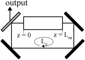
Figure 7: Scheme of the ring cavity. The active medium is placed in the region $0<z<L_{\mathrm{m}}$. The black cavity mirrors are perfectly reflecting whilst the grey mirror has a finite reflectivity $\mathcal{R}$. The arrows indicate the propagation of the intracavity and output fields.

We assume that the medium is of length $L_{\mathrm{m}}$ and that the cavity has a length $L_{\mathrm{c}}$, see Fig. 7. We take $z=0$ as the entrance face of the amplifying medium. The boundary condition imposed by the resonator reads

$$\mathbf{E}\left(0,t\right)=\mathcal{R}\mathbf{E}\left(L_{\mathrm{m}},t-\Delta t\right),$$ (93)

where $\mathcal{R}$ represents the (amplitude) reflectivity of the mirrors ($0\leq\mathcal{R}^{2}\leq 1$ gives the fraction of light power that survives after a complete cavity round trip) and

$$\Delta t=\frac{L_{\mathrm{c}}-L_{\mathrm{m}}}{c}$$ (94)

is the time delay taken by the light to travel from the exit face of the medium back to its entrance face after being reflected by the cavity mirrors.

Making use of Eq. (2), and after little algebra, the boundary condition (93) reads

$$\mathcal{E}\left(0,t\right)=\mathcal{R}\exp\left[i\left(kL_{\mathrm{m}}+\omega\Delta t\right)\right]\mathcal{E}\left(L_{\mathrm{m}},t-\Delta t\right),$$ (95)

which, upon using Eq. (94) and recalling that $k=\omega/c$ (this was our choice in writing Eq. (2)), reads

$$\mathcal{E}\left(0,t\right)=\mathcal{R}e^{ikL_{\mathrm{c}}}\mathcal{E}\left(L_{\mathrm{m}},t-\Delta t\right).$$ (96)

Finally, multiplying this equation by $\left(\boldsymbol{\mu}_{21}\cdot\mathbf{e}\right)/2\hbar$ and recalling Eq. (18), one has

$$\alpha\left(0,t\right)=\mathcal{R}e^{ikL_{\mathrm{c}}}\alpha\left(L_{\mathrm{m}},t-\Delta t\right).$$ (97)

We analyze next the monochromatic lasing solution.

VI.2 Monochromatic (singlemode) emission

We note that the frequency $\omega$ appearing in the field expression (2) is by now unknown. Under monochromatic operation the laser light has, by definition, a single frequency. If we take $\omega$ to be the actual lasing mode frequency, the field amplitude must be then a constant in time i.e., $\alpha\left(z,t\right)=\alpha\left(z\right)$, as in the previous analysis. Thus Eq. (97) becomes

$$\alpha\left(0\right)=\mathcal{R}e^{ikL_{\mathrm{c}}}\alpha\left(L_{\mathrm{m}}\right).$$ (98)

Using now the polar decomposition (87) one has

$$\left|\alpha\left(0\right)\right|^{2} =\mathcal{R}^{2}\left|\alpha\left(L_{\mathrm{m}}\right)\right|^{2},$$ (99)

$$\phi\left(0\right) =\phi\left(L_{\mathrm{m}}\right)+kL_{\mathrm{c}}+2m\pi,$$ (100)

being $m$ an integer.

VI.2.1 Determination of the laser intensity

Let us first analyze the laser intensity $\left|\alpha\right|^{2}$. (In fact the laser intensity is proportional to $\left|\mathcal{E}\right|^{2}$ but remind that $\mathcal{E}\propto\alpha$, and then $\left|\mathcal{E}\right|^{2}\propto\left|\alpha\right|^{2}$.) We note that, as we are dealing with a field whose amplitude is time independent, the analysis of amplification performed in the previous section is directly applicable. Making use of Eq. (99), Eq. (90) becomes, for $z=L_{\mathrm{m}}$,

$$\frac{\gamma_{\bot}d_{0}g}{c}L_{\mathrm{m}} =\frac{1}{2}\left(\gamma_{\bot}^{2}+\delta^{2}\right)\ln\mathcal{R}^{-2}$$

$$+2\frac{\gamma_{\bot}}{\gamma_{||}}\left(1-\mathcal{R}^{2}\right)\left|\alpha\left(L_{\mathrm{m}}\right)\right|^{2},$$ (101)

which, after trivial manipulation yields

$$\left|\alpha\left(L_{\mathrm{m}}\right)\right|^{2}=\frac{\gamma_{||}\gamma_{\bot}}{4}\frac{\left|\ln\mathcal{R}^{2}\right|}{1-\mathcal{R}^{2}}\left(r-1-\Delta^{2}\right),$$ (102)

where we made $\ln\mathcal{R}^{-2}=\left|\ln\mathcal{R}^{2}\right|$ (remind that $\mathcal{R}^{2}\leq 1$) and we have defined two important parameters, the adimensional pump $r$ and the normalized detuning $\Delta$ through

$$r =\frac{2d_{0}gL_{\mathrm{m}}}{\gamma_{\bot}c\left|\ln\mathcal{R}^{2}\right|}=\frac{aL_{\mathrm{m}}}{\left|\ln\mathcal{R}^{2}\right|},$$ (103)

$$\Delta =\frac{\delta}{\gamma_{\bot}}=\frac{\omega-\omega_{21}}{\gamma_{\bot}}.$$ (104)

We note that the adimensional parameter $r$ is proportional to the gain properties of the medium and inversely proportional to the damping properties of the system. In fact, $aL_{\mathrm{m}}$ gives the small-signal single-pass gain along the amplifying medium (remind that $a$, Eq. (81), is the small-signal gain per unit length). Thus $r$ acts as an effective pumping parameter, as will become clear next. Equation (102) determines the value of the field intensity at the exit face of the amplifying medium. Clearly, in order to be meaningful, $\left|\alpha\left(L_{\mathrm{m}}\right)\right|^{2}\geq 0$, what implies

$$r\geq r_{on}\equiv 1+\Delta^{2}.$$ (105)

Thus parameter $r$ must exceed a given threshold (the lasing threshold $r_{0}$) in order that the laser emits light. This is why $r$ is called the pump parameter (there is a minimum pump required for the system starts lasing).

Figure 8: Intracavity field intensity as a function of distance for $\gamma_{||}=\gamma_{\bot},\Delta=0,r=1.5$ and the values of $\mathcal{R}$ marked in the figure.

What we have obtained is the field intensity at the faces of the active medium, Eqs. (99) and (102). But it is also interesting to analyze how this intensity varies along the active medium. Thus, after using Eqs. (99), (103) and (104), we write down Eq. (90) in the form

$$r\left|\ln\mathcal{R}^{2}\right|\frac{z}{L_{\mathrm{m}}}=\left(1+\Delta^{2}\right)\ln\frac{\left|\alpha\left(z\right)\right|^{2}}{\mathcal{R}^{2}\left|\alpha\left(L_{\mathrm{m}}\right)\right|^{2}}$$

$$+\frac{4}{\gamma_{||}\gamma_{\bot}}\left[\left|\alpha\left(z\right)\right|^{2}-\mathcal{R}^{2}\left|\alpha\left(L_{\mathrm{m}}\right)\right|^{2}\right],$$ (106)

with $\left|\alpha\left(L_{\mathrm{m}}\right)\right|^{2}$ given by Eq. (102). This equation can be solved numerically and in Fig. 8 we represent its solutions for fixed parameters and several values of the reflectivity $\mathcal{R}^{2}$, showing that as $\mathcal{R}^{2}$ approaches unity the solution becomes progressively uniform. This fact suggests that for $\mathcal{R}^{2}\rightarrow 1$, it must be possible to rewrite the laser equations in a simpler way as in this limit the steady state is independent of $z$. We shall come back to this point in the next section. But first we shall continue analyzing the laser steady state.

VI.2.2 Determination of the laser frequency

Even if it can seem that we know the lasing intensity value, the fact is that we still ignore the value of the lasing frequency $\omega$ and thus the value of $\Delta$. This problem is solved by considering the phase boundary condition (100). First we recall Eq. (92), which we write in the form

$$\phi\left(L_{\mathrm{m}}\right)-\phi\left(0\right)=\tfrac{1}{2}\Delta\ln\frac{\left|\alpha\left(L_{\mathrm{m}}\right)\right|^{2}}{\left|\alpha\left(0\right)\right|^{2}}=-\tfrac{1}{2}\Delta\left|\ln\mathcal{R}^{2}\right|,$$ (107)

where Eq. (99) has been used in the last equality. Comparison between Eqs. (100) and (107) yields

$$\tfrac{1}{2}\Delta\left|\ln\mathcal{R}^{2}\right|=2\pi m-kL_{\mathrm{c}}.$$ (108)

We now introduce the wavenumber $k_{\mathrm{c}}$ and frequency $\omega_{\mathrm{c}}$ of the cavity longitudinal mode closest to the atomic resonance. As we are dealing with a cavity longitudinal mode, it must be verified, by definition, that

$$k_{\mathrm{c}}=2\pi m_{\mathrm{c}}/L_{\mathrm{c}},\qquad\omega_{\mathrm{c}}=ck_{\mathrm{c}},$$ (109)

being $m_{\mathrm{c}}$ an integer. Substituting these quantities into Eq. (108) one gets

$$\tfrac{1}{2}\Delta\left|\ln\mathcal{R}^{2}\right|=\left(\omega_{\mathrm{c}}-\omega\right)\frac{L_{\mathrm{c}}}{c}+2\pi n,$$ (110)

where $n=m-m_{\mathrm{c}}$ is a new integer. We finally recall Eq. (104) so that Eq. (110) yields the following value for the laser frequency

$$\omega_{n}=\frac{\kappa\omega_{21}+\gamma_{\bot}\omega_{\mathrm{c}}}{\kappa+\gamma_{\bot}}+n\frac{\gamma_{\bot}}{\kappa+\gamma_{\bot}}\frac{2\pi c}{L_{\mathrm{c}}}$$ (111)

where we have defined

$$\kappa=\frac{c\left|\ln\mathcal{R}^{2}\right|}{2L_{\mathrm{c}}},$$ (112)

which is known as the cavity damping rate for reasons that will be analyzed in the next section. We note that Eq. (111) indicates that there exists a family of solutions (labeled by the integer $n$). As we show next all these solutions have, in general, different lasing thresholds. From Eq. (111) the lasing threshold (105) can be finally determined as

$$r_{on}=1+\left(\frac{\omega_{\mathrm{c}}-\omega_{21}+n\frac{2\pi c}{L_{\mathrm{c}}}}{\kappa+\gamma_{\bot}}\right)^{2}.$$ (113)

Now, the difference between the cavity and atomic transition frequencies is obviously smaller than the free spectral range, i.e., $\left|\omega_{\mathrm{c}}-\omega_{21}\right|<2\pi c/L_{\mathrm{c}}$. This makes that $r_{on}$ is minimum for $n=0$ and, also, that the frequency of the amplified mode, $\omega_{0}$, be given by

$$\omega_{0}=\frac{\kappa\omega_{21}+\gamma_{\bot}\omega_{\mathrm{c}}}{\kappa+\gamma_{\bot}},$$ (114)

which is the pulling formula. The result is that the laser frequency is a compromise between the cavity and atomic transition frequency. Notice that for a ”good cavity”, $\kappa\ll\gamma_{\bot}$, the laser frequency approaches the cavity frequency, whilst for a ”bad cavity”, $\gamma_{\bot}\ll\kappa$, the laser frequency approaches that of the atomic transition. This is a quite intuitive result indeed.

VI.2.3 The resonant case

Let us analyze the relevant case $\omega_{\mathrm{c}}=\omega_{21}$, corresponding to a cavity exactly tuned to the atomic resonance. In this case the pump must verify

$$r\geq r_{on}=1+\left[\frac{2\pi c}{\left(\kappa+\gamma_{\bot}\right)L_{\mathrm{c}}}\right]^{2}n^{2},$$ (115)

and the lasing mode with lowest threshold is that with $n=0$, as discussed above. Hence, at resonance, the basic lasing solution has a threshold given by $r_{on}=1$, and its frequency is $\omega=\omega_{\mathrm{c}}=\omega_{21}$, see Eq. (111) for $n=0$.

The amplitude of this lasing solution verifies Eq. (79) with $\delta=\omega-\omega_{21}=0$:

$$\frac{d\alpha_{\mathrm{s}}}{dz}=\frac{d_{0}g}{\gamma_{\bot}c}\frac{1}{1+\frac{4}{\gamma_{\bot}\gamma_{||}}\left|\alpha_{\mathrm{s}}\right|^{2}}\alpha_{\mathrm{s}}.$$ (116)

We note that we have introduced the subscript ”$\mathrm{s}$” to emphasize that this amplitude $\alpha$ corresponds to the steady lasing solution.

Finally, the ”intensity” of the laser light at the exit of the active medium is given by Eq. (102) with $\Delta=\delta/\gamma_{\bot}=0$:

$$\left|\alpha_{\mathrm{s}}\left(L_{\mathrm{m}}\right)\right|^{2}=\frac{\gamma_{||}\gamma_{\bot}}{4}\frac{\left|\ln\mathcal{R}^{2}\right|}{1-\mathcal{R}^{2}}\left(r-1\right).$$ (117)

We note that there exists no phase variation of the laser complex amplitude $\alpha_{\mathrm{s}}$ along the medium, see Eq. (89) with $\delta=0$. We shall make use of these expressions in the following section.

VII The laser equations in the uniform field limit

In this section we want to find a simpler model that allows us to study laser dynamics and instabilities in an easy way. The sought model is known as the Lorenz–Haken model and can be rigorously derived from the Maxwell–Bloch equations (41)–(42) and (73) in the so-called uniform field limit, which we consider now. This limit assumes that the cavity reflectivity is closest to unity ($\mathcal{R}^{2}\rightarrow 1$ in all previous expressions). For the sake of simplicity nonresonant the derivation will be done in the resonant case, where the cavity is tuned in such a way that one of its longitudinal modes has a frequency $\omega_{\mathrm{c}}$ that matches exactly the atomic resonance frequency $\omega_{21}$. In this case the analysis done in Sec. (VI.2.3) suggests to choose the value of the arbitrary frequency $\omega$ as $\omega=\omega_{\mathrm{c}}=\omega_{21}$. (We remind that we can choose freely this value. If this election is ”wrong” the laser equations will yield an electric field amplitude $\alpha$ which contains a phase factor of the form $\exp\left(-i\Delta\omega t\right)$ that will define the actual laser frequency.)

First we recall the Maxwell–Bloch equations (73–75) for $\delta=0$:

$$\frac{\partial\alpha}{\partial t}+c\frac{\partial\alpha}{\partial z}=ig\sigma_{21},$$ (118)

$$\frac{\partial\sigma_{21}}{\partial t}=-\gamma_{\bot}\sigma_{21}-i\alpha d,$$ (119)

$$\frac{\partial d}{\partial t}=\gamma_{||}\left(d_{0}-d\right)+2i\left(\alpha\sigma_{12}-\alpha^{\ast}\sigma_{21}\right),$$ (120)

which are to be supplemented by the boundary condition (97) with $k=k_{\mathrm{c}}=\omega_{\mathrm{c}}/c$, see Eq. (3), so that $k=2\pi m_{\mathrm{c}}/L_{\mathrm{c}}$, see Eq. (109). With these assumptions the boundary condition (97) becomes

$$\alpha\left(0,t\right)=\mathcal{R}\alpha\left(L_{\mathrm{m}},t-\Delta t\right).$$ (121)

We note that this boundary condition is not isochronous (it relates values of the field amplitude at different times) and this makes difficult the analysis. We note for later use that this boundary condition applies, in particular, to the steady lasing solution (independent of time) so that

$$\alpha_{\mathrm{s}}\left(0\right)=\mathcal{R}\alpha_{\mathrm{s}}\left(L_{\mathrm{m}}\right).$$ (122)

These equations form the basis of our study.

VII.1 A first change of variables

In order to make the boundary condition isochronous, we introduce the following change of variables NarducciAbraham :

$$\alpha^{\prime}\left(z,t\right) =\alpha\left(z,t-\tau\right),\ \$$ (123)

$$\sigma_{21}^{\prime}\left(z,t\right) =\sigma_{21}\left(z,t-\tau\right),\ \$$ (124)

$$d^{\prime}\left(z,t\right) =d\left(z,t-\tau\right),$$ (125)

with $\tau=z\Delta t/L_{\mathrm{m}}$ and $\Delta t=\left(L_{\mathrm{c}}-L_{\mathrm{m}}\right)/c$, Eq. (94). The new variables verify

$$\frac{\partial\alpha}{\partial t} =\frac{\partial\alpha^{\prime}}{\partial t},$$ (126)

$$\frac{\partial\alpha}{\partial z} =\frac{\partial\alpha^{\prime}}{\partial z}+\frac{\Delta t}{L_{\mathrm{m}}}\frac{\partial\alpha^{\prime}}{\partial t},$$ (127)

and similar expressions for the material variables. Substitution of the previous relations into Eqs. (118)–(120) yields

$$\frac{L_{\mathrm{c}}}{L_{\mathrm{m}}}\frac{\partial\alpha^{\prime}}{\partial t}+c\frac{\partial\alpha^{\prime}}{\partial z}=ig\sigma_{21}^{\prime},$$ (128)

$$\frac{\partial\sigma_{21}^{\prime}}{\partial t}=-\gamma_{\bot}\sigma_{21}^{\prime}-i\alpha^{\prime}d^{\prime},$$ (129)

$$\frac{\partial d^{\prime}}{\partial t}=-\gamma_{||}\left(d^{\prime}-d_{0}\right)+2i\alpha^{\prime}\sigma_{12}^{\prime}+c.c.,$$ (130)

where we used Eq. (94). According to Eq. (121) the new variables verify the following boundary condition

$$\alpha^{\prime}\left(0,t\right)=\mathcal{R}\alpha^{\prime}\left(L_{\mathrm{m}},t\right),$$ (131)

which is now isochronous. We note that the definition of the new variables is mathematically equivalent to ”bend” the active medium on itself so that its entrance ($z=0$) and exit faces ($z=L_{\mathrm{m}}$) coincide.

VII.2 A second change of variables

Now we define another set of variables by referring the previous ones to their monochromatic lasing values analyzed in the previous sections. The steady values of the material variables have been calculated in Sec. (V), Eqs. (77) and (78), that, particularized to the case $\delta=0$ we are considering, read

$$d_{\mathrm{s}}\left(z\right) =d_{0}\frac{1}{1+\frac{4}{\gamma_{\bot}\gamma_{||}}\left|\alpha_{\mathrm{s}}\right|^{2}},$$ (132)

$$\sigma_{21,\mathrm{s}}\left(z\right) =\frac{-id_{0}\alpha_{\mathrm{s}}}{\gamma_{\bot}}\frac{1}{1+\frac{4}{\gamma_{\bot}\gamma_{||}}\left|\alpha_{\mathrm{s}}\right|^{2}}.$$ (133)

We note that these quantities are $z-$dependent as $\alpha_{\mathrm{s}}$ is, Eq. (116). In particular we define the new variables through

$$F\left(z,t\right) =\sqrt{r-1}\frac{\alpha^{\prime}\left(z,t\right)}{\alpha_{\mathrm{s}}\left(z\right)},\;$$ (134)

$$P\left(z,t\right) =\sqrt{r-1}\frac{\sigma_{21}^{\prime}\left(z,t\right)}{\sigma_{21,\mathrm{s}}\left(z\right)},$$ (135)

$$D\left(z,t\right) =\frac{d^{\prime}\left(z,t\right)}{d_{\mathrm{s}}\left(z\right)},$$ (136)

where $\alpha_{\mathrm{s}}$ verifies Eq. (116). The equations for $F,P,D$ are obtained from Eqs. (128)–(130). First the equation for $F$ is computed. From its definition we have

$$\frac{\partial F}{\partial t} =\sqrt{r-1}\frac{1}{\alpha_{\mathrm{s}}}\frac{\partial\alpha^{\prime}}{\partial t},$$ (137)

$$\frac{\partial F}{\partial z} =\sqrt{r-1}\left(\frac{1}{\alpha_{\mathrm{s}}}\frac{\partial\alpha^{\prime}}{\partial z}-\frac{\alpha^{\prime}}{\alpha_{\mathrm{s}}}\frac{1}{\alpha_{\mathrm{s}}}\frac{d\alpha_{\mathrm{s}}}{dz}\right).$$ (138)

Making use of these and of Eq. (116) we build the following equation for $F$

$$\frac{L_{\mathrm{c}}}{L_{\mathrm{m}}}\frac{\partial F}{\partial t}+c\frac{\partial F}{\partial z} =ig\frac{\sqrt{r-1}}{\alpha_{\mathrm{s}}}\sigma_{21}^{\prime}$$

$$-\frac{d_{0}g}{\gamma_{\bot}}\frac{1}{1+\frac{4}{\gamma_{\bot}\gamma_{||}}\left|\alpha_{\mathrm{s}}\right|^{2}}F.$$ (139)

that by using the definition of $P$ and of Eq. (133) transforms into

$$\frac{\partial F}{\partial t}+v\frac{\partial F}{\partial z}=C_{F}\left(z\right)\left(P-F\right),$$ (140)

where

$$v =\frac{cL_{\mathrm{m}}}{L_{\mathrm{c}}},$$ (141)

$$C_{F}\left(z\right) =\frac{d_{0}g}{\gamma_{\bot}}\frac{L_{\mathrm{m}}}{L_{\mathrm{c}}}\frac{1}{1+\frac{4}{\gamma_{\bot}\gamma_{||}}\left|\alpha_{\mathrm{s}}\right|^{2}}.$$ (142)

(Note that $v<c$ has the dimensions of a velocity.) The equations for the material variables are easier to be obtained. Making use of the definitions of $F$, $P$ and $D$, and making use of Eqs. (129) and (130) we obtain

$$\frac{\partial P}{\partial t} =-\gamma_{\bot}P+C_{P}FD,$$ (143)

$$\frac{\partial D}{\partial t} =-\gamma_{||}\left(D-D_{0}\right)-\left(C_{D}FP^{\ast}+C_{D}^{\ast}F^{\ast}P\right),$$ (144)

where

$$C_{P}\left(z\right) =-i\frac{\alpha_{\mathrm{s}}d_{\mathrm{s}}}{\sigma_{21,\mathrm{s}}},\;$$ (145)

$$D_{0}\left(z\right) =\frac{d_{0}}{d_{\mathrm{s}}},\;$$ (146)

$$C_{D}\left(z\right) =\frac{-2i\alpha_{\mathrm{s}}\sigma_{21,\mathrm{s}}^{\ast}}{d_{\mathrm{s}}\left(r-1\right)}.$$ (147)

After using the steady state equations (132) and (133) these expressions can be written as

$$C_{P} =\gamma_{\bot},$$ (148)

$$D_{0}\left(z\right) =1+\frac{4}{\gamma_{\bot}\gamma_{||}}\left|\alpha_{\mathrm{s}}\right|^{2},\;C_{D}\left(z\right)=\frac{2\left|\alpha_{\mathrm{s}}\right|^{2}}{\gamma_{\bot}\left(r-1\right)}.$$ (149)

Up to this point, the equations for $F$, $P$, and $D$ are equivalent to the original Maxwell–Bloch equations, as no approximation has been done.

VII.3 The Uniform Field Limit

We now study the behavior of $C_{F}$, $C_{D}$ and $D_{0}$ in the case when the cavity mirrors have a very good quality, i.e., when the reflectivity $\mathcal{R}$ is very close to unity. In this limit, the boundary condition (122) says that $\alpha_{\mathrm{s}}\left(0\right)\approx\alpha_{\mathrm{s}}\left(L_{\mathrm{m}}\right)$. On the other hand, the steady state equation (116) tells us that $\left|\alpha_{\mathrm{s}}\right|^{2}$ is a monotonic growing function of $z$. Under these circumstances, one can assume, to a very good approximation, that $\left|\alpha_{\mathrm{s}}\left(z\right)\right|^{2}$ is a constant along the amplifying medium. (These facts can in fact be seen in Fig. 8.) In this case its value coincides, for instance, with its value at the medium exit face, $\left|\alpha_{\mathrm{s}}\left(L_{\mathrm{m}}\right)\right|^{2}$, which is given by Eq. (117):

$$\left|\alpha_{\mathrm{s}}\left(z\right)\right|^{2}\approx\frac{\gamma_{||}\gamma_{\bot}}{4}\frac{\left|\ln\mathcal{R}^{2}\right|}{1-\mathcal{R}^{2}}\left(r-1\right),\qquad\forall z\text{.}$$

But, as we are considering the limit $\mathcal{R}\rightarrow 1$, the quotient $\left|\ln\mathcal{R}^{2}\right|/\left(1-\mathcal{R}^{2}\right)$ also tends to unity as can be checked easily, and we finally have

$$\left|\alpha_{\mathrm{s}}\left(z\right)\right|^{2}\approx\frac{\gamma_{||}\gamma_{\bot}}{4}\left(r-1\right).\qquad\forall z.$$ (150)

This space uniformity of the laser intensity along the amplifying medium when $\mathcal{R}\rightarrow 1$ is the reason for the name ”Uniform Field Limit”. (We note that in the literature the uniform field limit has been customarily associated not only with the high reflectivity condition but also with the small gain condition $aL_{\mathrm{m}}\rightarrow 0$. We see here that the latter condition is completely superfluous.) Substitution of (150) into Eqs. (142) and (149) yields:

$$C_{F}\left(z\right) =\frac{d_{0}gL_{\mathrm{m}}}{\gamma_{\bot}rL_{\mathrm{c}}},$$

$$D_{0}\left(z\right) =r,\;C_{D}\left(z\right)=\frac{\gamma_{||}}{2},\qquad\forall z.$$ (151)

Finally, making use of definitions (103) and (112), $C_{F}$ simply reads:

$$C_{F}\left(z\right)=\kappa,\qquad\forall z.$$ (152)

VII.3.1 The Laser Equations in the Uniform Field Limit

Substitution of expressions (148), (151) and (152) into Eqs. (140), (143) and (144) yields

$$\frac{\partial F}{\partial t}+v\frac{\partial F}{\partial z}=\kappa\left(P-F\right),$$ (153)

$$\frac{\partial P}{\partial t}=\gamma_{\bot}\left(FD-P\right),$$ (154)

$$\frac{\partial D}{\partial t}=\gamma_{||}\left[r-D-\tfrac{1}{2}\left(FP^{\ast}+F^{\ast}P\right)\right].$$ (155)

We finally need to consider the boundary condition that applies to these equations. By considering the definition (134) for $F$

$$F\left(0,t\right)=\frac{\alpha^{\prime}\left(0,t\right)}{\alpha_{\mathrm{s}}\left(0\right)},\;F\left(L_{\mathrm{m}},t\right)=\frac{\alpha^{\prime}\left(L_{\mathrm{m}},t\right)}{\alpha_{\mathrm{s}}\left(L_{\mathrm{m}}\right)}.$$

Making the quotient of both quantities we have

$$\frac{F\left(0,t\right)}{F\left(L_{\mathrm{m}},t\right)}=\frac{\alpha_{\mathrm{s}}\left(L_{\mathrm{m}}\right)}{\alpha_{\mathrm{s}}\left(0\right)}\frac{\alpha^{\prime}\left(0,t\right)}{\alpha^{\prime}\left(L_{\mathrm{m}},t\right)},$$

which, making use of Eqs. (122) and (131) yields

$$F\left(0,t\right)=F\left(L_{\mathrm{m}},t\right).$$ (156)

We thus see that the boundary condition for the field amplitude is periodic (we note that this is not due to the uniform field limit but to the very definition of $F$). This is of great importance as will allow us, owing to the Fourier theorem, to decompose $F$ in terms of periodic functions.

Before studying the obtained Maxwell–Bloch equations (153)–(155), let us demonstrate that $F$, $P$, and $D$, are equivalent to the original variables, apart from constant scale factors. From definitions (134), and using the uniform field limit results developed in the previous section, we have

$$F\left(z,t\right) =\frac{2}{\sqrt{\gamma_{||}\gamma_{\bot}}}\alpha^{\prime}\left(z,t\right),$$

$$P\left(z,t\right) =2i\frac{r}{d_{0}}\sqrt{\frac{\gamma_{\bot}}{\gamma_{||}}}\sigma_{21}^{\prime}\left(z,t\right),$$

$$D\left(z,t\right) =\frac{r}{d_{0}}d^{\prime}\left(z,t\right).$$

Thus $F$ has the meaning of a laser field amplitude, $P$ has the meaning of material polarization and $D$ has the meaning of population difference.

Equations (153)–(155) allow to study two types of laser operation: singlemode and multimode. The method for deriving the laser equations in the uniform field limit we have followed here was presented in deValcarcel03 (see also nonresonant ), where an application to multimode emission was addressed. In the following we shall concentrate on the singlemode laser.

VIII The single–mode laser equations

In the previous section we have derived the laser equations in the uniform field limit for a resonant laser. For arbitrary detuning it can be demonstrated that the laser equations in the uniform–field limit read nonresonant

$$\frac{\partial F}{\partial t}+v\frac{\partial F}{\partial z}=\kappa\left(P-F\right),$$ (157)

$$\frac{\partial P}{\partial t}=\gamma_{\bot}\left[FD-\left(1+i\Delta_{c}\right)P\right],$$ (158)

$$\frac{\partial D}{\partial t}=\gamma_{||}\left[r-D-\tfrac{1}{2}\left(FP^{\ast}+F^{\ast}P\right)\right],$$ (159)

where $\Delta_{c}=\left(\omega_{c}-\omega_{21}\right)/\gamma_{\bot}$ is the atom–cavity detuning parameter. These equations are complemented with the periodic boundary condition

$$F\left(0,t\right)=F\left(L_{\mathrm{m}},t\right).$$ (160)

The fact that the boundary condition is periodic means that the field can be written in the form

$$F\left(z,t\right)=\sum_{m=-\infty}^{+\infty}F_{m}\left(t\right)e^{iq_{m}z},$$ (161)

where $q_{m}=m2\pi/L_{\mathrm{m}}$ with $m$ an integer. This means that the intracavity field is, in general, a superposition of longitudinal modes of the empty (i.e., without amplifying medium) cavity. In order to see this clearly, let us solve Eq. (157) for the empty cavity and ignoring cavity losses, i.e., Eq. (157) with its right–hand side equal to zero. Its solutions have the form

$$F\left(z,t\right)=\sum_{m=-\infty}^{+\infty}F_{m}e^{i\left(q_{m}z-\omega_{m}t\right)},$$ (162)

with $\omega_{m}=vq_{m}$. Now we must notice that the actual field is not $F\left(z,t\right)$ but $F\left(z,t-\tau\right)$ with $\tau=z\Delta t/L_{\mathrm{m}}$ and $\Delta t=\left(L_{\mathrm{c}}-L_{\mathrm{m}}\right)/c$, as we introduced new fields in Eqs. (126) and (127) (remind that the field $F$ is proportional to the field $\alpha^{\prime}$ which is different from the actual field $\alpha$). Then, the actual field (we will not introduce a new symbol for it) is

$$F\left(z,t\right) =\sum_{m=-\infty}^{+\infty}F_{m}\exp\left[i\left(q_{m}z-\omega_{m}z\frac{L_{\mathrm{c}}-L_{\mathrm{m}}}{cL_{\mathrm{m}}}-\omega_{m}t\right)\right]$$ (163)

$$=\sum_{m=-\infty}^{+\infty}F_{m}\exp\left[i\left(k_{m}z-\omega_{m}t\right)\right],$$ (164)

with

$$k_{m}=q_{m}-\frac{\omega_{m}}{c}\frac{L_{\mathrm{c}}-L_{\mathrm{m}}}{L_{\mathrm{m}}}=m\frac{2\pi c}{L_{\mathrm{c}}},$$ (165)

where $\omega_{m}=vq_{m}$ has been used. Eq. (165) shows clearly that the actual field appears decomposed into empty–cavity modes.

Thus Eqs. (157–159) can describe multilongitudinal mode emission when $\partial F/\partial z$ is non null and, when $\partial F/\partial z=0$, this model can describe only singlemode emission. The question now is: Should we keep the spatial derivative always? Or, in other words, when will the laser emit in a single mode and when in several longitudinal modes? In 1968 Risken and Nummedal RN and, independently, Graham and Haken GH , demonstrated that Eqs. (157–159) predict the existence of multilongitudinal mode emission if certain conditions are verified. We are not going to treat the Risken–Nummedal–Graham–Haken instability here (see, e.g., NarducciAbraham ; WeissVilaseca ; Khanin ; Mandel or nonresonant for a recent review), it will suffice to say that for multilongitudinal mode emission to occur the two necessary conditions are: (i), a large enough pump value (in resonance, $\Delta=0$, $r$ must be larger than nine and remember that the laser threshold in these conditions, given Eq. (105), equals unity; out of resonance even more pump is required), and most importantly; (ii), the cavity length must be large, unrealistically large for common lasers. Then for short enough cavities (and this is not a restrictive condition at all for most lasers) the laser will emit in a single longitudinal mode. In this case, the spatial derivative in Eq. (157) can be removed and we are left with the Maxwell–Bloch equations for a singlemode laser. We must insist that all this is true for homogeneously broadened lasers and cannot be applied to inhomogeneously broadened ones, see nonresonant .

Then for singlemode lasers we can take $\partial F/\partial z=0$. It is particularly interesting to write down the singlemode laser equations in resonance ($\Delta_{c}=0$). Let us write the field and atomic polarization in the following way

$$F=Ee^{i\phi},\ \ \ P=\left(P_{re}+iP_{im}\right)e^{i\phi},$$ (166)

with $E$ a real quantity. Now Eqs. (157,158), with $\Delta_{c}=0$, read

$$\dot{E}=\kappa\left(P_{re}-E\right),$$ (167)

$$\dot{\phi}=\kappa\frac{P_{im}}{E},$$ (168)

$$\dot{P}_{re}=\gamma_{\bot}\left(ED-P_{re}\right)+\dot{\phi}P_{im},$$ (169)

$$\dot{P}_{im}=-\gamma_{\bot}P_{im}-\dot{\phi}P_{re},$$ (170)

where the dot means total derivative with respect to time. By suitably combining the first, the second and last equations one obtains

$$\frac{\dot{P}_{im}}{P_{im}}+\frac{\dot{E}}{E}=-\left(\kappa+\gamma_{\bot}\right),$$ (171)

from which

$$P_{im}\left(t\right)=\frac{P_{im}\left(0\right)}{E\left(0\right)}E\left(t\right)e^{-\left(\kappa+\gamma_{\bot}\right)t}\rightarrow 0,$$ (172)

and then $\dot{\phi}\rightarrow 0$ also. Thus, in resonance, the singlemode laser equations reduce to only three real equations

$$\dot{E}=\kappa\left(P-E\right),$$ (173)

$$\dot{P}=\gamma_{\bot}\left(ED-P\right),$$ (174)

$$\dot{D}=\gamma_{||}\left(r-D-EP\right),$$ (175)

where $P=P_{re}$.

The above set of equations is usually known as Haken–Lorenz equations. The reason for this name is the following: Let us define the adimensional time $\tau=\gamma_{\bot}t$, and the new variables and normalized relaxation rates

$$X =E,\ \ Y=P,\ \ Z=r-D,$$ (176)

$$\sigma =\frac{\kappa}{\gamma_{\bot}},\ \ \ b=\frac{\gamma_{||}}{\gamma_{\bot}}.$$ (177)

These new variables verify

$$\frac{\mathrm{d}}{\mathrm{d}\tau}X=\sigma\left(Y-X\right),$$ (178)

$$\frac{\mathrm{d}}{\mathrm{d}\tau}Y=rX-Y+XZ,$$ (179)

$$\frac{\mathrm{d}}{\mathrm{d}\tau}Z=b\left(Z-XY\right).$$ (180)

These are the Lorenz equations Lorenz , which are a very simplified model proposed by Edward N. Lorenz in 1961 for the baroclinic instability, a very schematic model for the atmosphere. They constitute a paradigm for the study of deterministic chaos as they constitute the first model that was found, by Lorenz himself, to exhibit deterministic chaos. It was Herman Haken who, in 1975 Haken75 , demonstrated the astonishing isomorphism existing between the Lorenz model and the resonant laser model that we have just demonstrated. After this recognition, the study of deterministic chaos in lasers became a very active area of research (see, e.g., Haken ; NarducciAbraham ; WeissVilaseca ; Khanin ; Mandel ).

The Haken–Lorenz model exhibits periodic and chaotic solutions, and several routes to chaos can be found in its dynamics. The equations can be numerically integrated easily, e.g. with Mathematica, and we refer the interest reader to Haken ; NarducciAbraham ; WeissVilaseca ; Khanin ; Mandel for suitable introductions into these fascinating subjects. Here we shall only briefly comment on a particular point.

Eqs. (173,175) have two sets of stationary solutions: The laser off solution ($E=P=0$ and $D=r$), and the lasing solution ($E=P=\pm\sqrt{r-1}$ and $D=1$) that exists for $r\geq 1$. A linear stability analysis of this last solution shows that it becomes unstable when $\kappa\geq\gamma_{\bot}+\gamma_{||}$ (this condition is know as ”bad cavity” condition) and $r\geq r_{HB}$ with

$$r_{HB}=\frac{\kappa\left(\kappa+3\gamma_{\bot}+\gamma_{||}\right)}{\kappa-\left(\gamma_{\bot}+\gamma_{||}\right)},$$ (181)

whose minimum value is $9$ for $\gamma_{||}=0$ and $\kappa=3\gamma_{\bot}$. Notice that as we are considering the resonant case for which the lasing threshold is $r_{on}=1$, $r_{HB}=9$ means that the adimensional effective pump $r$ must be, at least, nine time above the instability threshold.

From Eq. (181) we can say that the singlemode solution is always stable for good cavities ($\kappa<\gamma_{\bot}+\gamma_{||}$) and also for bad cavities if the pump is small ($r<r_{HB}$), but for bad cavities and large pump, the stationary solution becomes unstable (through a Hopf bifurcation) and a self–pulsing occurs (e.g., chaotic oscillations). The condition $r\geq r_{HB}$ (remember that $r_{HB}\geq 9$) is usually considered as a very restrictive condition (we insist, the laser should be pumped nine times above threshold, and this is quite a large pump value!) but we have seen that we must be careful when interpreting the pump parameter $r$. In fact, if one considers a three–level laser and uses Eqs. (103), (112), (53) and (54), one can write Eq. (181) in terms of the actual pump strength and decay rate and gets that the instability threshold to lasing threshold pumps ratio can be very close to unity.

We can show this easily. Let us recall equation (103), that relates the adimensional effective pump parameter $r$ with the inversion in the absence of fields $d_{0}$

$$r =Gd_{0}$$ (182)

$$G \equiv\frac{2gL_{\mathrm{m}}}{\gamma_{\bot}c\left|\ln\mathcal{R}^{2}\right|},$$ (183)

as well as Eq. (54) that relates $d_{0}$ to the actual physical pump parameter $R$ in three–level lasers. By taking into account that $r_{on}=1$ and $r_{HB}=9$ it is easy to see that

$$\frac{R_{HB}^{3L}}{R_{on}^{3L}}=\frac{\left(G+9\right)\left(G-1\right)}{\left(G+1\right)\left(G-9\right)},$$ (184)

which for large $G$ simplifies to

$$\frac{R_{HB}^{3L}}{R_{on}^{3L}}\approx 1+\frac{16}{G}+\mathcal{O}\left(G^{-2}\right),$$ (185)

i.e., for three–level lasers the ”very restrictive” condition $r_{HB}=9$ turns out to be an easy condition in terms of pumping ($R_{HB}^{3L}/R_{on}^{3L}=1+\varepsilon$) when the gain parameter $G$, Eq. (183), is large enough.

IX Conclusion

In this article we have presented a self–contained derivation of the semiclassical laser equations. We have paid particular attention to: (i) the adequacy of the standard two–level model to more realistic three– and four–level systems; and (ii), the derivation of the laser equations in the uniform field limit. We think that our presentation could be useful for a relatively rapid, as well as reasonably rigorous, introduction of the standard laser theory. This should be complemented with a detailed analysis of the stability of the stationary laser solution (see, e.g., Haken ; NarducciAbraham ; WeissVilaseca ; Khanin ; Mandel ) which we do not treat here for the sake of brevity.

Acknowledgements

This work has been financially supported by the Spanish Ministerio de Ciencia y Tecnología and European Union FEDER (Project FIS2005-07931-C03-01).

X Appendix

In this Appendix we demonstrate that the adiabatic elimination of the atomic coherence in Eqs. (41,42) consists in making $\partial_{t}\sigma_{12}=0$.

Consider the evolution equation

$$\frac{\mathrm{d}}{\mathrm{d}t}f\left(t\right)=-\gamma f\left(t\right)+g\left(t\right),$$ (186)

which must be complemented with the equation of evolution of $g\left(t\right)$. Notice that Eq. (186) coincides with Eq. (42) for $f\left(t\right)=\sigma_{12}\exp\left(i\delta t\right)$, $g\left(t\right)=id\alpha^{\ast}\exp\left(i\delta t\right)$, and $\gamma=\gamma_{\bot}$. Now we define the new variable $\bar{f}=f\exp\left(-\gamma t\right)$ that verifies

$$\frac{\mathrm{d}}{\mathrm{d}t}\bar{f}=e^{-\gamma t}g\left(t\right),$$ (187)

from which

$$\bar{f}\left(t\right)=\bar{f}\left(0\right)+\int_{0}^{t}dt^{\prime}e^{-\gamma t^{\prime}}g\left(t^{\prime}\right),$$ (188)

and then

$$f\left(t\right)=f\left(0\right)e^{-\gamma t}+\int_{0}^{t}dt^{\prime}e^{-\gamma\left(t-t^{\prime}\right)}g\left(t^{\prime}\right).$$ (189)

Integrating by parts and ignoring the first (decaying) term

$$f\left(t\right)=\frac{1}{\gamma}\left[g\left(t\right)-\int_{0}^{t}dt^{\prime}e^{-\gamma\left(t-t^{\prime}\right)}\frac{\mathrm{d}}{\mathrm{d}t^{\prime}}g\left(t^{\prime}\right)\right].$$ (190)

Then, after repeatedly integrating by parts, one finally obtains

$$f\left(t\right)=\frac{1}{\gamma}\left[1-\frac{1}{\gamma}\frac{\mathrm{d}}{\mathrm{d}t}+\frac{1}{\gamma^{2}}\frac{\mathrm{d}^{2}}{\mathrm{d}t^{2}}-\ldots\right]g\left(t\right),$$ (191)

and thus for large enough $\gamma$ one can approximate $f\left(t\right)\approx\gamma^{{}^{\prime}-1}g\left(t\right)$, which is the result one obtains by making $\frac{\mathrm{d}}{\mathrm{d}t}f\left(t\right)=0$ in Eq. (186), as we wanted to demonstrate.

References

- (1) M. Sargent III, M.O. Scully, and W.E. Lamb, Laser Physics (Addison Wesley, Reading, 1974).
- (2) H. Haken, Light, Vol 2 (North Holland, Amsterdam, 1985).
- (3) A.E. Siegman, Lasers (University Science Books, Mill Valley - California, 1986).
- (4) A. Yariv, Quantum Electronics (Wiley & Sons, New York, 1988).
- (5) P. Milonni and J.H. Eberly, Lasers (Wiley & Sons, New York, 1988).
- (6) O. Svelto, Principles of Lasers (Plenum Press, New York, 1989).
- (7) L.M. Narducci and N.B. Abraham, Laser Physics and Laser Instabilities (Scientific World, Singapur, 1988).
- (8) P. Meystre and M. Sargent III, Elements of Quantum Optics (Springer, Verlin, 1990).
- (9) C.O. Weiss and R. Vilaseca, Dynamics of Lasers (VCH, Weinheim, 1991).
- (10) Y.I. Khanin, Principles of Laser Dynamics (Elsevier, Amsterdam, 1995).
- (11) W. T. Silfvast, Laser Fundamentals (Cambridge University Press, Cambridge, UK, 1996).
- (12) P. Mandel, Theoretical Problems in Cavity Nonlinear Optics (Cambridge University Press, Cambridge, UK, 1997).
- (13) R. Bonifacio and L.A. Lugiato, Lett. Nuovo Cim. 21 (1979) 505; Phys. Rev. A 18 (1978) 1129.
- (14) G. J. de Valcárcel, E. Roldán, and F. Prati, Journ. Opt. Soc. Am. B 20 (2003) 825-830.
- (15) G.J. de Valcárcel and E. Roldán, arXiv: quant-ph/0405122.
- (16) The derivation of the laser equations in the uniform field limit for arbitrary detuning can be found in E. Roldán, G.J. de Valcárcel, F. Prati, F. Mitschke, and T. Voigt, Multilongitudinal mode emission in ring cavity class B lasers, in Trends in Spatiotemporal Dynamics in Lasers. Instabilities, Polarization Dynamics, and Spatial Structures, edited by O.G. Calderon and J.M. Guerra (Research Signpost, Trivandrum, India, 2005), pp.1–80; preprint available at arXiv:physics/0412071.
- (17) H. Risken and K. Nummedal, Phys. Lett. 26A (1968) 275; J. Appl. Phys. 39 (1968) 4662.
- (18) R. Graham and H. Haken, Z. Phys. 213 (1968) 420.
- (19) E. Lorenz, J. Atmos. Sci. 20 (1963) 130.
- (20) H. Haken, Phys. Lett. 53A (1975) 77.