Comparison of SDL and LMC measures of complexity: Atoms as a testbed.

Abstract

The simple measure of complexity $\Gamma_{\alpha,\beta}$ of Shiner, Davison and Landsberg (SDL) and the statistical one $C$, according to L$\acute{\textrm{o}}$pez-Ruiz, Mancini and Calbet (LMC), are compared in atoms as functions of the atomic number $Z$. Shell effects i.e. local minima at the closed shells atoms are observed, as well as certain qualitative trends of $\Gamma_{\alpha,\beta}(Z)$ and $C(Z)$. If we impose the condition that $\Gamma$ and $C$ behave similarly as functions of $Z$, then we can conclude that complexity increases with $Z$ and for atoms the strength of disorder is $\alpha\simeq 0$ and order is $\beta\simeq 4$.

1 Introduction

There are various measures of complexity in the literature. A quantitative measure of complexity is useful to estimate the ability of a variety of physical or biological systems for organization. According to [1] a complex world is interesting because it is highly structured. Some of the proposed measures of complexity are difficult to compute, although they are intuitively attractive, e.g. the algorithmic complexity [2, 3] defined as the length of the shortest possible program necessary to reproduce a given object. The fact that a given program is indeed the shortest one, is hard to prove. In contrast, there is a class of definitions of complexity, which can be calculated easily i.e. the simple measure of complexity $\Gamma_{\alpha,\beta}$ according to Shiner, Davison, Landsberg (SDL) [4], and the statistical measure of complexity $C$, defined by L$\acute{\textrm{o}}$pez-Ruiz, Mancini, Calbet (LMC) [5, 6, 7].

Whereas the perfect measure of complexity is as yet unknown, the present work reports analysis of electron densities at atoms. We specially refer to the shell structure (periodicity), using two of the simplest of complexity measures, SDL and LMC calculated as functions of the atomic number $Z$. This is a continuation of our previous work [8]. Those measures have been criticized in the literature [9, 10, 11] and a discussion is presented in Section 4.

Our calculations are facilitated by our previous experience and results for the information entropy in various quantum systems (nuclei, atoms, atomic clusters and correlated atoms in a trap-bosons) [8], [12, 13, 14, 15, 16, 17, 18, 19, 20, 21]. A remarkable result is the universal property for the information entropy $S=a+b\,\ln{N}$ where $N$ is the number of particles of the quantum system and $a$, $b$ are constants dependent on the system under consideration [13]. In fact, if one has a physical model yielding probabilities which describe a system, then one can use them to find $S$ and consequently calculate the complexity of the system (in our case the atom) as function of $Z$. This was done in [8], where we calculated the Shannon information entropies in position-space ($S_{r}$) and momentum-space ($S_{k}$) and their sum $S=S_{r}+S_{k}$ as functions of the atomic number $Z$ ($2\leq Z\leq 54$) in atoms. Roothaan-Hartree-Fock electron wave functions (RHF), for $1<Z\leq 54$, were employed [22]. For $Z=1$ there is no electron-electron effect. Higher values of $Z$ ($Z>54$), due to the relativistic effects, are not considered. Analytic wavefunctions are available in [22] only for $Z$ up to 54. Their importance lays in the fact that we can derive accurate wavefunctions in momentum space; in order to assure that the integration is accurate. In [8] we calculated the SDL measure with RHF densities for $1\leq Z\leq 54$. In the present work we calculate LMC measure in the same region of $Z$, for the sake of comparison. One could consider the case of Hartree-Fock wavefunctions for the extended region $1<Z\leq 102$ [23]. It turns out that both cases are satisfactory (work in progress).

In [8] and the present work, we examine if complexity of an atom is an increasing or decreasing function of $Z$. This is related with the question whether physical or biological systems are able to organize themselves, without the intervention of an external factor, which is a hot subject in the community of scientists interested in complexity.

However, special attention should be paid with respect to the meaning of complexity or structure, which may depend on the system under consideration. In the case of atoms, the overall electrons through pair-wise electron-electron interaction under the external nuclear potential, lead to the characteristic electron probability distribution. The selected information measure which shows up in this manner is employed to estimate complexity. Periodicity is clearly revealed here.

In Section 2 we review briefly measures of information content and complexity. Section 3 contains our numerical results for the LMC measure and discussion. In Section 4 we comment on the validity of SDL and LMC measures.

2 Measures of information content and complexity of a system

The class of measures of complexity considered in the present work have two main features i.e. they are easily computable and are based on previous knowledge of information entropy $S$.

The Shannon information entropy in position space $S_{r}$ is

$$S_{r}=-\int\rho(\textbf{r})\,\ln{\rho(\textbf{r})}\,d\textbf{r},$$ (1)

where $\rho(\textbf{r})$ is the electron density distribution normalized to one. The corresponding information entropy $S_{k}$ in momentum space is defined as

$$S_{k}=-\int n(\textbf{k})\,\ln{n(\textbf{k})}\,d\textbf{k},$$ (2)

where $n(\textbf{k})$ is the momentum density distribution normalized to one.

The total information entropy is

$$S=S_{r}+S_{k},$$ (3)

and it is invariant to uniform scaling of coordinates, i.e. does not depend on the units used to measure r and k, while the individual $S_{r}$ and $S_{k}$ do depend [13].

$S$ represents the information content of the quantum system (in bits if the base of the logarithm is 2 or nats if the logarithm is natural). For a discrete probability distribution $\{p_{i}\}_{i=1,2,\ldots,k}$, one defines instead of $S$, the corresponding quantities $H$ and $H_{{\rm max}}$

$$H=-\sum_{i=1}^{k}p_{i}\,\ln{p_{i}}\qquad\left(\sum_{i}p_{i}=1\right)$$ (4)

and

$$H_{{\rm max}}=\log{k}.$$ (5)

The uniform (equiprobable) probability distribution $p_{1}=p_{2}=\ldots=p_{k}=\frac{1}{k}$, gives the maximum entropy of the system. It is noted that the value of $H_{{\rm max}}$ can be lowered if there is a constraint on the probabilities {$p_{i}$}.

Another measure of the information content of a quantum system is the concept of information energy $E$ defined by Onicescu [24], who tried to define a finer measure of dispersion distribution than that of Shannon information entropy. Onicescu’s measure is discussed in [8].

For a discrete probability distribution ($p_{1},p_{2},\ldots,p_{k}$), $E$ is defined as

$$E=\sum_{i=1}^{k}p_{i}^{2},$$ (6)

while for a continuous one $\rho(x)$ is defined by

$$E=\int\rho^{2}(x)\,dx.$$ (7)

One can define a measure for information content analogous to Shannon’s $S$ by the relation

$$O=\frac{1}{E}.$$ (8)

For three dimensional spherically symmetric density distributions $\rho(\textbf{r})$ and $n(\textbf{k})$, in position- and momentum-spaces respectively, one has

$$E_{r}=\int_{0}^{\infty}\rho^{2}(r)\,4\pi r^{2}\,dr,$$ (9)

$$E_{k}=\int_{0}^{\infty}n^{2}(k)\,4\pi k^{2}\,dk.$$ (10)

The product $E_{r}\cdot E_{k}$ is dimensionless and can be considered as a measure of dispersion or concentration of a quantum system. $S$ and $E$ are reciprocal. Thus we can redefine $O$ as

$$O=\frac{1}{E_{r}E_{k}},$$ (11)

in order to be able to compare $S$ and $E$.

Landsberg [25] defined the order parameter $\Omega$ (or disorder $\Delta$) as

$$\Omega=1-\Delta=1-\frac{S}{S_{{\rm max}}},$$ (12)

where $S$ is the information entropy (actual) of the system and $S_{\textrm{max}}$ the maximum entropy accessible to the system. It is noted that $\Omega=1$ corresponds to perfect order and predictability while $\Omega=0$ means complete disorder and randomness.

In [4] a measure of complexity $\Gamma_{\alpha,\beta}$ was defined of the form

$$\Gamma_{\alpha,\beta}=\Delta^{\alpha}\Omega^{\beta}=\Delta^{\alpha}(1-\Delta)^{\beta}=\Omega^{\beta}(1-\Omega)^{\alpha},$$ (13)

which is called the “simple complexity of disorder strength $\alpha$ and order strength $\beta$”. One has a measure of category I if $\beta=0$ and $\alpha>0$, where complexity is an increasing function of disorder, while category II is when $\alpha>0$, $\beta>0$ and category III when $\alpha=0$ and $\beta>0$ where complexity is an increasing function of order. In category II complexity vanishes at zero order and zero disorder and has a maximum of

$$(\Gamma_{\alpha,\beta})_{{\rm max}}=\frac{\alpha^{\alpha}\beta^{\beta}}{(\alpha+\beta)^{(\alpha+\beta)}}\quad\mbox{{at}}\,\,\Delta=\frac{\alpha}{\alpha+\beta}\,\,\mbox{{and}}\,\,\Omega=\frac{\beta}{\alpha+\beta}.$$ (14)

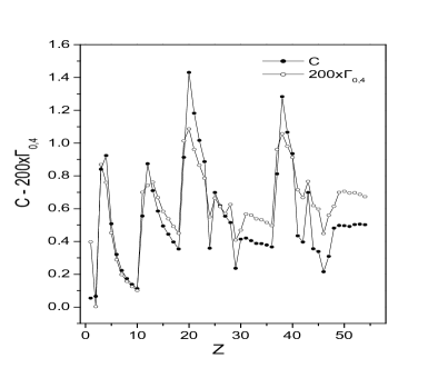
Figure 2: Comparison of C(Z) and 200$\times\Gamma_{0,4}(Z)$

Several cases for both $\alpha$ and $\beta$ non-negative are shown in Fig. 2 of Ref. [4], where $\Gamma_{\alpha,\beta}$ is shown as a function of $\Delta$. In our previous work [8] we obtained $\Delta=S/S_{\rm max}$ or $\Omega=1-\Delta$ as a function of $Z$ and plotted the dependence of $\Gamma_{\alpha,\beta}$ on the atomic number $Z$.

We employed $S_{{\rm max}}$ according to rigorous inequalities holding to atoms [26, 8], which hold for other systems as well (nuclei, atomic clusters and atoms in a trap–bosons) as verified in [14, 27]. These inequalities are

$$S_{r\,{\rm min}} \leq S_{r} \leq S_{r\,{\rm max}},$$ (15)

$$S_{k\,{\rm min}} \leq S_{k} \leq S_{k\,{\rm max}},$$ (16)

$$S_{\rm min} \leq S \leq S_{\rm max}.$$ (17)

The lower and the upper limits can be written, for density distributions normalized to one

$$S_{r\,{\rm min}} = \frac{3}{2}\,(1+\ln{\pi})-\frac{3}{2}\,\ln{\left(\frac{4}{3}\,T\right)},$$

$$S_{r\,{\rm max}} = \frac{3}{2}\,(1+\ln{\pi})+\frac{3}{2}\,\ln{\left(\frac{2}{3}\,\langle r^{2}\rangle\right)},$$ (18)

$$S_{k\,{\rm min}} = \frac{3}{2}\,(1+\ln{\pi})-\frac{3}{2}\,\ln{\left(\frac{2}{3}\,\langle r^{2}\rangle\right)},$$

$$S_{k\,{\rm max}} = \frac{3}{2}\,(1+\ln{\pi})+\frac{3}{2}\,\ln{\left(\frac{4}{3}\,T\right)},$$ (19)

$$S_{{\rm min}} = 3\,(1+\ln{\pi}),$$

$$S_{{\rm max}} = 3\,(1+\ln{\pi})+\frac{3}{2}\,\ln{\left(\frac{8}{9}\,\langle r^{2}\rangle\,T\right)},$$ (20)

where $\langle r^{2}\rangle$ is the mean square radius and $T$ is the kinetic energy. We employ in (12) $S_{\rm max}$ according to relation (20).

As an alternative, we may use instead of $\Gamma_{\alpha,\beta}$ the following statistical measure of complexity $C$ due to L$\acute{\textrm{o}}$pez-Ruiz, Mancini and Calbet [5] defined as

$$C=S\cdot D,$$ (21)

where $S$ denotes the information content stored in the system (in our case the information entropy sum $S=S_{r}+S_{k}$) and $D$ is the disequilibrium of the system i.e. the distance from its actual state to equilibrium [6, 7] defined for a discrete probability distribution $\{p_{i}\}$ as follows [6]

$$D(\{p_{i}\})=\sum_{i=1}^{N}\left(p_{i}-\frac{1}{N}\right)^{2},\quad\mbox{where}\,\,p_{i}\geq 0\,\,\mbox{and}\,\,\sum_{i=1}^{N}p_{i}=1.$$ (22)

$D$ is the quadratic distance of the actual probability distribution $\{p_{i}\}$ to equiprobability. In the continuous case, the rectangular function $\rho(x)=\frac{1}{2L}$, where $-L<x<L$, is the natural extension of the equiprobability distribution of the discrete case. Thus the disequilibrium could be defined as

$$D^{*}=\int_{-L}^{L}\left(\rho(x)-\frac{1}{2L}\right)^{2}\,dx=\int_{-L}^{L}\rho(x)^{2}\,dx-\frac{1}{2L}.$$ (23)

If we redefine $D$ omitting the constant adding term in $D^{*}$ (which is very small for large $L$), the disequilibrium reads now

$$D(\rho(x))=\int_{-L}^{L}\rho(x)^{2}\,dx,$$ (24)

where $D$ is positive for every distribution and minimal for the rectangular function which represents the equipartition. For large values of $L$ ($L\rightarrow\infty$) relation (24) gives

$$D=\int\rho^{2}(x)\,dx.$$ (25)

Another derivation of the formula (25) for continuous $\rho(x)$ can be found in Section 3 of [28] by using the Rényi generalized entropy

$$I_{q}=\frac{1}{1-q}\,\log\left({\sum_{i=1}^{N}p_{i}^{q}}\right),$$ (26)

where $q$ is an index running over all the integer values.

According to [5, 6, 7] $S$ and $D$ are the two basic ingredients for calculating complexity. In our 3-dimensional case, we employ instead of (25) the formula

$$D=E_{r}\cdot E_{k},$$ (27)

where $E_{r}$, $E_{k}$ are defined in (9), (10). Relation (27) extends the definition of measure of disequilibrium of the system according to LMC, to our case, where we are interested jointly in position- and momentum-spaces. It turns out that LMC definition of disequilibrium $D$ (25) is identical to Onicescu’s formula (7) for the information energy $E$. In fact, inspired by the work of L$\acute{\textrm{o}}$pez-Ruiz, Mancini and Calbet, a new interpretation of Onicescu information energy may be proposed i.e. it represents the disequilibrium of the system or distance from equilibrium. Additionally in our case something new is introduced, that is the effect of a delicate balance between conjugate spaces, reflected in the sum $S=S_{r}+S_{k}$ and the product $D=E_{r}\cdot E_{k}$. Both $S$ and $D$ are dimensionless.

3 Numerical results and discussion

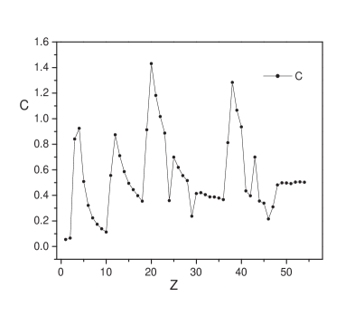
Figure 1: The LMC measure of complexity $C$ as function of the atomic number $Z$ of atoms.

The dependence of $\Gamma_{\alpha,\beta}$ on $Z$ for atoms has been calculated recently in [8]. In the present letter we calculate $C(Z)$ employing the same RHF wave functions in the same region $1<Z\leq 54$, for the sake of comparison. Our results are shown in Fig. 1 and Fig. 2. We compare them with $\Gamma_{\alpha,\beta}(Z)$ shown in Fig. 3 of [8] for $(\alpha,\beta)=(1,1),(1,1/4),(1/4,0),(0,4)$. In all (six) cases we observe that the measures of complexity show local minima at closed shells atoms, namely for $Z$=10 (Ne), 18 (Ar), 36 (Kr). The physical meaning of that behavior is that the electron density for those atoms is the most compact one compared to neighboring atoms. The local maxima can be interpreted as being far from the most compact distribution (low ionization potential systems). This does not contradict common sense and satisfies our intuition. There are also local minima for $Z$=24 (Cr), 29 (Cu), 42 (Mo). Those minima are due to a specific change of the arrangement of electrons in shells. For example, going from $Z$=24 (Cr) with electron configuration [Ar]$4\textrm{s}^{1}3\textrm{d}^{5}$ to the next atom $Z$=25 (Mn), with configuration [Ar]$4\textrm{s}^{2}3\textrm{d}^{5}$, it is seen that one electron is added in an s-orbital (highest). The situation is similar for $Z$=29 (Cu) and $Z$=42 (Mo). The local minimum for $Z=46$ (Pd) is due to the fact that Pd has a $4\textrm{d}^{10}$ electron configuration with extra stability of electron density. It has no $5\textrm{s}$ electron, unlike the neighboring atoms. There are also fluctuations of the complexity measures within particular subshells. This behavior can be understood in terms of screening effects within the subshell. The question naturally arises if the values of complexity correlate with properties of atoms in the periodic table. An example is the correlation of Onicescu information content $O$ with the ionization potential (Fig. 4 of [8]). A more detailed/systematic study is needed, which is beyond the scope of the present report.

Our calculations in [8] show a dependence of complexity on the indices of disorder $\alpha$ and order $\beta$. In [8], we made a general comment that there are fluctuations of complexity around an average value and atoms cannot grow in complexity as $Z$ increases. The second part of our comment needs to be modified. Various values of ($\alpha$,$\beta$) lead to different trends of $\Gamma_{\alpha,\beta}(Z)$ i.e. increasing, decreasing or approximately constant. In addition, in the present Letter we compare $C(Z)$ with $\Gamma_{\alpha,\beta}(Z)$ and we find a significant overall similarity between the curves $\Gamma_{0,4}(Z)$ and $C(Z)$ by plotting $C(Z)$ and $200\times\Gamma_{0,4}(Z)$ in the same Fig. (2). The numerical values are different but a high degree of similarity is obvious by simple inspection. There is also the same succession of local maxima and minima at the same values of $Z$. Less striking similarities are observed for other values of ($\alpha,\beta$) as well, e.g. $\Gamma_{1,1}(Z)$ and $C(Z)$.

Concluding, the behavior of SDL complexity depends on the values of the parameters $\alpha$ and $\beta$. The statistical measure LMC displays an increasing trend as $Z$ increases. An effort to connect the aforementioned measures, implies that LMC measure corresponds to SDL when the magnitude of disorder $\alpha\simeq 0$ and of order $\beta\simeq 4$. In other words, if one insists that SDL and LMC behave similarly as functions of $Z$, then we can conclude that complexity shows an overall increasing behavior with $Z$. Their correlation gives for atoms the strength of disorder $a\simeq 0$ and order $\beta\simeq 4$.

A final comment seems appropriate: An analytical comparison of the similarity of $\Gamma_{\alpha,\beta}(Z)$ and $C(Z)$ is not trivial. Combining equations (12) and (13) we find for the SDL measure

$$\Gamma_{\alpha,\beta}(Z)=\left(\frac{S}{S_{{\rm max}}}\right)^{\alpha}\left(1-\frac{S}{S_{{\rm max}}}\right)^{\beta},$$ (28)

while for the LMC one has

$$C=S\cdot\left(E_{r}E_{k}\right).$$ (29)

$S$ and $S_{{\rm max}}$ depend on $Z$ as follows

$$S(Z)=S_{r}(Z)+S_{k}(Z)=6.257+1.069\,\ln{Z}$$ (30)

(almost exact fitted expression) [29, 8], while

$$S_{{\rm max}}(Z)=S_{r\,{\rm max}}(Z)+S_{k\,{\rm max}}(Z)=7.335+1.658\,\ln{Z}$$ (31)

(a rough approximation). We mention that $S_{r}$, $S_{k}$, $E_{r}$, $E_{k}$ are known but different functionals of $\rho(\textbf{r})$ and $n(\textbf{k})$ according to relations (1), (2) and (9), (10) respectively. It is noted that our numerical calculations were carried out with exact values of $S_{r}$, $S_{k}$, $E_{r}$, $E_{k}$, while our fitted expressions for $S(Z)$, $S_{\textrm{max}}(Z)$ are presented in order to help the reader to appreciate approximately the trend of $\Gamma_{\alpha,\beta}(Z)$ and $C(Z)$.

4 Comments on the validity of SDL and LMC measures

Complexity is a multi-faceted and context dependent concept, difficult to be quantified. It is extremely difficult at present to define complexity under all possible circumstances. Instead, one can choose a pragmatic approach and use as a starting point definitions of complexity found in the literature and attempt to evolve the existing framework. Thus, we have chosen the simple SDL measure and the statistical LMC one, which are relatively easy to compute. The question naturally arises if the above measures do represent the concept of complexity as expected from semantics, intuition or other general criteria. SDL and LMC measures have also been criticized in several aspects [9, 10, 11], some of them are the following:

1. All systems with the same disorder $\Delta$ have the same $\Gamma_{\alpha,\beta}$ i.e. the function $\Gamma_{\alpha,\beta}(\Delta)$ is universal.

2. Landsberg’s definition of disorder $\Delta=S/S_{\rm max}$ does not describe properly and does not capture the system’s structure, pattern, organization, or symmetries.

3. The calculation in [4] of $\Gamma_{11}$ for equilibrium Ising systems is not clear.

In our previous and present work we use ground state electronic densities of atoms to evaluate $\Gamma_{\alpha,\beta}(Z)$ and $C(Z)$. At present it is not possible to answer semantic or sophisticated questions as the ones raised in [9, 10, 11] and described above. One cannot claim that SDL measure is the measure of complexity but it is a simple measure, indicating that it can be used as a starting point. To our knowledge, there are no other studies of complexity in quantum systems as functions of the number of particles.

The definition of $\Gamma_{\alpha,\beta}$ is based on Landsberg’s disorder $\Delta$ in terms of information measures $S$, $S_{\rm max}$ available as functions of $N$. By definition $\Omega$ and $\Delta$ are related by $\Omega+\Delta=1$. An alternative approach where $\Delta$ and $\Omega$ should be considered independent of each other, is an open one. Before considering such an extension, we calculate $\Gamma_{\alpha,\beta}(N)$ given in (28), where $S$ and $S_{\rm max}$ show different non-trivial dependence on $N$. In this sense the universality of $\Gamma_{\alpha,\beta}(\Delta)$ is modified: $\Gamma_{\alpha,\beta}(N)$ depends on the quantum system under consideration, i.e. atoms [8], nuclei, atomic clusters e.t.c. (work in progress). Instead of varying the number of particles $N$, one could keep it constant, and study the effect on complexity of other parameters of the system. A welcome property of a definition of complexity supporting its validity might be the following: If one complicates the system by varying some of its parameters, and this leads to an increase of the adopted measure of complexity, then one could argue that this measure describes the complexity of the system properly.

There have been several criticisms regarding the LMC measure of complexity in the sense that it does not deserve the adjective statistical, it is not a general measure that quantifies structure and it is not an extensive quantity [9]. Analogous arguments with SDL could be given to support the use of LMC as a first working prototype of complexity to be modified by more sophisticated models. In [11] various properties of the SDL measure are examined and a modification is attempted to remove its insensitivity to system differences. However in our present (quantum) case of atoms, by employing solely electron density distributions, it is difficult to check these ideas.

In addition, the similarity of the qualitative behavior of $\Gamma_{\alpha,\beta}(Z)$ and $C(Z)$ for atoms used as a case study (although they obey different definitions) is interesting. It shows that both measures share some common traits and correlate strongly with the periodicity of the elements in the periodic table. An important issue is the question if $\Gamma$ and $C$ are true measures of complexity (structure, pattern etc) or are just functionals of electron densities. Further research is needed to clarify their region of validity and applicability as measures of complexity.

Information entropy is an extensive quantity. The question arises if $\Gamma_{\alpha,\beta}$ and $C$ are extensive or intensive quantities, what is their thermodynamic limit, their behavior at the boundaries (large or small order), their properties under scaling transformations e.t.c. For example, it is stated in [10] that $C$ is neither an intensive nor an extensive thermodynamic variable and it vanishes exponentially in the thermodynamic limit, for all one-dimensional, finite-range systems. However, in a broader context, $\Gamma_{\alpha,\beta}$ and $C$ can serve as indicators of complexity, based on a probabilistic description. In some cases it can be applied in a setting wider or different than thermodynamics. Such a case, is the calculation of $C$ for various shapes of probability distributions $\rho(x)$ in [6], i.e. the rectangular, the isosceles–triangle, the Gaussian and the exponential probability distributions which are classified according to the corresponding values of $C$.

Another case is the present work, where $\Gamma_{\alpha,\beta}$ and $C$ are estimated for the ground state electron densities, $\rho(r)$ and $n(k)$, of a quantum system (atom) at zero temperature. To our knowledge, such an application is done for the first time for a quantum system, and deserves more detailed investigation (e.g. for excited states). It is true that there are certain shortcomings of $\Gamma_{\alpha,\beta}$ and $C$ for various cases in statistical mechanics. In quantum systems further investigation is needed. Our title ”$\ldots$Atoms as a testbed” describes well our aim.

5 Acknowledgments

The work of K. Ch. Chatzisavvas was supported by Herakleitos Research Scholarships (21866) of $\textrm{E}\Pi\textrm{EAEK}$ and the European Union. The work of Ch. C. Moustakidis was supported by Pythagoras II Research project (80861) of $\textrm{E}\Pi\textrm{EAEK}$ and the European Union.

References

- [1] N. Goldenfeld and L. Kadanoff, Science 284 87 (1999).
- [2] A. N. Kolmogorov, Probl. Inf. Transm. 1, 3 (1965).
- [3] G. Chaitin, J. ACM 13 547 (1966).
- [4] J. S. Shiner, M. Davison, and P. T. Landsberg, Phys. Rev. E 59, 1459 (1999).
- [5] R. Lpez-Ruiz, H. L. Mancini, and X. Calbet, Phys. Lett. A 209, 321 (1995).
- [6] R. G. Catalan, J. Garay, and R. Lopez-Ruiz, Phys. Rev. E 66, 011102 (2002).
- [7] J. R. Snchez and R. Lpez-Ruiz, Physica A 355, 633 (2005).
- [8] K. Ch. Chatzisavvas, Ch. C. Moustakidis, and C. P. Panos, J. Chem. Phys. 123, 174111 (2005).
- [9] J. Crutchfield, D. P. Feldman, and C. R. Shalizi, Phys. Rev. E 62, 2996 (2000).
- [10] D. P. Feldman and J. Crutchfield, Phys. Lett. A 238, 244 (1998).
- [11] R. Stoop, N. Stoop, A. Kern, and W-H Steeb, J. Stat. Mech.: Theory and Experiment, 11009 (2005).
- [12] C. P. Panos and S. E. Massen, Int. J. Mod. Phys. E 6, 497 (1997).
- [13] S. E. Massen and C. P. Panos, Phys. Lett. A 246, 530 (1998).
- [14] S. E. Massen and C. P. Panos, Phys. Lett. A 280, 65 (2001).
- [15] G. A. Lalazissis, S. E. Massen, C. P. Panos, and S. S. Dimitrova, Int. J. Mod. Phys. E 7, 485 (1998).
- [16] Ch. C. Moustakidis, S. E. Massen, C. P. Panos, M. E. Grypeos, and A. N. Antonov, Phys. Rev. C 64, 014314 (2001).
- [17] C. P. Panos, S. E. Massen, and C. G. Koutroulos, Phys. Rev. C 63, 064307 (2001).
- [18] C. P. Panos, Phys. Lett. A 289, 287 (2001).
- [19] S. E. Massen, Phys. Rev. C 67, 014314 (2003).
- [20] Ch. C. Moustakidis and S. E. Massen, Phys. Rev. B 71, 045102 (2003).
- [21] S. E. Massen, Ch. C. Moustakidis, and C. P. Panos, Focus on Boson Research (Nova Publishers, New York, 2005), p. 115.
- [22] C. F. Bunge, J. A. Barrientos, and A. V. Bunge, At. Data Nucl. Data Tables 53, 113 (1993).
- [23] T. Koga, K. Kanayama, S. Watanabe, T. Imai, and A. J. Thakkar, Chem. Acc. 104, 411 (2002).
- [24] O. Onicescu, CR Acad. Sci. Paris A 263, 25 (1966).
- [25] P. T. Landsberg, Phys. Lett. A 102, 171 (1984).
- [26] S. R. Gadre and R. D. Bendale, Phys. Rev. A 36, 1932 (1987).
- [27] S. E. Massen, Ch. C. Moustakidis, and C. P. Panos, Phys. Lett. A 299, 131 (2002).
- [28] R. Lpez-Ruiz, Biophys. Chem. 115, 215 (2005).
- [29] S. R. Gadre, S. B. Sears, S. J. Chakravorty, and R. D. Bendale, Phys. Rev. A 32, 2602 (1985).