The Quantum Gate Design Metric

Abstract

What is the time-optimal way of realizing quantum operations? Here, we show how important instances of this problem can be related to the study of shortest paths on the surface of a sphere under a special metric. Specifically, we provide an efficient synthesis of a controlled NOT (CNOT) gate between qubits (spins $\frac{1}{2}$) coupled indirectly via Ising-type couplings to a third spin. Our implementation of the CNOT gate is more than twice as fast as conventional approaches. The pulse sequences for efficient manipulation of our coupled spin system are obtained by explicit computation of geodesics on a sphere under the special metric. These methods are also used for the efficient synthesis of indirect couplings and of the Toffoli gate. We provide experimental realizations of the presented methods on a linear three-spin chain with Ising couplings.

1 Introduction

Quantum computation promises solution to problems that are hard to solve by classical computers [1, 2]. The efficient construction of quantum circuits that can solve interesting tasks is a fundamental challenge in the field. Efficient construction of quantum circuits also reduces decoherence losses in physical implementations of quantum algorithms by reducing interaction time with the environment. Therefore, finding time-optimal ways to synthesize unitary transformations from available physical resources is a problem of both fundamental and practical interest in quantum information processing. It has received significant attention, and time-optimal control of two coupled qubits [4, 5, 6, 7] is now well understood. Recently, this problem has also been studied in the context of linearly coupled three-qubit topologies [8], where significant savings in implementation time of trilinear Hamiltonians were demonstrated over conventional methods. However, the complexity of the general problem of time optimal control of multiple qubit topologies is only beginning to be appreciated. The scope of these issues extends to broader areas of coherent spectroscopy and coherent control, where it is desirable to find time optimal ways to steer quantum dynamics between points of interest to minimize losses due to couplings to the environment [9, 10].

One approach of effectively tackling this task is to map the problem of efficient synthesis of unitary transformations to geometrical question of finding shortest paths on the group of unitary transformations under a modified metric [4, 8, 3]. The optimal time variation of the Hamiltonian of the quantum system that produces the desired transformation is obtained by explicit computation of these geodesics. The metric enforces the constraints on the quantum dynamics that arise because only limited Hamiltonians can be realized. Such analogies between optimization problems related to steering dynamical systems with constraints and geometry have been well explored in areas of control theory [11, 12] and sub-Riemannian geometry [13]. In this paper, we study in detail the metric and the geodesics that arise from the problem of efficient synthesis of couplings and quantum gates between indirectly coupled qubits in quantum information processing.

Synthesizing interactions between qubits that are indirectly coupled through intermediate qubits is a typical scenario in many practical implementations of quantum information processing and coherent spectroscopy. Examples include implementing two-qubit gates between distant spins on a spin chain [14, 15] or using an electron spin to mediate couplings between two nuclear spins [16]. Multidimensional NMR experiments require synthesis of couplings between indirectly coupled qubits in order to generate high resolution spectral information [17]. The synthesis of two-qubit gates between indirectly coupled qubits tends to be expensive in terms of time for their implementation. This is because such gates are conventionally constructed by concatenating two-qubit operations on directly coupled spins. Lengthy implementations lead to relaxation losses and poor fidelity of the gates. In this paper, we develop methods for efficiently manipulating indirectly coupled qubits. In particular, we study the problem of efficient synthesis of couplings and CNOT gate between indirectly coupled spins and demonstrate significant improvement in implementation time over conventional methods. We also show how these methods can be used for efficient synthesis of other quantum logic gates like for example, a Toffoli gate [18, 19, 20] on a three-qubit topology, with qubits $1$ and $3$ indirectly coupled through coupling to qubit $2$. Experimental implementations of the main ideas are demonstrated for a linear three-spin chain with Ising couplings in solution state NMR.

2 Theory

A geodesic is the shortest path between two points in a curved space. Under the standard Euclidean metric $(dx)^{2}+(dy)^{2}+(dz)^{2}$, the geodesics connecting any two points in a plane are straight lines and geodesics on a sphere are segments of great circles. In this paper, we study the geodesics on a sphere under the metric $g=\frac{(dx)^{2}+(dz)^{2}}{y^{2}}$ (note on the unit sphere $y^{2}=1-x^{2}-z^{2}$). The solid curve in Fig. 1 depicts the shortest path connecting the north pole $(1,0,0)$ to a point $(0,\cos\phi,\sin\phi)$, under the metric $g$. The dashed curve is the geodesic under the standard metric and represents a segment of a great circle. For $\phi=\frac{\pi}{4}$, the length $L$ of the geodesic under $g$ is $0.627\pi$ (as opposed to $\frac{\pi}{2}$ under standard metric). We call this metric $g$, the quantum gate design metric. If $w$ represents the complex number $w=x+iz$, then the quantum gate design metric can be written an

$$g=\frac{|dw|^{2}}{1-|w|^{2}}.$$

It has marked similarity to the Poincare metric $\frac{|dw|^{2}}{(1-|w|^{2})^{2}}$, in Hyperbolic geometry [21], defined on the unit disc.

We show how problems of efficiently steering quantum dynamics of coupled qubits can be mapped to the study of shortest paths under the metric $g$. Computing geodesics under $g$ helps us to develop techniques for efficient synthesis of transformations in the 63 dimensional space of (special) unitary operators on three coupled qubits.

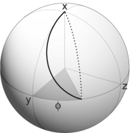
Figure 1: The solid curve in Fig. 1 depicts the shortest path connecting the north pole $(1,0,0)$ to a point $(0,\cos\phi,\sin\phi)$, under the metric $g$. The dashed curve is the geodesic under the standard metric and represents a segment of a great circle.

We consider a linear Ising chain, consisting of three coupled qubits (spins 1/2) with coupling constants $J_{12}=J_{23}=J$ and $J_{13}=0$ (see Fig. 2 A). The coupling Hamiltonian between the qubits is given by [17]

$${\cal H}_{c}=2\pi J(I_{1z}I_{2z}+I_{2z}I_{3z}).$$

The spin system is controlled by local unitary operations on individual qubits, which we assume take negligible time compared to the evolution of couplings [4]. The strength of couplings limits the time it takes to synthesize quantum logical gates between coupled qubits. We seek to find the optimal way to perform local control on qubits in the presence of evolution of couplings to perform fastest possible synthesis of quantum logic gates. For directly coupled qubits, this problem has been solved. For example, a CNOT(1,2) gate which inverts spin 2 conditioned on the state of spin 1 requires a minimum of $0.5\ J^{-1}$ [4]. Here, we focus on the problem of synthesizing the CNOT(1,3) gate between indirectly coupled spins. Fig. 2 B shows the energy level diagram for the CNOT(1,3)operation, where the state of qubit $3$ is inverted if qubit $1$ is in a lower energy state, i.e., in state $1$. In the literature, various constructions of CNOT(1,3) have been considered with durations ranging from 3.5 $J^{-1}$ to 2.5 $J^{-1}$ [22]. The main result of this paper is that the $CNOT(1,3)$ gate can be realized in only $\frac{2L}{\pi J}$ units of time, where $L$ is the length of the geodesic under the metric $g$ for $\phi=\frac{\pi}{4}$ as depicted in Fig. 1. This is twice as fast as the best known conventional approach. The new pulse sequence for CNOT(1,3) is based on the sequence element shown in Fig. 3 A.

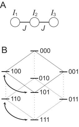
Figure 2: Fig. 2 A shows the coupling topology where the first qubit ($I_{1}$) and third qubit ($I_{3}$) are coupled only indirectly via the second qubit ($I_{2}$) with coupling constants $J_{12}=J_{23}=J$. Fig. 2 B shows a schematic energy level diagram for the spin system in a static magnetic field in the $z$ direction, which determines the quantization axis. $1$ and $0$ are low and high energy eigenstates of the angular momentum operator along the $z$ direction. The effect of the unitary transformation CNOT(1, 3) is shown in the figure.

The main ideas for discovering efficient new pulse sequence are as follows. The unitary propagator for a CNOT gate is

$$CNOT(1,3)=\exp\{-{\rm i}{\pi\over 2}\ (2I_{1z}I_{3x}-I_{1z}-I_{3x}+{1\over 2}{\bf 1})\},$$

where ${\bf 1}$ is the identity operator and $I_{k\alpha}$ is 1/2 times the Pauli-spin operator on qubit $k$ with $\alpha\in\{x,y,z\}$ [17]. Since we assume that local operations take negligible time, we consider the synthesis of the unitary operator

$${\cal U}_{13}^{s}=\exp\{-{\rm i}\frac{\pi}{2}(I_{1z}+I_{3z}+2I_{1z}I_{3z})\},$$

which is locally equivalent to $CNOT(1,3)$ but symmetric in qubits 1 and 3.

For synthesizing ${\cal U}_{13}^{s}$, we seek to engineer a time varying Hamiltonian that transforms the various quantum states in the same way as ${\cal U}_{13}^{s}$ does. The unitary transformation ${\cal U}_{13}^{s}$ transforms the operators $I_{1\alpha}$ and $I_{3\alpha}$, with $\alpha\in\{x,y\}$ to $-2I_{1\alpha}I_{3z}$ and $-2I_{1z}I_{3\alpha}$ respectively. Since ${\cal U}_{13}^{s}$ treats the operators $I_{1x,1y}$ and $I_{3x,3y}$ symmetrically, we seek to construct the propagator ${\cal U}_{13}^{s}$ by a time varying Hamiltonian that only involves the evolution of Hamiltonian ${\cal H}_{c}$ and single qubit operations on the second spin. The advantage of restricting to only these two control actions is that it is then sufficient to engineer a pulse sequence for steering just the initial state $I_{1x}$ to its target operator $-2I_{1x}I_{3z}$. Other operators in the space $\{I_{1\alpha},I_{3\beta},2I_{1\alpha}I_{3\beta}\}$ are then constrained to evolve to their respective targets (as determined by the action of ${\cal U}_{13}^{s}$). Our approach can be broken down into the following steps:

(I) In a first step, the problem of efficient transfer of $I_{1x}$ to $-2I_{1x}I_{3z}$ in the 63 dimensional operator space of three qubits is reduced to a problem in the six-dimensional operator space $\cal{S}$, spanned by the set of operators $I_{1x}$ , $2I_{1y}I_{2z}$, $2I_{1y}I_{2x}$, $4I_{1y}I_{2y}I_{3z}$, $4I_{1y}I_{2z}I_{3z}$, and $2I_{1x}I_{3z}$ (The numerical factors of $2$ and $4$ simplifies the commutation relations among the operators). The subspace $\cal{S}$ is the lowest dimensional subspace in which the initial state $I_{1x}$ and the target state $-2I_{1x}I_{3z}$ are coupled by ${\cal H}_{c}$ and the single qubit operations on the second spin.

(II) In a second step, the six-dimensional problem is decomposed into two independent (but equivalent) four-dimensional time-optimal control problems.

(III) Finally, it is shown that the solution of these time optimal control problems reduces to computing shortest paths on a sphere under the modified metric $g$.

In step (I), any operator in the six-dimensional subspace $\cal{S}$ of the 63-dimensional operator space is represented by the coordinates $\ x=(x_{1},x_{2},x_{3},x_{4},x_{5},x_{6})$, where the coordinates are given by the following six expectation values: $x_{1}=\langle I_{1x}\rangle$, $x_{2}=\langle 2I_{1y}I_{2z}\rangle$, $x_{3}=\langle 2I_{1y}I_{2x}\rangle$, $x_{4}=\langle 4I_{1y}I_{2y}I_{3z}\rangle$, $x_{5}=\langle 4I_{1y}I_{2z}I_{3z}\rangle$, and $x_{6}=-\langle 2I_{1x}I_{3z}\rangle$. In the presence of the coupling ${\cal H}_{c}$, a rotation of the second qubit around the $y$ axes (effected by a rf-Hamiltonian ${\cal H}_{a}=u_{a}(t)\pi JI_{2y}$) couples the first four components $x_{A}^{\prime}=(x_{1},x_{2},x_{3},x_{4})$ of the vector $x$. In the presence of ${\cal H}_{c}$, a rotation around the $x$ axes (effected by a rf-Hamiltonian ${\cal H}_{b}=u_{b}(t)\pi JI_{2x}$) mixes the last four components $x_{B}^{\prime}=(x_{3},x_{4},x_{5},x_{6})$ of the vector $x$. Under $x$ or $y$ pulses applied to the second qubit in the presence of ${\cal H}_{c}$, the equations of motion for $x_{A}$ and $x_{B}$ have the same form:

$$\frac{dx_{A,B}}{dt}=\pi J\ \left(\begin{array}[]{cccc}0&-1&0&0\\ 1&0&-u_{A,B}&0\\ 0&u_{A,B}&0&-1\\ 0&0&1&0\end{array}\right)\ x_{A,B}.$$ (1)

Since evolution of $x_{A}$ and $x_{B}$ is equivalent, it motivates the following sequence of transformations that treats the two systems symmetrically and steers $I_{1x}$ (corresponding to $x_{A}=(1,0,0,0)$) to $-2I_{1x}I_{3z}$ (corresponding to $x_{B}=(0,0,0,1)$):

(a) Transformation from $(1,0,0,0)$  to  $(0,x_{2}^{\prime},x_{3}^{\prime},\frac{1}{\sqrt{2}})$ in subsystem A with $\sqrt{x_{2}^{\prime 2}+x_{3}^{\prime 2}}=\frac{1}{\sqrt{2}}$.

(b) Transformation from $(0,x_{2}^{\prime},x_{3}^{\prime},\frac{1}{\sqrt{2}})$  to  $(0,0,\frac{1}{\sqrt{2}},\frac{1}{\sqrt{2}})$ in subsystem A (corresponding to $(\frac{1}{\sqrt{2}},\frac{1}{\sqrt{2}},0,0)$ in subsystem B).

(c) Transformation from $(\frac{1}{\sqrt{2}},\frac{1}{\sqrt{2}},0,0)$ to $(\frac{1}{\sqrt{2}},x_{3}^{\prime},x_{2}^{\prime},0)$ in subsystem B.

(d) Transformation from $(\frac{1}{\sqrt{2}},x_{3}^{\prime},x_{2}^{\prime},0)$ to $(0,0,0,1)$ in subsystem B.

The transformations (b) and (c) represent fast y and x rotations of the second spin respectively and are realized by hard pulses which take a negligible amount of time: Transformation (b) is accomplished by hard $\theta_{y}$ pulse applied to the second qubit, i.e. a pulse with flip angle $\theta$ (where $\tan\theta=x_{2}^{\prime}/x_{3}^{\prime}$) and phase $y$. Similarly, transformation (c) can be accomplished by hard $\theta_{x}$ pulse applied to the second qubit. Because of the symmetry of the two subsystems A and B, the transformations (a) and (d) are equivalent and take the same amount of time with (d) being the time-reversed transformation of (a) and $x_{5}$ and $x_{6}$ replacing $x_{2}$ and $x_{1}$ respectively. Hence the problem of finding the fastest transformations (a)-(d), reduces to a time-optimal control problem in the four-dimensional subspace A, asking for the choice of $u_{A}(t)$ that achieves transfer (a) in the minimum time.

In step (III), this optimal control problem is reduced to the shortest path problem on a sphere (under metric $g$) described in the beginning of the section (see Fig. 1). The key ideas are as follows. Let $x(t)=x_{1}(t)$, $y(t)=\sqrt{x_{2}^{2}(t)+x_{3}^{2}(t)}$ and $z(t)=x_{4}(t)$. Since $u_{A}(t)$ can be made large, we can control the angle $\tan\theta(t)=\frac{x_{2}(t)}{x_{3}(t)}$ arbitrarily fast. With the new variables $(x(t),y(t),z(t))$, equation (1) reduces to

$$\frac{d}{dt}\left[\begin{array}[]{c}x\\ y\\ z\end{array}\right]=\pi J\left[\begin{array}[]{cccc}0&-\sin\theta(t)&0\\ \sin\theta(t)&0&-\cos\theta(t)\\ 0&\cos\theta(t)&0\end{array}\right]\left[\begin{array}[]{c}x\\ y\\ z\end{array}\right].$$ (2)

In this system, the goal of achieving the fastest transformation (a) corresponds to finding the optimal angle $\theta(t)$ such that $(1,0,0)$ is steered to $(0,\frac{1}{\sqrt{2}},\frac{1}{\sqrt{2}})$ in the minimum time. The time of transfer $\tau$ can be written as $\int_{0}^{\tau}\sqrt{\sin^{2}\theta(t)+\cos^{2}\theta(t)}\ dt$. Substituting for $\sin\theta(t)$ and $\cos\theta(t)$ from (2), this reduces to

$$\frac{1}{\pi J}\underbrace{\int\sqrt{\frac{(\dot{x})^{2}+(\dot{z})^{2}}{y^{2}}}dt}_{L},$$

where $L$ is the length of the trajectory connecting $(1,0,0)$ to $(0,\frac{1}{\sqrt{2}},\frac{1}{\sqrt{2}})$. Thus minimizing $\tau$ amounts to computing the geodesic under the metric $g$. The Euler-Lagrange equations for the geodesic take the form $\frac{d}{dt}(\frac{\dot{x}}{y})=-(\pi J)^{-1}(\frac{\dot{z}}{y})$ and $\frac{d}{dt}(\frac{\dot{z}}{y})=(\pi J)^{-1}(\frac{\dot{x}}{y})$. For geodesics originating from $(1,0,0)$, this implies

$$\frac{\dot{x}}{y}=(\pi J)^{-1}\cos(ft);\ \ \frac{\dot{z}}{y}=(\pi J)^{-1}\sin(ft),$$

and $\theta(t)=ft$, for constant $f$ that depends of $\phi$. Now differentiating the expression $\frac{x_{2}}{x_{3}}(t)=\tan(ft)$ gives $u_{A}(t)=-\frac{f}{\pi J}+\frac{\dot{z}x-\dot{x}z}{y^{2}}$. The Euler-Lagrange equations imply that along geodesic curves, $\frac{\dot{z}x-\dot{x}z}{y^{2}}$ is constant, implying that in Eq. (1), time optimal $u_{A}(t)=u$ is constant. We now simply search numerically for this constant $u$ and the corresponding $\tau$ that will perform transformation (a) in system (1). From all feasible $(u,\tau)$ pairs, we choose the one with smallest $\tau$. This gives $\tau=0.627J^{-1}$ and $u_{A}(t)=u_{B}(t)=u=1.04$. Evolving (1) for time $\tau$ with $u=1.04$ results in $\theta(\tau)=\tan^{-1}\frac{x_{2}^{\prime}}{x_{3}^{\prime}}=0.5476$. The optimal flip angle for the transformations (a) and (d) is therefore $\theta=0.5476$. With this, the total unitary operator ${\cal U}_{13}^{g}$, corresponding to the transformations (a)-(d) can be written in the form

$${\cal U}_{13}^{g}={\Pi}_{x}\exp\{-{\rm i}\theta I_{2x}\}\exp\{-{\rm i}\theta I_{2y}\}{\Pi}_{y}$$ (3)

with ${\Pi}_{x,y}=\exp\{-{\rm i}\pi J\tau\ [2I_{1z}I_{2z}+2I_{2z}I_{3z}+uI_{2x,2y}]\}$. The pulse sequence for the implementation of ${\cal U}_{13}^{g}$ is evident from (3) and consists of a constant y pulse on spin $2$ of amplitude $\nu_{a}=uJ/2=0.52J$ for a duration of $\tau=0.627J^{-1}$ followed by a y pulse and then a x pulse each of flip angle $\theta=0.5476$ (corresponding to 31.4^∘) on spin 2, both of negligible duration. Finally, we apply a constant x pulse on spin 2 of duration $\tau=0.627J^{-1}$ and amplitude 0.52 $J$. The overall duration for the implementation of ${\cal U}_{13}^{g}$ is $T=2\tau=1.253J^{-1}$.

We now show that ${\cal U}_{13}^{g}$ is locally equivalent to ${\cal U}_{13}^{s}$ (and hence to CNOT(1,3)). Therefore CNOT(1,3) can also be implemented in a time $T=2\tau=1.253J^{-1}$. Let ${\cal I}_{1,3}$, denote the subspace spanned by operators $\{I_{1\alpha},I_{3\beta},I_{1\alpha}I_{3\beta}\}$ with independent $\alpha$, $\beta\in\{x,y,z\}$ and ${\cal I}_{2}$ denote the space spanned by operators $\{I_{2\alpha}\}$. It can be explicitly verified that by construction ${\cal U}_{13}^{g}$ maps ${\cal I}_{1,3}$ to itself and acts identically as ${\cal U}_{13}^{s}$. This constrains ${\cal U}_{13}^{g}$ to a local transformation on the space ${\cal I}_{1,3}\otimes{\cal I}_{2}$. We can therefore find local transformations $U^{loc}_{a}$, $U^{loc}_{b}$, and $U^{loc}_{c}$ such that

$$CNOT(1,3)=U^{loc}_{c}U^{loc}_{b}{\cal U}_{13}^{g}U^{loc}_{a}.$$

These local transformations are readily computed to equal $U^{loc}_{a}=\exp\{-{\rm i}{\pi\over 2}I_{3y}\}$, $U_{b}^{loc}=\exp\{{\rm i}(\pi-\theta)I_{2y}\}\exp\{{\rm i}(\pi-\theta)I_{2x}\}\exp\{{\rm i}\frac{\pi}{2}\ (I_{1z}+I_{3z})\}$, and $U^{loc}_{c}=\exp\{-{\rm i}{\pi\over 2}(I_{1z}-I_{3z})\}\exp\{-{\rm i}{\pi\over 2}I_{3x}\}$. Furthermore, the propagator

$${\cal U}_{13}=\exp\{-{\rm i}{\pi\over 2}\ (2I_{1z}I_{3z})\}=U^{loc}_{b}{\cal U}_{13}^{g},$$ (4)

representing a ${\pi\over 2}$ rotation under an effective 1-3 Ising coupling can also be generated in time $T=1.253J^{-1}$.

Figure 3: Efficient pulse sequences based on sub-Riemannian geodesics for the implementation of ${\cal U}_{13}=\exp\{-{\rm i}{\pi\over 2}\ 2I_{1z}I_{3z}\}$ (A), $\sqrt{{\cal U}_{13}}=\exp\{-{\rm i}{\pi\over 4}\ 2I_{1z}I_{3z}\}$ (B), simulating coupling evolution by angles ${\pi\over 2}$ (A) and ${\pi\over 4}$ (B) between indirectly coupled qubits, and of a Toffoli gate (C). Qubits $I_{1}$, $I_{2}$, and $I_{3}$ are assumed to be on resonance in their respective rotating frames. The unitary operator ${\cal U}_{13}$, which is locally equivalent to the CNOT(1,3) gate, is synthesized by sequence A in a total time $T^{\ast}_{C}=2\tau=1.253\ J^{-1}$. The amplitude of the weak pulses (represented by gray boxes) with a duration of $\tau=0.627\ J^{-1}$ is $\nu_{a}=uJ/2=0.52\ J$. The hard-pulse flip angles are $\theta=31.4^{\circ}$ and $\alpha=180^{\circ}-\theta=148.6^{\circ}$. Sequence B of total duration $(4+\sqrt{7})/4\ J^{-1}=1.66\ J^{-1}$ synthesizes the propagator $\sqrt{{\cal U}_{13}}$. The amplitude of the weak pulse (gray box) with a duration of $\sqrt{7}/4\ J^{-1}=0.661\ J^{-1}$ is $\nu_{w}=3J/\sqrt{7}=1.134\ J$. Pulse sequence C realizes the Toffoli gate in a total time $(6+\sqrt{7})/4\ J^{-1}=2.16\ J^{-1}$. The sequence is based on the sequence for $\sqrt{{\cal U}_{13}}$ and a weak pulse with the same amplitude and duration as in sequence B.

The methods developed above can also be used for efficient construction of trilinear propagators. This problem has been studied in detail in [8]. The main results of [8] become transparent in terms of geodesics under the metric $g$. Consider the propagator ${\cal U}_{zyz}(\kappa)=\exp\{-{\rm i}2\pi\kappa\ I_{1z}I_{2y}I_{3z}\}$. To synthesize this propagator, we again seek to efficiently steer the various states between points as they would transform under $U_{zyz}(\kappa)$. For example $I_{1x}$ is transferred to $I_{1x}\cos\kappa+\sin\kappa\ 4I_{1y}I_{2y}I_{3z}$. Consider again the four-dimensional operator space $A$ defined exactly as before. The goal now is to steer the initial vector $x_{A}$ from initial state $(1,0,0,0)$ to $(\cos\kappa,0,0,\sin\kappa)$ in Eq. (1). This in the transformed system Eq. (2), reduces to steering $(x,y,z)$ from $(1,0,0)$ to $(\cos\kappa,0,\sin\kappa)$. The geodesics for this problem have already been characterized. The length of the geodesic that maps $(1,0,0)$ to $(\cos\kappa,0,\sin\kappa)$ under the metric $g$ takes the form $L(\kappa)=\pi\frac{\sqrt{\kappa(4-\kappa)}}{2}$ and leads to a minimum time of $\tau(\kappa)$ of [8]

$$\tau(\kappa)=\frac{\sqrt{\kappa(4-\kappa)}}{2J}.$$ (5)

The time optimal $u_{A}(t)$ in Eq. 1 is again constant and the resulting unitary propagator is locally equivalent to ${\cal U}_{zyz}(\kappa)$. Since all trilinear propagators $U_{\alpha\beta\gamma}$ are locally equivalent, we get efficient ways of synthesizing all these propagators.

3 Discussion

We now compare the efficient synthesis of $CNOT(1,3)$ presented above with some conventional methods. The most simple approach (C1) to implement an indirect CNOT gate between spin $1$ and $3$ involves swapping the state of spins 1 and 2 followed by a $CNOT(2,3)$ and a final swap between 1 and 2, resulting in $CNOT(1,3)=SWAP(1,2)\ CNOT(2,3)\ SWAP(1,2)$. The minimum time for implementing CNOT gate between directly coupled spins 2 and 3 is 0.5$J^{-1}$ [4] and each SWAP operation takes 1.5$J^{-1}$ units of time, resulting in a total implementation time of 3.5$J^{-1}$ [22].

Since we assume that local operations take negligible time, the central step in synthesizing $CNOT(1,3)$ is the construction of the unitary operator ${\cal U}_{13}=\exp\{-{\rm i}\pi\ I_{1z}I_{3z}\}$. The standard method of synthesizing such an operator creates a trilinear propagator ${\cal U}_{zzy}=\exp\{-{\rm i}{\pi\over 2}\ 4I_{1z}I_{2z}I_{3y}\}$ and uses the following identity ${\cal U}_{13}=\exp\{-{\rm i}H_{1}\}{\cal U}_{zzy}\exp\{{\rm i}H_{1}\}$, and ${\cal U}_{zzy}=\exp\{-{\rm i}H_{2}\}\exp\{-{\rm i}{\pi\over 2}\ 2I_{1z}I_{2y}\}\exp\{{\rm i}H_{2}\}$, where $H_{1}={\pi\over 2}2I_{2z}I_{3x}$ and $H_{2}={\pi\over 2}2I_{2x}I_{3y}$. Overall, this takes 2.5$J^{-1}$ units of time [22], resulting in a realization (C2) of the $CNOT(1,3)$ gate that takes only 71.4% of the time required for the implementation (C1).

The time to synthesize $CNOT(1,3)$ can thus be shortened by reducing the time to synthesize the propagator ${\cal U}_{zzy}$. We can use a more efficient synthesis of these trilinear propagators discussed in [8] to further improve the efficiency of synthesis of $CNOT(1,3)$. Note

$${\cal U}_{zzy}=\exp\{{\rm i}{\pi\over 2}\ I_{2z}\}\exp\{-{\rm i}H_{3x}\}\exp\{-{\rm i}2H_{3y}\}\exp\{{\rm i}H_{3x}\},$$

where $H_{3\alpha}=\frac{\pi}{4}(2I_{1z}I_{2\alpha}+2I_{2\alpha}I_{3y})$, with $\alpha\in\{x,y,z\}$. This reduces the implementation time of ${\cal U}_{zzy}$ to $J^{-1}$ and of $CNOT(1,3)$ to 2$J^{-1}$ (C3). This time can be even further reduced by using the fact that the shortest time to produce the propagator ${\cal U}_{zzy}$ is given by $\sqrt{3}/(2J)$ [8] (see Eq. 5) and uses the identity

$${\cal U}_{zzy}=\exp\{{\rm i}{\pi\over 2}\ I_{2z}\}\exp\{-{\rm i}{{\sqrt{3}{\pi\over 2}}}\ (2I_{1z}I_{2x}+2I_{2x}I_{3y}+{2\over\sqrt{3}}I_{2z})\}\exp\{-{\rm i}{{3\pi}\over 2}I_{2z}\}.$$ (6)

This implementation then results in a total time of $(2+\sqrt{3})/(2J)=1.866/J$ (C4) for the $CNOT(1,3)$. The implementation (C5) proposed here is still significantly shorter than this. The implementation times under various strategies are summarized in Table 1.

Table 1: Duration $\tau_{c}$ of various implementations of $CNOT(1,3)$

pulse sequence	$\tau_{c}/J^{-1}$	relative duration
sequence 1 (C1)	3.5	100%
sequence 2 (C2)	2.5	71.4%
sequence 3 (C3)	2.0	57.1 %
sequence 4 (C4)	1.866	53.3 %
sequence 5 (C5)	1.253	38.8 %

We now show how efficient implementation of trilinear propagators can also be used for efficient construction of other quantum gates like a controlled controlled NOT (Toffoli) gate on spin $3$ conditioned on the state of spin $1$ and $2$ for the linear spin chain architecture. The decomposition given in [20] is based on four CNOT gates (requiring 0.5 $J^{-1}$ each) between directly coupled qubits and two CNOT gates between indirectly coupled qubits. Hence, using a SWAP-based implementation of the CNOT(1,3) gates (C1), each of which requires 3.5 $J^{-1}$, the total duration of the Toffoli gate would be 9 $J^{-1}$ (T1). With the most efficient implementation of CNOT(1,3) (C5), each of which requires 1.253 $J^{-1}$, the decomposition [20] has a total duration of about 4.5 $J^{-1}$ (T2). The Sleator-Weinfurter construction [19] of the Toffoli gate is based on two CNOT operations between directly coupled qubits, two unitary operations which are locally equivalent to the evolution of the coupling between directly coupled qubits, each of duration 0.25 $J^{-1}$ and one unitary operator which is locally equivalent to $\sqrt{{\cal U}_{13}}=\exp(-i\frac{\pi}{4}2I_{1z}I_{3z})$. A naive approach for synthesizing $\sqrt{{\cal U}_{13}}$ using SWAP operations has a duration of 3.25 $J^{-1}$, resulting in a total duration of the Toffili gate of 4.75 $J^{-1}$ (T3). Based on the optimal synthesis of trilinear propagators [8] $\sqrt{{\cal U}_{13}}$ can be implemented in $\frac{4+\sqrt{7}}{4J}=1.66\ J^{-1}$ units of time (see Fig. 3 B). The main identity used is $\sqrt{{\cal U}_{13}}=\exp(-i{\pi\over 2}2I_{2z}I_{3y})\exp(-i{\pi\over 4}4I_{1z}I_{2z}I_{3z})\exp(i{\pi\over 2}2I_{2z}I_{3y})$. This reduces the overall duration of the Sleator-Weinfurter construction to 3.16 $J^{-1}$ (T4).

Here, we present even shorter implementations of the Toffoli gate, the propagator of which is given by $U_{toff}=\exp(-i\pi(I_{z}^{1\alpha}I_{z}^{2\alpha}I_{x}^{3\beta}))$ where $I_{z}^{1\alpha}=(\frac{\bf 1}{2}-I_{1z})$ and $I_{z}^{3\beta}=(\frac{\bf 1}{2}+I_{3z})$. Neglecting terms in the Hamiltonian that correspond to single spin operations (as these take negligible time to synthesize), the effective Hamiltonian for the Toffoli gate is $H_{toff}=\frac{\pi}{4}\{2I_{1z}I_{2z}+2I_{2z}I_{3x}+2I_{1z}I_{3x}+4I_{1z}I_{2z}I_{3x}\}$. The synthesis of $\frac{\pi}{4}\{2I_{1z}I_{2z}+2I_{2z}I_{3x}\}$ is obtained by evolution of couplings for $(4J)^{-1}$ units of time. In [8], we showed that the optimal synthesis of the trilinear Hamiltonian ${\pi\over 4}4I_{1z}I_{2z}I_{3x}$ takes $\frac{\sqrt{7}}{4J}$ units of time (also see Eq. 5). The term $\exp(-i\frac{\pi}{4}2I_{1z}I_{3x})$ is locally equivalent to $\sqrt{{\cal U}_{13}}=\exp(-i\frac{\pi}{4}2I_{1z}I_{3z})$ which can be synthesized in $\frac{4+\sqrt{7}}{4J}=1.66\ J^{-1}$ units of time, as discussed above (see Fig. 3 B). This decomposition results in an overall time for a Toffoli gate of $\frac{5+2\sqrt{7}}{4J}=2.573J^{-1}$ (T5).

Further time savings in the synthesis of the Toffoli gate are achieved by the following construction (see Fig. 3 C), which also uses the optimal creation of trilinear propagators. Let $U_{1}=\exp(-i\frac{\pi}{2}(2I_{1x}I_{2x}+2I_{2x}I_{3z}))$, $U_{2}=\exp(-i\frac{\pi}{4}(4I_{1y}I_{2x}I_{3z}))$, $U_{3}=\exp(-i\frac{\pi}{4}(2I_{1z}I_{2y}))$ and $U_{4}=\exp(-i\frac{\pi}{4}(2I_{1z}I_{2z}+2I_{2z}I_{3z}))$. Then it can be verified that $\exp(-iH_{toff})=U_{1}U_{2}U_{3}\ U_{1}^{\dagger}U_{4}$. Note $U_{2}$ and $U_{3}$ commute and the optimal synthesis of $U_{2}$ as mentioned before takes $\sqrt{7}/4J^{-1}$ units of time, while $U_{1}$ $U_{3}$ and $U_{4}$ take $0.5J^{-1}$, $0.25J^{-1}$ and $0.25J^{-1}$ units of time each. The total time for the synthesis is therefore $\frac{6+\sqrt{7}}{4}J^{-1}=2.16J^{-1}$ (T6). This is more than four times faster than (T1) and a factor of 1.46 faster than the optimal implementation of the Sleator-Weinfurter construction (T4). In the following section, an experimental realization of these methods on a linear 3 spin chain with Ising couplings is presented.

4 Experiments

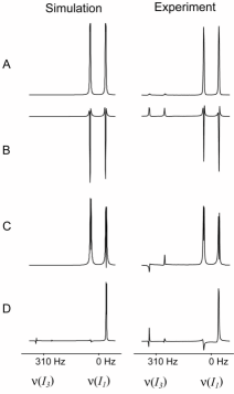
Figure 4: Simulated (left) and experimental (right) ¹H spectra of the amino moiety of ¹⁵N acetamide with $J_{12}=-87.3$ Hz, $J_{23}=-88.8$ Hz and $J_{13}=2.9$ Hz. Starting from thermal equilibrium, in all experiments the state $\rho_{A}=I_{1x}$ was prepared by saturating spins $I_{2}$ and $I_{3}$ and applying a $90^{\circ}_{y}$ pulse to spin $I_{1}$. (A) Spectrum corresponding to $\rho_{A}=I_{1x}$, (B) spectrum obtained after applying the propagator ${\cal U}_{13}=\exp\{-{\rm i}{\pi\over 2}\ 2I_{1z}I_{3z}\}$ to $\rho_{A}$, (C) resulting spectrum after applying the propagator $\sqrt{{\cal U}_{13}}=\exp\{-{\rm i}{\pi\over 4}\ 2I_{1z}I_{3z}\}$ to $\rho_{A}$, (D) spectrum after applying the Toffoli gate to $\rho_{A}$.

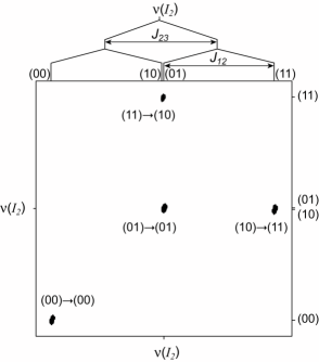
Figure 5: Experimental two-dimensional ¹⁵N spectrum of ¹⁵N acetamide representing the effect of the CNOT(1,3) gate. Using the relation CNOT(1,3)=$\exp\{-{\rm i}{\pi\over 2}(I_{1z}-I_{3z})\}\exp\{-{\rm i}{\pi\over 2}I_{3x}\}{\cal U}_{13}\exp\{-{\rm i}{\pi\over 2}I_{3y}\}$, the experimental pulse sequence was based on the implementation of the propagator ${\cal U}_{13}$ shown in Fig. 3 A.

In Fig. 3, schematic representations of the pulse sequences based on sub-Riemannian geodesics are shown for the efficient implementation of ${\cal U}_{13}$ and $\sqrt{{\cal U}_{13}}$ simulating coupling evolution by angles ${\pi\over 2}$ (Fig. 3 A) and ${\pi\over 4}$ (Fig. 3 B) between indirectly coupled qubits. As shown above, it is straight-forward to construct CNOT(1,3) from ${\cal U}_{13}$, which differ only by local rotations. Based on $\sqrt{{\cal U}_{13}}$, it is also possible to construct an efficient implementation of the Toffoli gate (Fig. 3 C). For simplicity, in Fig. 3 it is assumed that qubits $I_{1}$, $I_{2}$, and $I_{3}$ are on resonance in their respective rotating frames, coupling constants are positive ($J_{12}=J_{23}=J>0$ and $J_{13}=0$) and hard spin-selective pulses (of negligible duration) are available. More realistic pulse sequences which compensate off-resonance effects by refocusing pulses and practical pulse sequences are given in the supplementary material.

For an experimental demonstration of the proposed pulse sequence elements, we chose the amino moiety of ¹⁵N acetamide (NH₂COCH₃) dissolved in DMSO-d₆ [23]. NMR experiments were performed at a temperature of 295 K using a Bruker 500 MHz Avance spectrometer. Spins $I_{1}$ and $I_{3}$ are represented by the amino ¹H nuclear spins and spin $I_{2}$ corresponds to the ¹⁵N nuclear spin. The scalar couplings of interest are $J_{12}=-87.3$ Hz $\approx J_{23}=-88.8$ Hz and $J_{13}=2.9$ Hz. The actual pulse sequences implemented on the spectrometer and further experimental details are given in the supplementary material.

The propagators of the constructed pulse sequences were tested numerically and we also performed a large number of experimental tests. For example, Fig. 4 shows a series of simulated and experimental ¹H spectra of the amino moiety of ¹⁵N acetamide. In the simulations, the experimentally determined coupling constants and resonance offsets of the spins were taken into account. The various propagators were calculated for the actually implemented pulse sequences (given in the supplementary material) neglecting relaxation effects. In the simulated spectra, a line broadening of 3.2 Hz was applied in order to facilitate the comparison with the experimental spectra. Starting at thermal equilibrium, the state

$$\rho_{A}=I_{1x}$$

can be conveniently prepared by saturating spins $I_{2}$ and $I_{3}$ and applying a $90^{\circ}_{y}$ pulse to spin $I_{1}$. The resulting spectrum with an absorptive in-phase signal of spin $I_{1}$ is shown in Fig. 4 A.

Application of the propagator $U_{13}=\exp\{-{\rm i}{\pi\over 2}\ 2I_{1z}I_{3z}\}$ to $\rho_{A}$ results in the state

$$\rho_{B}=2I_{1y}I_{3z}.$$

The corresponding spectrum shows dispersive signal of spin $I_{1}$ in antiphase with respect to spin $I_{3}$, see Fig. 4 B.

The propagator $\sqrt{U_{13}}=\exp\{-{\rm i}{\pi\over 4}\ 2I_{1z}I_{3z}\}$ transforms the prepared state $\rho_{A}$ into

$$\rho_{C}={1\over\sqrt{2}}(I_{1x}+2I_{1y}I_{3z}),$$

resulting in a superposition of absorptive in-phase and dispersive antiphase signals of spin $I_{1}$, see Fig. 4 C.

The Toffoli gate applied to $\rho_{A}$ yields

$$\rho_{D}={1\over\sqrt{2}}(I_{1x}+2I_{1x}I_{2z}+2I_{1x}I_{3x}-4I_{1x}I_{2z}I_{3x}).$$

Only the first two terms in $\rho_{D}$ give rise to detectable signals. The corresponding spectrum is a superposition of an absorptive in-phase signal of spin $I_{1}$ and an absorptive antiphase signal of spin $I_{1}$ with respect to spin $I_{2}$, resulting in the spectrum shown in Fig. 4 D.

The effect of the $CNOT(1,3)$ gate can be conveniently demonstrated by using a two-dimensional experiment [24]. Fig. 6 shows the resulting two-dimensional spectrum of the ¹⁵N multiplet (corresponding to spin $I_{2}$) which reflects the expected transformations of the spin states of $I_{1}$ and $I_{3}$ under the $CNOT(1,3)$ operation.

5 Conclusion

In this manuscript, we have shown that problems of efficient synthesis of couplings between indirectly coupled qubits can be solved by reducing them to problems in geometry. We have constructed efficient ways of synthesizing quantum gates on a linear spin chain with Ising couplings including CNOT and Toffoli operations. We showed significant savings in time in implementing these quantum gates over state-of-the-art methods. We believe, the mathematical methods presented here will have applications to broad areas of quantum information technology. The quantum gate design metric $\frac{|dw|^{2}}{1-|w|^{2}}$ defined on a open unit disc in a complex plane could play an interesting role in the subject of quantum information.

The methods presented are expected to have applications to recent proposals of making nuclear spins acting as client qubits [16] share information efficiently via distributed hyperfine coupling to an electron spin $\frac{1}{2}$ acting as the bus-qubit. Efficient synthesis of couplings between indirectly coupled spins will also be very useful in multidimensional NMR applications to correlate the frequencies of spins $1$ and $3$ coupled indirectly through spin $2$ [17]. Recent numerical optimization studies [25, 26] indicate that the gap between conventional and time optimal methods for synthesis of typical quantum circuits, (for e.g. quantum Fourier transform) on practical architectures, increases rapidly with the number of qubits. This motivates further mathematical developments along the lines of the present work in searching for time optimal techniques of manipulating coupled spin systems. In practical quantum computing, this might prove to be very important as minimizing decoherence losses by efficient gate synthesis improves the fidelity of gates. Since fault tolerent quantum computing protocols require gates to have a fidelity above a certain threshold, optimal gate synthesis methods like presented here could prove critical in practical quantum computing. The problem of constrained optimization that arises in time optimal synthesis of unitary transformations in spin networks is also expected to instigate new ideas and method development in fields of optimal control and geometry.

6 Supplementary material

The ¹H and ¹⁵N transmitter frequencies were set on resonance for spins $I_{1}$ and $I_{2}$, respectively. The frequency difference between spins $I_{1}$ and $I_{3}$ was $\Delta\nu_{13}=310$ Hz. Selective rotations of the ¹⁵N nuclear spin $I_{2}$ were implemented using hard pulses. Spin-selective proton pulses were realized by combinations of hard pulses and delays in our experiments. For example, a selective $90^{\circ}$ rotation of spin $I_{3}$ with phase $y$, denoted $90^{\circ}_{y}(I_{3})$, is realized by the sequence element $90^{\circ}_{x}(I_{1},I_{3})-(\Delta_{1}/2)-180^{\circ}_{x}(I_{2})-(\Delta_{1}/2)-180^{\circ}_{x}(I_{2})\ 90^{\circ}_{-x}(I_{1},I_{3})$, where $\Delta_{1}=1/(4\Delta\nu_{13})$ and $90^{\circ}_{\pm x}(I_{1},I_{3})$ correspond to non-selective (hard) proton pulses, acting simultaneously on $I_{1}$ and $I_{3}$. Figures 6 A - 8 A show broadband versions of the ideal sequence shown in Fig. 3, which are robust with respect to frequency offsets of the spins. Positive coupling constants $J_{12}=J_{23}=J>0$ (with $J_{13}=0$) and hard spin-selective pulses are assumed. Figures 6 B - 8 B show the actual pulse sequences used in the experiments with the ¹⁵N acetamide model system. In the experimental pulse sequences, selective ¹H pulses were implemented using hard pulses and delays, where $\Delta_{1}=1/(4\Delta\nu_{13})$. Furthermore, the sequences were adjusted to take into account that in the experimental model system the couplings $J_{12}$ and $J_{23}$ are negative. Broadband implementations of weak irradiation periods [23] are enclosed in brackets and the number $m$ of repetitions was two in all experiments.

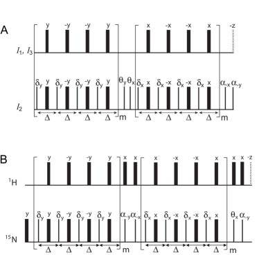
Figure 6: (A) Broadband version of the ideal $U_{13}$ sequence shown in Fig. 3 A, which is robust with respect to frequency offsets of the spins. Positive coupling constants $J_{12}=J_{23}=J>0$ (with $J_{13}=0$) and hard spin-selective pulses are assumed. The delay $\Delta$ is $\tau/(4m)$ and the flip angle $\delta$ is $2\pi\nu_{a}\tau/(4m)=0.5119/m$ (corresponding to $29.33^{\circ}/m$). (B) Experimentally implemented pulse sequence synthesizing ${\cal U}_{13}$ for the spin system of ¹⁵N acetamide with $J(^{1}$H,¹⁵N)$\ \approx-88$ Hz, $m=2$, flip angles $\alpha=148.6^{\circ}$, $\theta=31.4^{\circ}$ and $\delta=14.66^{\circ}$ and delay $\Delta=890.2$ $\mu$s. Narrow and wide bars correspond to $90^{\circ}$ and $180^{\circ}$ pulses, respectively, if no other flip angle is indicated, $z$-rotations are represented by dashed bars.

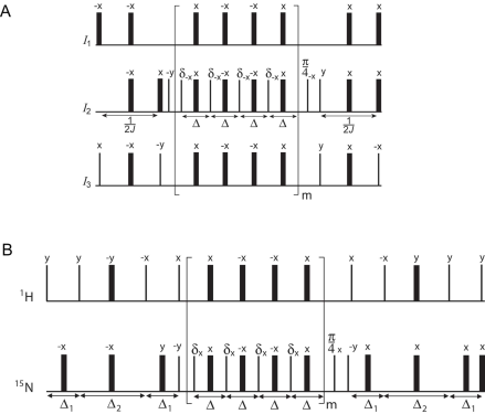
Figure 7: (A) Broadband version of the ideal $\sqrt{{\cal U}_{13}}$ sequence shown in Fig. 3 B, which is robust with respect to frequency offsets of the spins. Positive coupling constants $J_{12}=J_{23}=J>0$ (with $J_{13}=0$) and hard spin-selective pulses are assumed. The delay $\Delta$ is $\sqrt{7}/(16mJ)=0.1654/(mJ)$ and the flip angle $\delta$ is $3\pi/(8m)$ (corresponding to $67.5^{\circ}/m$). (B) Experimentally implemented pulse sequence synthesizing $\sqrt{{\cal U}_{13}}$ for the spin system of ¹⁵N acetamide with $J(^{1}$H,¹⁵N)$\ \approx-88$ Hz, $\exp\{-{\rm i}\ (\pi/2)\ I_{1z}I_{3z}\}$ for $J(^{1}$H,¹⁵N)$\ \approx-88$ Hz with $m=2$, $\delta=33.75^{\circ}$, $\Delta=\sqrt{7}/(16m|J(^{1}$H,¹⁵N)$|)=939.5$ $\mu$s, $\Delta_{1}=1/(4\Delta\nu_{13})=806.5$ $\mu$s and $\Delta_{2}=1/(2|J(^{1}$H,¹⁵N)$|)=5.68$ ms.

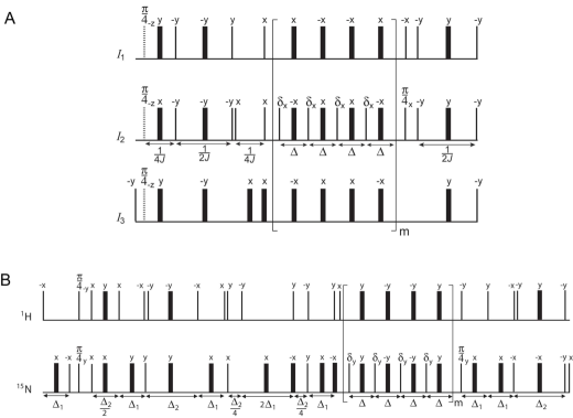
Figure 8: Broadband version of the ideal Toffoli sequence shown in Fig. 3 B, which is robust with respect to frequency offsets of the spins. Positive coupling constants $J_{12}=J_{23}=J>0$ (with $J_{13}=0$) and hard spin-selective pulses are assumed. (B) Experimentally implemented pulse sequence synthesizing a Toffoli gate for the spin system of ¹⁵N acetamide. Delays $\Delta$, $\Delta_{1}$, $\Delta_{2}$ and the small flip angle $\delta$ are defined in Fig. 7.

References

- [1] P.W. Shor, Proceedings of the 35th Annual Symposium on Fundamentals of Computer Science, (IEEE Press, Los Alamitos, CA, 1994).
- [2] M.A. Nielsen and I.L. Chuang, Quantum Information and Computation, (Cambridge Unniversity Press, 2000).
- [3] M. A. Nielsen, M. R. Dowling, M . Gu, A. C. Doherty, Science 311, 1133-1135 (2006).
- [4] N. Khaneja, R. W. Brockett, S. J. Glaser, Phys. Rev. A 63, 03208 (2001).
- [5] T. O. Reiss, N. Khaneja, S. J. Glaser, J. Magn. Reson. 154, 192-195 (2002).
- [6] H. Yuan and N. Khaneja, Phys. Rev. A 72 040301(R) (2005).
- [7] G. Vidal, K. Hammerer and J. I. Cirac, Phys. Rev. Lett. 88, 237902 (2002).
- [8] N. Khaneja, S. J. Glaser, R. W. Brockett, Phys. Rev. A 65, 032301 (2002).
- [9] N. Khaneja, F. Kramer, S. J. Glaser, J. Magn. Reson. 173, 116-124 (2005).
- [10] N. Khaneja, S. J. Glaser, Physical Review A 66, 060301(R) (2002).
- [11] R.W. Brockett, in New Directions in Applied Mathematics, P. Hilton and G. Young (eds.), Springer-Verlag, New York, 1981.
- [12] J. Baillieul, Ph.D. thesis, Harvard Univ., Applied Math (1975).
- [13] R. Montgomery, “A Tour of Subriemannian Geometries, their Geodesics and Applications”, American Mathematical Society, 2002.
- [14] B.E. Kane, Nature 393, 133-137 (1998).
- [15] F. Yamaguchi, Y. Yamamoto, Appl. Phys. A 68, 1-8 (1999).
- [16] M. Mehring, J. Mende and W. Scherer, Phys. Rev. Lett. 90, 153001 (2003).
- [17] R. R. Ernst, G. Bodenhausen, A. Wokaun, Principles of Nuclear Magnetic Resonance in One and Two Dimensions, (Clarendon Press, Oxford, 1987).
- [18] T. Toffoli, Math. Systems Theory 14, 13-23 (1981).
- [19] T. Sleator and H. Weinfurter, Phys. Rev. Lett. 74, 4087-4090 (1995).
- [20] D. P. DiVincenzo, Proc. Royal Soc. London A 1969, 261-276 (1998).
- [21] James. W. Anderson, Hyperbolic Geometry, (Springer Verlag, London, 2001).
- [22] D. Collins, K. W. Kim, W. C. Holton, H. Sierzputowska-Gracz, E. O. Stejskal, Phys. Rev. A 62, 022304 (2000).
- [23] T. O. Reiss, N. Khaneja, S. J. Glaser, J. Magn. Reson. 165, 95-101 (2003).
- [24] Z. L. Mádi. R. Brüschweiler, R. R. Ernst, J. Chem. Phys. 109, 10603-10611 (1998).
- [25] N. Khaneja, T. Reiss, C. Kehlet, T. Schulte-Herbrüggen, S. J. Glaser, J. Magn. Reson. 172, 296-305 (2005).
- [26] T. Schulte-Herbrüggen, A.K. Spörl, N. Khaneja, S.J. Glaser, Phys. Rev. A 72, 042331 (2005).