Efficiency limits for linear optical processing of single photons and single-rail qubits

Abstract

We analyze the problem of increasing the efficiency of single-photon sources or single-rail photonic qubits via linear optical processing and destructive conditional measurements. In contrast to previous work we allow for the use of coherent states and do not limit to photon-counting measurements. We conjecture that it is not possible to increase the efficiency, prove this conjecture for several important special cases, and provide extensive numerical results for the general case.

I Introduction

The single-photon state of light is one of the primary resources in quantum information technology. It is indispensable in linear optical quantum computing LOQC1 ; LOQC2 and essential for many protocols of quantum communication. However, existing single-photon sources photonsources are far from perfect. Whereas most ensure that the optical output contains negligible multi-photon terms, there is always a significant probability that the desired single photon itself is not emitted into the desired optical mode or is lost at a later stage. As a result, the optical state generated by typical single-photon sources can be described as an incoherent mixture of the single-photon and vacuum states, namely

$$\hat{\rho}=p|{1}\rangle\langle{1}|+(1-p)|{0}\rangle\langle{0}|.$$ (1)

We call this state an inefficient single photon with efficiency $p$. The efficiency of most existing photon sources is much lower than that desirable in many quantum-information processing protocols.

Theoretically, the efficiency of state (1) can be improved by nonlinear optical means, such as quantum nondemolition measurements in the photon-number basis QNDNL1 ; QNDNL2 . However, this approach is not practical because materials that combine the required nonlinearity with low optical losses are not available at present. Therefore, it would be desirable to improve the efficiency by means of linear optical processing (i.e. interferometry) and destructive conditional measurements.

The possibility of such an improvement was investigated by Berry and co-workers berry1 ; berry2 , who considered a general interferometric circuit with $N$ inefficient single photons as inputs. All output modes except one were subject to photon number measurements, and the quantum state of the remaining mode, conditioned on a particular result of this measurement, was analyzed. It was found that the single-photon component could be increased, but at the expense of introducing multiphoton components. It was also shown that no efficiency improvement can be achieved if the total number of photons detected equals $0$, $1$, or $N-1$.

A closely related problem is that of the processing of single-rail photonic qubits. A single-rail qubit (SRQ) is a qubit with basis comprising the vacuum state and single-photon state of one optical mode. An inefficient single photon is a special case of a SRQ. Berry, Lvovsky, and Sanders berry generalized the notion of photon efficiency to SRQs, and showed that a single-rail qubit can be converted, by means of linear optical processing and conditional measurements, into a qubit of a different value (including the inefficient single photon) with arbitrarily low loss of generalized efficiency. Therefore, the problem of increasing the efficiency of single-photon sources is largely equivalent to the problem of increasing the efficiency of SRQs.

There are a number of alternative approaches to converting a SRQ to an inefficient single photon. A range of examples are presented in Appendix Appendix A: Example schemes. A notable feature of these schemes is that they use resources such as coherent states and general projective measurements for the processing; these resources were not considered in earlier work on processing single-photon sources berry1 ; berry2 . Here we examine general processing including these resources, and show that all the results found for more restricted processing also hold when we allow coherent states and general measurements.

Another feature of the schemes presented in the Appendix is that they involve processing of up to two sources. In previous work berry it was only shown that the SRQ efficiency could not be increased for processing of one SRQ. Here we show that the same result holds for processing of up to two SRQs. In general, we conjecture that it is not possible to improve the efficiency of SRQs or single photons by means of linear optics and destructive measurements (without introducing a multiphoton component). Although we do not prove this conjecture, we do show its validity for a variety of cases, and significantly restrict the class of apparatuses in which efficiency improvement might be achieved. We furthermore provide extensive numerical results that support this conjecture in the general case.

We begin by defining the general problem, and give a list of simplifications that can be made (Sec. II). Then we present the general conjecture that it is impossible to increase the efficiency, even allowing for the use of coherent states and general measurements, in Sec. III. In Sec. IV we prove the conjecture for some important special cases, which are analogous to those studied in the case where measurements are limited to photon counting berry1 ; berry2 . Numerical results in support of the conjecture are presented in Sec. V. In Sec. VI we utilize the results of previous work berry to generalize the results to single-rail optical qubits. Conclusions are given in Sec. VII.

II General processing and simplifications

II.1 The formulation of the problem

Fig. 1 displays a general scheme for processing modes by means of linear optics and destructive measurements. In the general case the input states $\hat{\rho}_{1},\ldots,\hat{\rho}_{N_{1}}$ are single-rail qubits. We address this case in Sec. VI; here we restrict these inputs to be inefficient single-photon sources. We consider a more general form of processing than that in previous work berry1 ; berry2 , and allow coherent state inputs and general measurements on the outputs. We have $N_{1}$ single-photon sources with efficiencies $p_{i}$, and $N-N_{1}$ coherent states $|{\alpha_{N_{1}+1}}\rangle,\ldots,|{\alpha_{N}}\rangle$ (the vacuum state is also permitted by taking $\alpha_{j}=0$). All inputs are processed by a linear optical interferometer, and all output channels except channel 1 are subjected to a general destructive measurement. Conditioned on a particular result of this measurement, we analyze the quantum state $\hat{\rho}_{\rm out}$ of the remaining mode.

Figure 1: General processing of multiple SRQs or single-photon sources.

We restrict our treatment to schemes in which the output state has no multiphoton ($n\geq 2$) components. For additional generality, in the case where coherent states are used, we allow the possibility that the multiphoton components are small but nonzero, and take a limit where they approach zero. This is to take account of schemes such as Scheme 2 in the Appendix, which requires such a limit.

The goal is to either find a scheme in which the output state has an efficiency that is higher than the highest of the input single-photon efficiencies ($p_{\rm max}$) under this restriction on the multiphoton components, or to prove that such a scheme does not exist. In this section, we show that if a scheme able to enhance the photon efficiency does exist, it can be simplified in a number of ways without losing this property. In this way, we restrict the class of schemes in which the desired effect should be sought. It is important that these simplifications are performed in the order listed because, in some steps, we assume that previous simplifications have already been made while subsequent ones have not.

We exclude feedback or feedforward because their effect can be reproduced in a conditional measurement setting, which is accommodated in our formalism. Because we permit vacuum inputs and generalized measurements, we can also assume, without loss of generality, that the interferometer is lossless and has an equal number of input and output channels.

For this general processing the output state can be a single-rail qubit (with coherence between the vacuum and single-photon components), rather than just an inefficient single photon. Here we simply characterize the efficiency of the output by the single-photon probability, rather than the SRQ generalized efficiency berry , which is treated later in Sec. VI.

Next we define our notation. The input and output states of the $N$ interferometer channels are called $\hat{\rho}_{\rm in}$ and $\hat{\rho}_{\rm trans}$, respectively. The interferometer itself is characterized by a unitary operator $\hat{U}$ (so that $\hat{\rho}_{\rm trans}=\hat{U}\hat{\rho}_{\rm in}\hat{U}^{\dagger}$). In the Heisenberg representation, we associate the interferometer with unitary matrix ${\bf\Lambda}$ (throughout the paper, we use boldface to indicate vectors and matrices) such that the amplitude operators of the input and output modes are transformed according to

$$\hat{a}_{{\rm in},i}^{\dagger}\mapsto\sum_{k}\Lambda_{ki}\hat{a}_{{\rm out},k}^{\dagger}.$$ (2)

We describe the measurement on the interferometer output modes $2,\ldots,N$ by some positive operator-valued measure, and $\hat{\rho}_{\rm out}$ is conditioned on its element $\hat{M}$, so that

$$\hat{\rho}_{\rm out}=K{\rm Tr}_{2\cdots N}(\hat{M}\hat{\rho}_{\rm trans}),$$ (3)

where $K$ is the normalization constant that accounts for a loss of normalization in a partial measurement of a multipartite state. The probability that the output state contains $n_{1}$ photons is denoted by $c_{n_{1}}$ (i.e. $\langle{n_{1}}|\hat{\rho}_{\rm out}|{n_{1}}\rangle=c_{n_{1}}$). We thus wish to achieve the condition $c_{1}>p_{\rm max}$ and, at the same time, $\sum_{n_{1}>2}c_{n_{1}}\to 0$.

II.2 Coherent state inputs

Here we show that, without loss of generality, all the coherent state inputs may be chosen to be vacuum states. The state with the coherent state inputs replaced with vacuum is denoted $\hat{\rho}_{0}$. The original input state $\hat{\rho}_{\rm in}$ is obtained from $\hat{\rho}_{0}$ by applying displacement operators

$$\hat{D}_{i}(\alpha_{i})=\exp(\alpha_{i}\hat{a}_{i}^{\dagger}-\alpha_{i}^{*}\hat{a}_{i})$$ (4)

to each input $i$ ($N_{1}<i\leq N$). The input state may then be expressed as

$$\hat{\rho}_{\rm in}=\left[\prod_{i=N_{1}+1}^{N}\hat{D}_{i}(\alpha_{i})\right]\hat{\rho}_{0}\left[\prod_{i=N_{1}+1}^{N}\hat{D}_{i}(-\alpha_{i})\right].$$ (5)

The interferometer transforms each $\hat{a}_{i}$ according to Eq. (2) and produces the state

$$\hat{\rho}_{\rm trans}=\left[\prod_{k=1}^{N}\hat{D}_{k}(\alpha^{\prime}_{k})\right]\hat{U}\hat{\rho}_{0}\hat{U}^{\dagger}\left[\prod_{k=1}^{N}\hat{D}_{k}(-\alpha^{\prime}_{k})\right].$$ (6)

where, in accordance with Eq. (4), $\alpha^{\prime}_{k}=\sum_{i=N_{1}+1}^{N}\alpha_{i}\Lambda_{ki}$.

Projection onto state $|{\chi}\rangle$ for modes 2 to $N$ yields the output state that can be written as

$$\hat{\rho}_{\rm out}\propto\hat{D}_{1}(\alpha^{\prime}_{1})\left[{\rm Tr}_{2\ldots N}(\hat{M}^{\prime}\hat{U}\hat{\rho}_{0}\hat{U}^{\dagger})\right]\hat{D}_{1}(-\alpha^{\prime}_{1}),$$ (7)

where

$$\hat{M}^{\prime}=\left[\prod_{k>1}\hat{D}_{k}(-\alpha^{\prime}_{k})\right]\hat{M}\left[\prod_{k>1}\hat{D}_{k}(\alpha^{\prime}_{k})\right].$$ (8)

A displacement operator acting on a state with a finite photon number will necessarily yield nonzero coefficients for arbitrarily large photon number. If we require that the multiphoton components in the output are negligible, then we must take the limit $\alpha^{\prime}_{1}\to 0$. Our original scheme with the input state $\hat{\rho}_{\rm in}$ and conditioning on measurement result corresponding to the application of $\hat{M}$ is then equivalent to a scheme with the same interferometer, all coherent states in the input replaced by vacuum, and measurement corresponding to $\hat{M}^{\prime}$.

The motivation for including the possibility of the multiphoton components approaching zero in a limit in the above discussion is that there are cases where this is useful when coherent states are permitted (see the Appendix for an example). There does not appear to be any reason for allowing this possibility in the absence of coherent state inputs, so in the remainder of this paper we restrict the multiphoton components to be strictly zero.

Note that the above derivation does not rely on the particular form of the states on which the displacements act. In particular, we could have included displacements on the single-photon sources; the above derivation shows that such displacements would not increase the power of the processing. One could therefore define an efficiency for displaced single-photon sources (or displaced SRQs) that is equal to the efficiency of the state without the displacement.

II.3 Unequal efficiencies and vacuum inputs

We now make the simplification that we need not use inputs with different efficiencies. We obtain two slightly different results.

1. The maximum output efficiency may be obtained without modifying the interferometer and taking all inputs to either have efficiency $p_{\rm max}$ or be the vacuum.

2. For any interferometer which achieves a certain output efficiency, we may achieve an efficiency at least as large with a modified interferometer and all inputs with efficiency $p_{\rm max}$.

Note the difference in these results: in the first we use the same interferometer, and in the second we allow a modified interferometer.

To prove the first result, we note that the input state for $p_{i}\leq p_{\rm max}$ is just a convex combination of states with all efficiencies either $p_{\rm max}$ or 0 (vacuum). Thus the output state is again a convex combination, though with possibly different weightings. The single-photon probability must be maximized for one of the states in this convex combination, and therefore is maximized for all efficiencies either $p_{\rm max}$ or 0. This result holds regardless of whether we require the multiphoton components to be zero. Clearly if the multiphoton components are zero for the output state with $p_{i}\leq p_{\rm max}$, they are zero for all states in the convex combination.

For the second result, we note that we can achieve a vacuum state simply by combining two single-photon sources at a beam splitter and conditioning on detection of two photons in one of the beam splitter outputs. (Note that the beam splitter must be chosen such that the probability for detection of two photons is nonzero.) We may use the first result to show that all inputs can have efficiency either $p_{\rm max}$ or 0, then replace all the vacuum inputs with two sources with efficiency $p_{\rm max}$. Thus we see that any efficiency we can achieve with vacuum inputs can also be achieved with all inputs identical, although with a modified interferometer.

We now show that, in order to obtain the second result, it is not necessary to expand the interferometer by more than one mode. First let us consider a scheme with all inputs with efficiency either $p_{\rm max}$ or 0, and sort all the vacuum inputs to the right, as in Fig. 2(a). We may then simplify the scheme to a line of beam splitters followed by a $U(N-1)$ interferometer on modes 2 to $N$, then measurement on modes 2 to $N$. The $U(N-1)$ interferometer and measurement may be combined into a single measurement, as in Fig. 2(b).

Figure 2: A method of simplifying a scheme with multiple vacuum inputs.

Now the line of beam splitters acting on the vacuum inputs simply give vacuum outputs. Only one of these vacuum outputs is combined with non-vacuum states at further beam splitters; the remainder remain in the vacuum state. Conditional measurement on these modes does not affect the output state. These output modes, and the corresponding input modes can be thus removed from the interferometer, which simplifies the scheme to one which uses only one vacuum input.

We can replace that one vacuum input with two inputs with efficiency $p_{\rm max}$, as discussed above. Overall the number of modes needed is just $N_{1}+2$. If $N_{1}$ was equal to $N$, then there were no vacuum inputs, so we do not expand the interferometer. Otherwise the total number of modes needed is no more than $N+1$. Thus we can simplify the scheme to one with all identical inputs, and need not increase the number of modes by any more than $1$.

II.4 General measurements

The maximum output efficiency may be obtained using a projective measurement, rather than a more general measurement operator. The measurement on modes 2 to $N$ may be decomposed into projection operators as $\hat{M}=\sum_{i}q_{i}|{\chi_{i}}\rangle\langle{\chi_{i}}|$, so the output state will then be

$$\hat{\rho}_{\rm out}\propto\sum_{i}q_{i}\langle{\chi_{i}}|\hat{\rho}_{\rm trans}|{\chi_{i}}\rangle.$$ (9)

Thus

$$\hat{\rho}_{\rm out}=\sum_{i}q^{\prime}_{i}\hat{\rho}_{{\rm out},i}$$ (10)

for some probabilities $q^{\prime}_{i}$ with $\hat{\rho}_{{\rm out},i}\propto\langle{\chi_{i}}|\hat{\rho}_{\rm trans}|{\chi_{i}}\rangle$. Hence the single-photon probability for $\hat{\rho}_{\rm out}$ is a convex sum over that for the $\hat{\rho}_{{\rm out},i}$, and the maximum must be achieved for one of the $\hat{\rho}_{{\rm out},i}$. Therefore we see that the optimal result may be obtained via projective measurements.

II.5 Projections over different total photon numbers

Next we show that the state $|{\chi}\rangle$ associated with the projective measurement on modes 2 to $N$ does not need to be a superposition over different total numbers of photons. This result holds true when there is no coherent superposition over different total photon numbers in the input state. We may assume this to be the case because we have shown that coherent state inputs may be omitted. Because the interferometer does not change the total number of photons, its output state can be written as

$$\hat{\rho}_{\rm trans}=\sum_{L}p_{L}\hat{\rho}_{{\rm trans},L},$$ (11)

where $\hat{\rho}_{{\rm trans},L}$ denotes a state with a total of $L$ photons in the output modes. Similarly, we can write the projection state as a superposition

$$|{\chi}\rangle=\sum_{D}x_{D}|{\chi_{D}}\rangle,$$ (12)

where $|{\chi_{D}}\rangle$ is a normalized state containing terms with a total of $D$ photons. The probability that mode 1 contains $n_{1}$ photons is thus

$$c_{n_{1}}= K\langle{n_{1}}|\hat{\rho}_{\rm out}|{n_{1}}\rangle=K\langle{n_{1}}|\langle{\chi}|\hat{\rho}_{\rm trans}|{\chi}\rangle|{n_{1}}\rangle$$

$$= K\sum_{L}p_{L}\sum_{D,D^{\prime}}x_{D}^{*}x_{D^{\prime}}\langle{n_{1}}|\langle{\chi_{D}}|\hat{\rho}_{{\rm trans},L}|{\chi_{D^{\prime}}}\rangle|{n_{1}}\rangle.$$ (13)

We now notice that the above matrix element is nonzero only if $D=D^{\prime}=L-n_{1}$. We can therefore write, specifically for $n_{1}=1$,

$$c_{1}=K\sum_{L}p_{L}|x_{L-1}|^{2}\langle{1}|\langle{\chi_{L-1}}|\hat{\rho}_{{\rm trans},L}|{\chi_{L-1}}\rangle|{1}\rangle.$$ (14)

This is a convex sum and must reach a maximum for $x_{L-1}$ equal to 1 for one specific value of $L=L_{0}$ and 0 for others. If the projection state $|{\chi}\rangle$ is replaced by $|{\chi_{L_{0}-1}}\rangle$ (which does not contain superpositions of different total number of photons), the value of $c_{1}$ will increase or remain the same, which completes the proof.

III General conjecture

III.1 The conjecture

In this section, we conjecture that it is not possible to improve the single photon efficiency provided the multiphoton component in $\hat{\rho}_{\rm out}$ is zero. This conjecture may be expressed in the following way:

$$\sum_{n_{1}=2}^{N}c_{n_{1}}=0\implies c_{1}\leq p_{\rm max},$$ (15)

where $p_{\rm max}$ is the highest of the input source efficiencies.

This form is somewhat inconvenient to use in numerical testing, as it has a large number of independent efficiencies $p_{i}$. Therefore, in the subsequent treatment, we invoke the simplification of Sec. II.3 and assume that all input channels are in the state (1) with $p_{i}=p_{\rm max}$. In order to formally express our conjecture, we write the circuit input as a probabilistic mixture of pure states defined by vector ${\bm{s}}=(s_{1},\ldots,s_{N})$, where $s_{i}=0$ or 1 determines whether the photon is present in the $i^{\text{th}}$ input channel:

$$\hat{\rho}_{\rm in}=\sum_{\bm{s}}P_{\bm{s}}\left[\prod_{i}(\hat{a}_{i}^{\dagger})^{s_{i}}|{0}\rangle\langle{0}|\prod_{i}\left(\hat{a}_{i}\right)^{s_{i}}\right],$$ (16)

where

$$P_{\bm{s}}=p_{\rm max}^{\Sigma_{\bm{s}}}(1-p_{\rm max})^{N-\Sigma_{\bm{s}}}$$ (17)

is the probability of occurrence for a particular vector ${\bm{s}}$, $\Sigma_{\bm{s}}$ being the number of nonzero elements in ${\bm{s}}$. The interferometer maps the operator of every mode according to Eq. (2), thus producing the state

$$\hat{\rho}_{\rm trans}=\sum_{\bm{s}}P_{\bm{s}}\prod_{i}\left(\sum_{k}\Lambda_{ki}\hat{a}_{k}^{\dagger}\right)^{\!\!s_{i}}\!\!|{0}\rangle\langle{0}|\prod_{i}\left(\sum_{k}\Lambda_{ki}^{*}\hat{a}_{k}\right)^{\!\!s_{i}}\!.$$ (18)

If modes 2 to $N$ are projected onto state $|{\chi}\rangle$, the probability that mode 1 contains $n_{1}$ photons is

$$c_{1}=K\langle{n_{1}}|\langle{\chi}|\hat{\rho}_{\rm trans}|{\chi}\rangle|{n_{1}}\rangle=K\sum_{\bm{s}}P_{\bm{s}}|T_{{\bm{s}},\chi}^{(n_{1})}|^{2},$$ (19)

where we have introduced the quantity

$$T_{{\bf s},\chi}^{(n_{1})}=\langle{n_{1}}|\langle{\chi}|\prod_{i}\left(\sum_{k}\Lambda_{ki}\hat{a}_{k}^{\dagger}\right)^{s_{i}}|{0}\rangle,$$ (20)

which yields the amplitude of state $|{n_{1}}\rangle|{\chi}\rangle$ emerging in the interferometer output provided that the input state is determined by vector ${\bm{s}}$.

This amplitude has the important property

$$T_{\bm{s},\chi}^{(n_{1}+1)}=\frac{1}{\sqrt{n_{1}+1}}\sum_{i;s_{i}=1}\Lambda_{1i}T_{\bm{s}^{i},\chi}^{(n_{1})}$$ (21)

with ${\bf s}^{i}$ a vector identical to ${\bf s}$ except the $i^{\text{th}}$ position at which the value $1$ is replaced by $0$. Eq. (21) is proven in the next subsection. Eq. (21) implies that if $T_{\bm{s},\chi}^{(2)}=0$ for all $\bm{s}$, then $T_{\bm{s},\chi}^{(n_{1})}=0$ for all $\bm{s}$ and $n_{1}>2$. It then follows that if $c_{n_{1}}=0$ holds for $n_{1}=2$, it must also hold for all $n_{1}>2$.

The inequality $\langle{1}|\hat{\rho}_{\rm out}|{1}\rangle\leq p_{\rm max}$ in Eq. (15) is equivalent to

$$\sum_{\bm{s};\Sigma_{\bm{s}}=D+1}P_{\bm{s}}|T_{\bm{s},\chi}^{(1)}|^{2}\leq\frac{p_{\rm max}}{1-p_{\rm max}}\sum_{\bm{s};\Sigma_{\bm{s}}=D}P_{\bm{s}}|T_{\bm{s},\chi}^{(0)}|^{2},$$ (22)

where we have assumed, according to Sec. II.5, that the projection state $|{\chi}\rangle$ has a certain total number of photons $D$. Substituting the expression (17) for $P_{\bf s}$ into Eq. (22), we cancel all probability-related factors and rewrite our conjecture in the form

$$\sum_{\bm{s}}|T_{\bm{s},\chi}^{(2)}|^{2}=0\implies\sum_{\bm{s}}|T_{\bm{s},\chi}^{(1)}|^{2}\leq\sum_{\bm{s}}|T_{\bm{s},\chi}^{(0)}|^{2}.$$ (23)

This form is more useful than that given in the beginning of this section, because it does not depend on the probabilities.

III.2 Mathematical formulation

In this subsection, we develop a formalism that allows us to provide a formulation of the conjecture in a pure mathematical form that does not involve quantum amplitudes. We begin by decomposing the measurement state $|{\chi}\rangle$ into tensor products of Fock states

$$|{\chi}\rangle=\sum_{\bar{\bm{n}}}\chi_{\bar{\bm{n}}}|{\bar{\bm{n}}}\rangle,$$ (24)

where vector $\bar{\bm{n}}=(n_{2},\ldots,n_{N})$ determines the number of photons in modes 2 to $N$ of the interferometer output. We can then rewrite Eq. (20) as

$$T_{\bm{s},\chi}^{(n_{1})}=\sum_{\bar{\bm{n}}}\chi_{\bar{\bm{n}}}^{*}(\bm{n}!)^{-1/2}S_{\bm{s},\bm{n}},$$ (25)

where $\bm{n}=(n_{1},\ldots,n_{N})$ is the vector $\bar{\bm{n}}$ with the addition of the first mode, $\bm{n}!=\prod_{j=1}^{N}n_{j}!$ and

$$S_{\bm{s},\bm{n}}=(\bm{n}!)^{1/2}T_{\bm{s},\bar{\bm{n}}}^{(n_{1})}=(\bm{n}!)^{1/2}\langle{\bm{n}}|\prod_{i}\left(\sum_{k}\Lambda_{ki}\hat{a}_{k}^{\dagger}\right)^{s_{i}}|{0}\rangle.$$ (26)

A direct calculation shows that $S_{\bm{s},\bm{n}}=\text{per}(\bm{\Lambda}[\bm{n},\bm{s}])$, where ‘per’ is the permanent of a matrix, provided $\bm{s}$ and $\bm{n}$ correspond to the same total numbers of photons ($\sum_{i}s_{i}=\sum_{i}n_{i}$) and zero otherwise. $\bm{\Lambda}[\bm{n},\bm{s}]$ is a matrix obtained from $\bm{\Lambda}$ by repeating the $i$’th column of $\bm{\Lambda}$ $s_{i}$ times, and the $j$’th row $n_{j}$ times.

Similarly to the determinant, the permanent of a matrix can be expanded by minors, but with all the signs taken as positive mathworld . Therefore, if we define $\Gamma_{\bm{s},\bar{\bm{n}}}^{(n_{1})}=S_{\bm{s},\bm{n}}^{*}$, we can write

$$\Gamma_{\bm{s},\bar{\bm{n}}}^{(n_{1}+1)}=\sum_{i;s_{i}=1}\Lambda_{1i}\Gamma_{\bm{s},\bar{\bm{n}}}^{(n_{1})},$$ (27)

from which one immediately obtains Eq. (21).

With the introduced notation, we are now ready to present another form of our conjecture. By taking $\bm{\chi}$ to indicate the vector of values $\chi_{\bar{\bm{n}}}(\bar{\bm{n}}!)^{-1/2}$, we can rewrite Eq. (23) as follows

$$\bm{\chi}^{\dagger}{\bm{\Gamma}^{(2)}}^{\dagger}\bm{\Gamma}^{(2)}\bm{\chi}=0\implies\bm{\chi}^{\dagger}{\bm{\Gamma}^{(1)}}^{\dagger}\bm{\Gamma}^{(1)}\bm{\chi}\leq\bm{\chi}^{\dagger}{\bm{\Gamma}^{(0)}}^{\dagger}\bm{\Gamma}^{(0)}\bm{\chi},$$ (28)

for all vectors $\bm{\chi}$, where the product indicates summation over indices $\bm{s}$ and $\bar{\bm{n}}$. The conjecture is therefore that

$${\bm{\Gamma}^{(1)}}^{\dagger}\bm{\Gamma}^{(1)}\leq{\bm{\Gamma}^{(0)}}^{\dagger}\bm{\Gamma}^{(0)}$$ (29)

on the null space of $\bm{\Gamma}^{(2)}$.

We have not yet been able to find a general proof of this conjecture. In the following two sections, we give an analytical proof for some special cases (which may be used as a basis for a future general proof by induction) and report the results of numerical tests that support the conjecture.

IV Special cases

The conjecture (15) can be proven for certain special cases defined by the total number $D$ of photons detected in the measurement on modes $2$ to $N$. In particular, the case $D=N_{1}$ is trivial as it implies $c_{0}=1$. The case $D=0$ involves projection onto the state $|{\chi_{0}}\rangle=|{0,\ldots,0}\rangle$ and has been studied previously berry1 ; berry2 . Below we prove the conjecture for $D$ equal to $1$ and $N_{1}-1$. We then use these results to prove no-go theorems for $N\leq 3$ or $N_{1}\leq 2$. In this section we do not assume that the inputs are all identical (that $p_{i}=p_{\rm max}$ and $N_{1}=N$), except in the proof for $D=1$.

One might think that one needs to require $D\geq N_{1}-1$ in order to eliminate multiphoton components from the output. This is, however, not the case, the simplest counterexample being a $(N=2)$-mode interferometer with $\Lambda_{11}=\Lambda_{22}=1$, $\Lambda_{12}=\Lambda_{21}=0$ (i.e. direct connection of the input and output modes). Detection of vacuum in mode 2 ($D=0$) does not imply that mode 1 has multiphoton terms. Therefore, the proof for $D=N_{1}-1$ is not sufficient to prove the conjecture.

IV.1 $D=1$

Because $|{\chi}\rangle$ contains only one photon, we can write it as a superposition $|{\chi}\rangle=\sum_{i=2}^{N}\phi_{i}\hat{a}_{i}^{\dagger}|{0}\rangle$. If we introduce a unitary transformation $\{\hat{a}_{i}\}\mapsto\{\hat{b}_{i}\}$ on modes 2 to $N$ such that $\hat{b}^{\dagger}_{2}=\sum_{i=2}^{N}\phi_{i}\hat{a}_{i}^{\dagger}$, we can write

$$|{\chi}\rangle=\hat{b}^{\dagger}_{2}|{0}\rangle,$$ (30)

so the state $|{\chi}\rangle$ corresponds to a single photon in the optical mode defined by operator $\hat{b}_{2}$, and vacuum in the remaining modes ($\hat{b}_{3},\ldots,\hat{b}_{N}$). Because there exists an interferometer associated with any unitary transformation of optical modes Zeilingerunitary , a projection measurement onto state $|{\chi}\rangle$ can be achieved by processing the modes 2 to $N$ with an additional interferometer and counting photons in each output mode (Fig. 3).

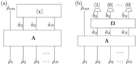
Figure 3: Projection onto a multimode state $|{\chi}\rangle$ with a total number of photons equal to 1 (a) can be replaced by processing with an additional interferometer (${\bf\Omega}$) and a photon counting measurement in each output (b).

Considering the two interferometers of Fig. 3(b) as a single interferometer, we find that the same output may be achieved with a modified interferometer and photon counting. It is known that, with photon counting measurements, $D=1$, $p_{i}=p_{\rm max}~{}\forall p_{i}$ and $N_{1}=N$, it is not possible to obtain increased efficiency berry1 ; berry2 . Thus we have found that this result also holds for general projection measurements that satisfy these conditions.

IV.2 $D=N_{1}-1$

We begin by rewriting Eq. (19) for the vacuum probability:

$$c_{0}=K\sum_{\bm{s};\Sigma_{\bm{s}}=D}P_{\bm{s}}|T_{\bm{s},\chi}^{(0)}|^{2}.$$ (31)

Following earlier reasoning concerning increasing the efficiency of single photon sources by interferometry and postselection based on photon counting berry1 ; berry2 , we notice that any input vector ${\bm{s}}$ with $D$ nonzero elements can be obtained from $N_{1}-D$ vectors with $D+1$ nonzero elements by setting one of their elements to zero. We write

$$c_{0}=\frac{K}{N_{1}-D}\sum_{\begin{subarray}{c}\bm{s};P_{\bm{s}}\neq 0\\ \Sigma_{\bm{s}}=D+1\end{subarray}}\sum_{k;s_{k}=1}P_{\bm{s^{k}}}|T_{\bm{s^{k}},\chi}^{(0)}|^{2}.$$ (32)

In turn this implies

$$c_{0}\geq\frac{1-p_{\rm max}}{p_{\rm max}}\frac{K}{N_{1}-D}\sum_{\bm{s};\Sigma_{\bm{s}}=D+1}P_{\bm{s}}\sum_{k;s_{k}=1}|T_{\bm{s^{k}},\chi}^{(0)}|^{2}.$$ (33)

Now to obtain the probability for one photon, we use

$$c_{1}=K\sum_{\bm{s};\Sigma_{\bm{s}}=D+1}P_{\bm{s}}|T_{\bm{s},\chi}^{(1)}|^{2}.$$ (34)

Using Eq. (21) we get

$$c_{1}=K\sum_{\bm{s};\Sigma_{\bm{s}}=D+1}P_{\bm{s}}\left|\sum_{k;s_{k}=1}\Lambda_{1k}T_{\bm{s^{k}},\chi}^{(0)}\right|^{2}.$$ (35)

Using the Cauchy-Schwarz inequality as well as the unitarity of $\bf\Lambda$ (so that $\sum_{k=1}^{N}\left|\Lambda_{1k}\right|^{2}=1$), we obtain

$$c_{1}\leq K\sum_{\bm{s};\Sigma_{\bm{s}}=D+1}P_{\bm{s}}\sum_{k;s_{k}=1}|T_{\bm{s^{k}},\chi}^{(0)}|^{2}.$$ (36)

Comparing this result with Eq. (33), we find

$$\frac{c_{1}}{c_{0}}\leq\frac{p_{\rm max}}{1-p_{\rm max}}(N_{1}-D).$$ (37)

This result reduces to previous results for measurements restricted to projections onto tensor products of Fock states berry1 ; berry2 .

IV.3 $N_{1}\leq 2$ or $N\leq 3$

In the case $N\leq 3$, the above no-go theorems eliminate every possibility for an efficiency improvement. For $N_{1}=1$, we either have $D=0$ or $D=1=N_{1}$, so there can be no improvement. For $N_{1}=2$, we either have $D=0$, $D=1=N_{1}-1$, or $D=N_{1}$. In each case the above no-go theorems show that no improvement is possible. This means that no efficiency improvement is possible for $N_{1}\leq 2$, and therefore for $N\leq 2$.

In the case $N=3$, we know from Sec. II.3 that the efficiency is maximized either for $N_{1}=3$ and all inputs identical, or with $N_{1}\leq 2$ (without expanding the interferometer). We know that there is no improvement possible for $N_{1}\leq 2$ from the preceding paragraph. In the case where all the inputs are identical, we know that there is no improvement possible for $D=1$; in addition, there is no improvement possible for $D=0$, $D=2=N_{1}-1$ or $D=3=N_{1}$. Thus we find that no improvement is possible with $N\leq 3$. Note that this argument does not prove that no improvement is possible with $N_{1}=3,\ N>3$, because then the result of Sec. IV.2 is not valid.

V Numerical testing

In order to perform numerical testing, we first introduce the somewhat stronger conjecture

$${\bm{\Gamma}^{(0)}}^{\dagger}\bm{\Gamma}^{(0)}+{\bm{\Gamma}^{(2)}}^{\dagger}\bm{\Gamma}^{(2)}/2-{\bm{\Gamma}^{(1)}}^{\dagger}\bm{\Gamma}^{(1)}\geq 0.$$ (38)

As for Eq. (28), we implicitly take the inputs to be identical for this conjecture. If the conjecture given in Eq. (28) is false, then there exists a vector $\bm{\chi}$ such that

$$\bm{\chi}^{\dagger}{\bm{\Gamma}^{(2)}}^{\dagger}\bm{\Gamma}^{(2)}\bm{\chi}=0,$$ (39)

but

$$\bm{\chi}^{\dagger}{\bm{\Gamma}^{(1)}}^{\dagger}\bm{\Gamma}^{(1)}\bm{\chi}>\bm{\chi}^{\dagger}{\bm{\Gamma}^{(0)}}^{\dagger}\bm{\Gamma}^{(0)}\bm{\chi}.$$ (40)

In that case,

$$\bm{\chi}^{\dagger}{(\bm{\Gamma}^{(0)}}^{\dagger}\bm{\Gamma}^{(0)}+{\bm{\Gamma}^{(2)}}^{\dagger}\bm{\Gamma}^{(2)}/2-{\bm{\Gamma}^{(1)}}^{\dagger}\bm{\Gamma}^{(1)})\bm{\chi}<0,$$ (41)

so the left-hand side of Eq. (38) has a negative eigenvalue. Thus, if Eq. (38) is true, then so is Eq. (28).

It is more computationally efficient to test Eq. (38), because it does not require a search for vectors $\bm{\chi}$. This expression was tested for 1000 randomly selected interferometers for values of $N$ from $4$ to $9$, with interferometer parameters selected according to the Haar measure rmt . Calculations were performed independently for the different values of $D$. The cases $D=0$, $1$, $N-1$ and $N$ were not tested numerically because it has been shown analytically that no improvements are possible in those cases.

In no case was a violation of the inequality found within numerical precision. For $D=2$ the minimum eigenvalues were small positive numbers. For other values of $D$ tested the minimum eigenvalues were very small negative numbers on the order of $-10^{-15}$. Thus the eigenvalues were nonnegative within the precision of the calculations. This numerical evidence strongly indicates that the conjecture is true.

VI Processing of optical qubits

Now we extend the results to single-rail qubits. A pure SRQ is a coherent superposition of the vacuum and single-photon states in the same optical mode: $|{\phi}\rangle=\gamma|{0}\rangle+\beta|{1}\rangle$. Similarly to single photons, SRQs are prone to efficiency losses, so in a practical experimental situation, there will be an incoherent admixture of the vacuum: $\hat{\rho}=E|{\phi}\rangle\langle{\phi}|+(1-E)|{0}\rangle\langle{0}|$. The state $\hat{\rho}$ is a general form of an (inefficient) SRQ; obviously, the inefficient single photon is a special case of an inefficient SRQ.

We previously investigated the possibilities of modifying the parameters of a SRQ by means of linear optics and conditional measurements berry . We showed that the appropriate measure of the efficiency of the SRQ is

$$\mathcal{E}(\hat{\rho})=\frac{|\beta|^{2}E}{1-|\gamma|^{2}E}.$$ (42)

This efficiency can not be increased by linear optical processing on a single mode. On the other hand, any conversion $(\gamma,\beta,E)\to(\gamma^{\prime},\beta^{\prime},E^{\prime})$, for which $\mathcal{E}^{\prime}<\mathcal{E}$, is possible. For inefficient single photons ($\gamma=0,\,\beta=1$), the SRQ efficiency is identical to the single-photon efficiency $p$.

It is therefore straightforward to generalize our conjecture to SRQs. Consider the scheme of Fig. 1 where the input and output channels carry qubits of efficiencies $\mathcal{E}_{1},\ldots,\mathcal{E}_{N_{1}}$ and $\mathcal{E}_{\rm out}$, respectively. Condition (15) is then equivalent to

$$\sum_{n_{1}=2}^{N}\langle{n_{1}}|\hat{\rho}_{\rm out}|{n_{1}}\rangle=0\implies\mathcal{E}_{\rm out}\leq\mathcal{E}_{\rm max},$$ (43)

where $\mathcal{E}_{\rm max}$ is the highest of the input generalized efficiencies.

If conjecture (43) is true, then conjecture (15) must also be true as a particular case of the former (the SRQ efficiency cannot be below the single-photon probability). Conversely, if there were a counterexample to Eq. (43), there would also be a counterexample to Eq. (15). Consider a scheme for processing single-rail qubits with maximum input efficiency $\mathcal{E}_{\rm max}$ and output efficiency $\mathcal{E}_{\rm out}$. One can use quantum scissors scissors1 ; scissors2 or other schemes (see Appendix) to produce the SRQ inputs from single-photon sources with efficiency $\mathcal{E}_{\rm max}+\epsilon$, and produce an inefficient single photon at the output with efficiency $\mathcal{E}_{\rm out}-\epsilon$ (for arbitrarily small $\epsilon>0$). If the SRQ processing scheme produced $\mathcal{E}_{\rm out}>\mathcal{E}_{\rm max}$, by selecting sufficiently small $\epsilon$ one could obtain an improvement in the single-photon sources. Thus we see that these conjectures are equivalent.

Most of the simplifications derived for processing of single-photon sources also hold for SRQs. An important exception is that because a SRQ contains coherent superpositions of different Fock states, we cannot eliminate the possibility of projections over different photon numbers. Subsequently, it does not make sense to discuss no-go theorems for particular total photon numbers detected. However, we can easily see that the no-go theorem for an improvement with $N_{1}\leq 2$ still holds. Indeed, because interconversion between an inefficient photon and a SRQ is possible with arbitrarily low efficiency loss, an improvement in the case of $N_{1}\leq 2$ input SRQs would imply an improvement for $N_{1}\leq 2$ input photons, which is impossible (Sec. IV.3). However, we can not use this approach to prove that no improvement is possible with $N=3$, because additional modes are necessary to transform from single photons to SRQs.

VII Conclusions

We have presented a general form of linear optical processing for inefficient single photons and single-rail qubits. This processing includes general measurements, coherent states, and arbitrary numbers of single photons or single-rail qubits. We have shown that, when searching for schemes that improve the output efficiency, there are four simplifications that may be made:

1. The coherent state inputs may be omitted.

2. One may restrict to considering inputs of equal efficiencies.

3. One need only consider projective measurements.

4. For single-photon inputs it is not necessary for the projective measurement to contain a superposition over different photon numbers.

We have used these simplifications to show that no-go results which hold for processing of single-photon sources with photon counting also hold when coherent states and general measurements are allowed.

In addition, we have extended the results to processing of general single-rail qubits. We have shown, using the single-rail qubit interconversion scheme berry , that the problems of increasing the efficiency of single-photon sources and the efficiency of single-rail qubits are equivalent. In particular, we find that it is impossible to increase the efficiency for processing of up to two single-rail qubits.

It is likely that no increase in the efficiency is possible even for processing of arbitrary numbers of single-rail qubits. Numerical testing of interferometers with up to 9 modes found no counterexamples to a somewhat stronger conjecture. If it is true that no increase in the efficiency is possible, then it would mean that the efficiency has significant status as a resource for linear optical processing. This would also be important for linear optical quantum computation, because it would mean that there is no way of correcting low efficiencies using linear optics and destructive measurements.

Appendix A: Example schemes

Here we present a few examples of schemes that can be used to interconvert between optical qubits of different values and also to obtain a single-photon state from a single-rail qubit. The four schemes which we consider are shown in Fig. 4. We initially analyze each scheme assuming the inputs to be pure states, and then state the limits in which the reduction of the generalized efficiency is minimized. The results for pure single-rail inputs are summarized in Table 1.

Table 1: The resulting unnormalized states for the four schemes, as well as the conditions for a single-photon state. The beam splitter transmission and reflectivity are denoted by $t$ and $r$, respectively; $t^{\prime}$ and $r^{\prime}$ are the parameters for the second beam splitter in Scheme 4.

	$|{\tilde{\psi}}\rangle$	single-photon condition
Scheme 1	$(\gamma\langle{Q}|{0}\rangle+\beta r\langle{Q}|{1}\rangle)|{0}\rangle+\beta t\langle{Q}|{0}\rangle|{1}\rangle$	$\gamma\langle{Q}|{0}\rangle=-\beta r\langle{Q}|{1}\rangle$
Scheme 2	$(\beta r-\alpha\gamma t^{*})|{0}\rangle+\beta\alpha(|r|^{2}-|t|^{2})|{1}\rangle$	$r/t^{*}=\gamma\alpha/\beta$
Scheme 3	$(\beta_{1}\gamma_{2}r-\gamma_{1}\beta_{2}t^{*})|{0}\rangle+\beta_{1}\beta_{2}(|r|^{2}-|t|^{2})|{1}\rangle$	$r/t^{*}=\gamma_{1}\beta_{2}/(\beta_{1}\gamma_{2})$
Scheme 4	$r^{\prime}(\beta_{1}\gamma_{2}t+\gamma_{1}\beta_{2}r^{*})|{0}\rangle+2r^{*}tr^{\prime}t^{\prime}\beta_{1}\beta_{2}|{1}\rangle$	$t/r^{*}=-\gamma_{1}\beta_{2}/(\beta_{1}\gamma_{2})$

Figure 4: Four schemes for processing of one or two single-rail qubits. Here $|{\phi_{1}}\rangle=\gamma_{1}|{0}\rangle+\beta_{1}|{1}\rangle$, and $|{\phi_{2}}\rangle=\gamma_{2}|{0}\rangle+\beta_{2}|{1}\rangle$.

Scheme 1 was proposed and experimentally implemented, for single-photon inputs, by Babichev et al. RSP , and its applications for interconversion of single-rail qubits were discussed in detail by Berry et al. berry . The input single-rail qubit and the vacuum state entangle themselves at the beam splitter, generating

$$|{\Psi_{\rm BS}}\rangle=\gamma|{00}\rangle+\beta r|{10}\rangle+\beta t|{01}\rangle.$$ (44)

We then perform a quadrature measurement on mode 1 of $|{\Psi_{\rm BS}}\rangle$ using a homodyne detector with a certain local oscillator phase. A measurement result $Q$ is equivalent to projection of mode 1 onto a quadrature eigenstate $|{Q}\rangle$, which prepares mode 2 in the single-rail qubit state

$$|{\tilde{\psi}}\rangle=\langle{Q}|{\Psi_{\rm BS}}\rangle.$$ (45)

By conditioning on a certain value of $Q$ with a proper local oscillator phase, one can obtain a qubit of any value, in particular, the single-photon state. When processing inefficient single-rail qubits, Scheme 1 preserves the SRQ efficiency in the limit $t\to 1$.

In Scheme 2, the vacuum is replaced with a weak coherent field $|{\alpha}\rangle$, and output in mode 2 is conditioned on single photon detection in mode 1 catalysis . The output state has multiphoton components, but these may be made arbitrarily small by taking the limit of a weak coherent state $\alpha\ll 1$. In this limit, the initial state approaches

$$(\gamma|{0}\rangle+\beta|{1}\rangle)\otimes(|{0}\rangle+\alpha|{1}\rangle).$$ (46)

Detection of a photon in mode 1 eliminates the two-photon component in the beam-splitter output, so mode 2 is projected on a single-rail qubit. The limit of small $\alpha$ implies that the beam splitter reflectivity must also be small (otherwise the relative fraction of the one-photon component in the output qubit would vanish). This limit also preserves the generalized efficiency if Scheme 2 is used with inefficient single-rail qubits. However, the probability of success also approaches zero in this limit.

Scheme 3 is similar to Scheme 2, except the weak coherent state has been replaced with another single-rail qubit. The initial state in this case is $(\gamma_{1}|{0}\rangle+\beta_{1}|{1}\rangle)\otimes(\gamma_{2}|{0}\rangle+\beta_{2}|{1}\rangle)$. There is a drawback to this scheme, in that the probability for success is zero for $|\gamma_{1}|=|\gamma_{2}|$. Scheme 4 does not have this problem, but requires an additional detection berry1page .

For Scheme 3, in the limit $\beta_{2}\to 0$ the output efficiency is $\mathcal{E}(\hat{\rho}_{1})$. Alternatively, in the limit $\beta_{1}\to 0$ the output efficiency is $\mathcal{E}(\hat{\rho}_{2})$. For Scheme 4, if the inputs are identical, in the limit of low transmissivity for the second beam splitter the output efficiency is again $\mathcal{E}(\hat{\rho})$ ($\hat{\rho}=\hat{\rho}_{1}=\hat{\rho}_{2}$). Hence we find that, for each scheme, the final efficiency is asymptotically equal to the SRQ efficiency for the input states.

References

- (1) E. Knill, R. Laflamme, and G. J. Milburn, “A scheme for efficient quantum computation with linear optics,” Nature 409, 46–52 (2001).
- (2) S. Scheel, K. Nemoto, W. J. Munro, and P. L. Knight, “Measurement-induced nonlinearity in linear optics,” Phys. Rev. A68, 032310 (2003).
- (3) P. Grangier, B. C. Sanders, and J. Vuckovic, “Focus on single photons on demand,” New J. Phys. 6, doi:10.1088/1367-2630/6/1/E04 (2004).
- (4) G. J. Milburn and D. F. Walls, “Quantum nondemolition measurements via quadratic coupling,” Phys. Rev. A28, 2065–2070 (1983).
- (5) N. Imoto, H. A. Haus, and Y. Yamamoto, “Quantum nondemolition measurement of the photon number via the optical Kerr effect,” Phys. Rev. A32, 2287–2292 (1985).
- (6) D. W. Berry, S. Scheel, B. C. Sanders, and P. L. Knight, “Improving single-photon sources via linear optics and photodetection,” Phys. Rev. A69, 031806 (2004).
- (7) D. W. Berry, S. Scheel, C. R. Myers, B. C. Sanders, P. L. Knight, and R. Laflamme, “Post-processing with linear optics for improving the quality of single-photon sources,” New J. Phys. 6, 93 (2004).
- (8) D. W. Berry, A. I. Lvovsky, and B. C. Sanders, “Interconvertibility of single-rail optical qubits,” Opt. Lett. 31, 107–109 (2006).
- (9) S. Scheel, “Permanents in linear optical networks,” quant-ph/0406127 (2004).
- (10) M. Reck, A. Zeilinger, H. J. Bernstein, and P. Bertani, “Experimental realization of any discrete unitary operator,” Phys. Rev. Lett. 73, 58–61 (1994).
- (11) A. Edelman and N. R. Rao, “Random matrix theory,” Acta Numerica 14, 233–297 (2005).
- (12) D. T. Pegg, L. S. Phillips, and S. M. Barnett, “Optical state truncation by projection synthesis,” Phys. Rev. Lett. 81, 1604–1606 (1998)
- (13) S. A. Babichev, J. Ries, and A. I. Lvovsky, “Quantum scissors: teleportation of single-mode optical states by means of a nonlocal single photon,” Europhys. Lett. 64, 1–7 (2003).
- (14) S. A. Babichev, B. Brezger, and A. I. Lvovsky, “Remote preparation of a single-mode photonic qubit by measuring field quadrature noise,” Phys. Rev. Lett. 92, 047903 (2004).
- (15) A. I. Lvovsky and J. Mlynek, “Quantum-optical catalysis: generating nonclassical states of light by means of linear optics,” Phys. Rev. Lett. 88, 250401 (2002).
- (16) D. W. Berry, “Producing a pure single-photon state from pure superposition states,” quant-ph/0409017 (2004).