Quantum Dissipation and Decoherence via Interaction with Low-Dimensional Chaos: a Feynman-Vernon Approach

Abstract

We study the effects of dissipation and decoherence induced on a harmonic oscillator by the coupling to a chaotic system with two degrees of freedom. Using the Feynman-Vernon approach and treating the chaotic system semiclassically we show that the effects of the low dimensional chaotic environment are in many ways similar to those produced by thermal baths. The classical correlation and response functions play important roles in both classical and quantum formulations. Our results are qualitatively similar to the high temperature regime of the Caldeira-Leggett model.

I Introduction.

The relation between chaos and the phenomena of quantum dissipation and decoherence has attracted a lot of attention in the last ten years cohen1 ; cohen2 ; cohen3 ; wilkinson ; berry1 ; jarzynski ; tulio ; zurek1 ; zurek2 ; zurek3 ; cohen4 ; paz . The problem considered in most works involves the weak interaction of a chaotic system with an external oscillator. Various points of view have been considered by different authors. One approach concentrates on the chaotic system itself, focusing on the dissipation and treating the external oscillator as a time dependent parameter that perturbs the chaotic system cohen1 ; cohen2 ; cohen3 . The basic assumption is that the external system is slow and sufficiently heavy not to be affected significantly by the coupling wilkinson ; berry1 ; jarzynski ; tulio . The effect on the chaotic system, on the other hand, is that of an adiabatic perturbation. Under these conditions, a dissipative force, acting on the external system, may result.

A different view of the same problem focus on the semiclassical limit of chaotic systems. It has been shown zurek1 ; zurek2 ; zurek3 ; cohen4 ; paz that the coupling of a chaotic system with an external environment, represented implicitly by a small diffusion constant in the classical and quantum versions of the Focker-Planck equation, leads to a very close correspondence between the classical and quantum evolutions. The coupling causes destruction of quantum interference and, at the same time, it washes out the fine structures of the classical distributions, bringing the two dynamics together.

In this paper we consider the chaotic system and the external oscillator explicitly, as a single globally conservative Hamiltonian system. We use the Feynman-Vernon approach to trace out the chaotic system variables and construct an effective dynamics for the oscillator, in close analogy with the treatment of the Brownian motion considered by Caldeira and Leggett caldeira1 ; caldeira2 . While we focus on the oscillator, looking at dissipation and decoherence, the effects of the coupling on the chaotic system are also taken into account consistently. This characteristic of the Feynman-Vernon method turns out to be very important in this problem, since both the oscillator and the chaotic system have small number of degrees of freedom and are both affected by the mutual interaction. However, whereas the treatment of Caldeira and Leggett is phenomenological, in the sense that the spectral properties of the reservoir are not derived from its Hamiltonian, the case of a small chaotic environment has to be treated dynamically. In other words, dissipation and decoherence have to come out directly from correlations and response functions.

Our purpose here is to understand under what conditions a chaotic system with only two degrees of freedom can produce dissipation and decoherence, phenomena usually related to many body thermal baths. In a previous paper bonanca we have considered the interaction of an oscillator with a chaotic system from a classical point of view. We showed that the effects of the oscillator on the environment cannot be neglected. Here we consider the quantum version of the same problem, assuming the chaotic system to be in the semiclassical regime.

In treatment of the Brownian motion by Caldeira and Leggett, the degrees of freedom playing the role of the environment are averaged with a canonical ensemble, since the reservoir is kept at the constant temperature. Here, since the environment is small, the microcanonical ensemble is more adequate. A similar approach was recently considered by Esposito and Gaspard using random matrix theory to model the chaotic environment esposito1 ; esposito2 ; esposito3 .

The paper is organized as follows: in Sec.II, we review some aspects of the classical formulation that are useful for the quantum analysis. In Sec.III, we present the quantum formulation using Feynman-Vernon approach feynman1 . The formal development leads to quantum correlation and response functions, that we calculate semiclassically. In Sec.IV, we consider two basic applications: first, the propagation of an Gaussian state, where we characterize quantum dissipation. Second, we calculate the evolution of a superposition of two Gaussian states, focusing on the decoherence due to the chaotic environment. In section V we present our conclusions.

II Classical Formulation

In this section we describe the behavior of a system of interest coupled to a small chaotic environment from the classical point of view. Although the formalism presented here can be extended to more general systems, we particularize right away to the case of a harmonic oscillator interacting with the so called Nelson system. The discussion outlined here is a summary of the detailed results presented in ref.bonanca (see also wilkinson ; berry1 ; jarzynski ; tulio ). The Hamiltonian of the system is given by

$$H=H_{o}(z)+H_{c}(x,y)+V_{I}(x,z),$$ (1)

where

$$H_{o}(z)=\frac{p_{z}^{2}}{2m}+\frac{m\omega_{0}^{2}z^{2}}{2},$$ (2)

represents the system of interest,

$$V_{I}(x,z)=\gamma xz,$$ (3)

is the interaction potential and

$$H_{c}(x,y)=\frac{p_{x}^{2}}{2}+\frac{p_{y}^{2}}{2}+\left(y-\frac{x^{2}}{2}\right)^{2}+0.1\frac{x^{2}}{2}$$ (4)

is the chaotic Hamiltonian, known as Nelson system (NS) baranger . The NS exhibits soft chaos and is fairly regular for $E_{c}\,{}_{\sim}^{<}\,0.05$, strongly chaotic for $E_{c}\,{}_{\sim}^{>}\,0.3$ and mixed for intermediate values of the energy.

In order to investigate the situation where $H_{c}$ plays the role of an external environment for the oscillator, we assume that detailed information about the chaotic system is not available. If the environment were modeled by a heat bath, the only macroscopic relevant information would be its temperature. In the present case we assume that the only information available is the initial energy $E_{c}(0)$ of the chaotic system. For the oscillator this implies that only averages of its observables (over the chaotic system variables) are accessible.

When the coupling between the chaotic system and the oscillator is turned on, the overall conserved energy flows from one system to the other. The oscillator’s energy, in particular, fluctuates as a function of the time for each specific trajectory. The oscillator’s average energy is calculated by taking an ensemble of initial conditions uniformly distributed over the chaotic energy surface $E_{c}(0)$. For the oscillator we fix only one initial condition, which we choose to be $z(0)=0$ and $p_{z}(0)=\sqrt{2mE_{o}(0)}$. The microcanonical ensemble of chaotic initial conditions plus the fixed oscillator’s initial condition are propagated numerically and, at each instant, $H_{o}$ is calculated for each trajectory and its average value is computed. We have shown in bonanca that the oscillator’s average energy $\langle E_{o}(t)\rangle$ tends to a constant value for long times, indicating a ’thermalization’ of the systems.

The short time behavior of $\langle E_{o}(t)\rangle$ can be obtained from the Linear Response Theory kubo . From the equations of motion for $z$ and $p_{z}$ we find

$$z(t)=z_{d}(t)-\frac{\gamma}{m}\int_{0}^{t}\mathrm{d}s\Gamma(t-s)x(s),$$ (5)

$$p_{z}(t)=p_{z_{d}}(t)-\gamma\int_{0}^{t}\mathrm{d}s\chi(t-s)x(s),$$ (6)

where $z_{d}(t)$ and $p_{z_{d}}(t)$ are the decoupled solutions, given by,

$$z_{d}(t)=\frac{p_{z}(0)}{m\omega_{0}}\sin{(\omega_{0}t)}\qquad p_{z_{d}}(t)=p_{z}(0)\cos{(\omega_{0}t)}\;,$$ (7)

where $\Gamma(t-s)=\sin{[\omega_{0}(t-s)]}/\omega_{0}$ and $\chi(t-s)=\cos{[\omega_{0}(t-s)]}$. Thus,

$$\langle p_{z}^{2}(t)\rangle=p^{2}_{z_{d}}(t)-2\gamma p_{z_{d}}(t)\int_{0}^{t}\mathrm{d}s\chi(t-s)\langle x(s)\rangle+$$

$$\gamma^{2}\int_{0}^{t}\mathrm{d}s\int_{0}^{t}\mathrm{d}u\chi(t-s)\chi(t-u)\langle x(s)x(u)\rangle$$ (8)

and

$$\langle z^{2}(t)\rangle=z^{2}_{d}(t)-\frac{2\gamma}{m}z_{d}(t)\int_{0}^{t}\mathrm{d}s\Gamma(t-s)\langle x(s)\rangle+$$

$$\frac{\gamma^{2}}{m^{2}}\int_{0}^{t}\mathrm{d}s\int_{0}^{t}\mathrm{d}u\Gamma(t-s)\Gamma(t-u)\langle x(s)x(u)\rangle.$$ (9)

The oscillator’s average energy can now be obtained from

$$\langle E_{o}(t)\rangle=\frac{\langle p_{z}^{2}(t)\rangle}{2m}+\frac{m\omega_{0}^{2}\langle z^{2}(t)\rangle}{2}$$ (10)

Equations (II) and (II) show that we need $\langle x(t)\rangle$ and $\langle x(0)x(t)\rangle$ in order to calculate $\langle E_{o}(t)\rangle$. The calculation of such averages involve the distribution function $\rho(q,p;t)$ whose initial value is $\rho(q,p;0)=\delta(H_{c}(q,p)-E_{c}(0))/\Sigma(E_{c}(0))$, with $\Sigma(E_{c}(0))=\int\mathrm{d}q\mathrm{d}p\,\delta(H_{c}(q,p)-E_{c}(0))$. Here we are using $q=(x,y)$ and $p=(p_{x},p_{y})$ for the coordinates and momenta of the chaotic system. If the chaotic system were isolated, $\rho$ would be an invariant distribution and $\rho(q,p;t)=\rho(q,p;0)$. The coupling, however, causes the value of $H_{c}(q(t),p(t))$ to fluctuate in time, distorting the energy surface $H_{c}=E_{c}(0)$. Linear Response Theory provides the first order corrections to this distribution in the limit of weak coupling kubo . Keeping in (II) and (II) only terms up to order $\gamma^{2}$, we find

$$\langle x(t)\rangle=\langle x(t)\rangle_{e}-\gamma\int_{0}^{t}\mathrm{d}s\phi_{xx}(t-s)z(s)$$ (11)

and

$$\langle x(0)x(t)\rangle=\langle x(0)x(t)\rangle_{e},$$ (12)

where $\langle A(q,p)\rangle_{e}=\int\mathrm{d}q\mathrm{d}p\,A(q,p)\rho_{e}(q,p)$ and $\rho_{e}=\delta(H_{c}-E_{c}(0))/\Sigma(E_{c}(0))$ is the microcanonical distribution of the isolated chaotic system. $\phi_{xx}(t)$ is the response function, given by kubo

$$\phi_{xx}(t)=\langle\{x(0),x(t)\}\rangle_{e}=\int\int\mathrm{d}V\,\rho_{e}\,\{x(0),x(t)\}$$ (13)

where $\mathrm{d}V=\mathrm{d}x(0)\mathrm{d}y(0)\mathrm{d}p_{x}(0)\mathrm{d}p_{y}(0)$ and $\{.,.\}$ is the Poisson bracket with respect to the initial conditions. Since $H_{c}(-x)=H_{c}(x)$, $\langle x(t)\rangle_{e}=0$. Substituting (11) and (12) into (II) and (II) we obtain

$$\begin{array}[]{ll}\langle p^{2}_{z}(t)\rangle&=p^{2}_{z_{d}}(t)+2\gamma^{2}p_{z_{d}}(t)\int_{0}^{t}\mathrm{d}s\chi(t-s)\int_{0}^{s}\mathrm{d}u\phi_{xx}(s-u)z_{d}(u)\\ &+\gamma^{2}\int_{0}^{t}\mathrm{d}s\int_{0}^{t}\mathrm{d}u\chi(t-s)\chi(t-u)\langle x(s)x(u)\rangle_{e},\end{array}$$ (14)

$$\begin{array}[]{ll}\langle z^{2}(t)\rangle&=z^{2}_{d}(t)+\frac{2\gamma^{2}}{m}z_{d}(t)\int_{0}^{t}\mathrm{d}s\Gamma(t-s)\int_{0}^{s}\mathrm{d}u\phi_{xx}(s-u)z_{d}(u)\\ &+\frac{\gamma^{2}}{m^{2}}\int_{0}^{t}\mathrm{d}s\int_{0}^{t}\mathrm{d}u\Gamma(t-s)\Gamma(t-u)\langle x(s)x(u)\rangle_{e}.\end{array}$$ (15)

Eqs. (14) and (15) show that all the influence of the chaotic system is contained in the functions $\langle x(0)x(t)\rangle_{e}$ and $\phi_{xx}(t)$. For NS, the response function is given by bonanca

$$\phi_{xx}(t)=\frac{2}{E_{c}(0)}\langle p_{x}(0)x(t)\rangle_{e}.$$ (16)

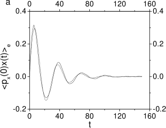
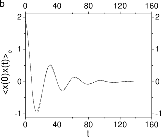
Figure 1: Correlation functions for the NS for $E_{c}=0.38$: (a) $\langle p_{x}(0)x(t)\rangle_{e}$; (b) $\langle x(0)x(t)\rangle_{e}$. The full line shows the numerical results and the dashed line shows the fitting. The averages were computed using 35000 initial conditions.

The correlation functions $\langle p_{x}(0)x(t)\rangle_{e}$ and $\langle x(0)x(t)\rangle_{e}$ are obtained numerically with a fixed time step symplectic integration algorithm forest applied to the isolated chaotic system. Fig. 1 shows the numerical correlation functions for $E_{c}(0)=0.38$. These numerical results can be well fitted by the expressions

$$\begin{array}[]{ll}\langle x(0)x(t)\rangle_{e}&=\sigma e^{-\alpha t}\cos{\omega t},\\ \langle p_{x}(0)x(t)\rangle_{e}&=\mu e^{-\beta t}\sin{\Omega t},\end{array}$$ (17)

with decay rates $\alpha=0.0418$ and $\beta=0.0456$, amplitudes $\sigma=1.865$ and $\mu=0.409$ and frequencies of oscillation $\omega=0.1963$ and $\Omega=0.2043$ with $\chi^{2}\,\sim\,10^{-4}$ (see Fig.1). Notice that the exponents $\alpha$ and $\beta$ and the frequencies $\omega$ and $\Omega$ are very similar. If the interacting system were integrable, these functions would exhibit quasi-periodic oscillations.

Considering the expressions (17) and assuming $\Omega\approx\omega$ and $\beta\approx\alpha$, we obtain the following result for $\langle E_{o}(t)\rangle$

$$\langle E_{o}(t)\rangle=E_{o}(0)+\frac{\gamma^{2}}{m}(B+At+f(t)+g(t)),$$ (18)

where $B$ is a constant, $f(t)$ is an oscillatory function and $g(t)$ is proportional to $e^{-\alpha t}$. The important result is the coefficient $A$

$$A=4\mu\omega\alpha\frac{\left[\frac{\sigma}{4\mu\omega}(\omega^{2}_{0}+\omega^{2}+\alpha^{2})-\frac{E_{o}(0)}{E_{c}(0)}\right]}{[(\omega_{0}-\omega)^{2}+\alpha^{2}][(\omega_{0}+\omega)^{2}+\alpha^{2}]}.$$ (19)

For fixed oscillator frequency $\omega_{0}$ and a given chaotic energy shell $E_{c}(0)$ (and, consequently, for given $\sigma$, $\mu$, $\omega$ and $\alpha$), the ratio $E_{o}(0)/E_{c}(0)$ is the responsible for the average increase or decrease of $\langle E_{o}(t)\rangle$. The short time equilibrium in the energy flow is given by the condition $A=0$, or

$$\frac{E_{o}(0)}{E_{c}(0)}=\frac{\sigma}{4\mu\omega}(\omega^{2}_{0}+\omega^{2}+\alpha^{2})\;.$$ (20)

The equation of motion of $z(t)$ under the average effect of the interaction with the chaotic system can also be written in terms of the response function as

$$\langle\ddot{z}(t)\rangle+\omega^{2}_{0}\langle z(t)\rangle=-\frac{\gamma}{m}\langle x(t)\rangle=\frac{\gamma^{2}}{m}\int_{0}^{t}\mathrm{d}s\,\phi_{xx}(t-s)\langle z(s)\rangle.$$ (21)

Integrating by parts yields

$$\langle\ddot{z}(t)\rangle+\left(\omega^{2}_{0}-\frac{\gamma^{2}F(0)}{m}\right)\langle z(t)\rangle+\frac{\gamma^{2}}{m}\int_{0}^{t}\mathrm{d}s\,F(t-s)\langle\dot{z}(s)\rangle+\frac{\gamma^{2}}{m}z(0)F(t)=0,$$ (22)

where

$$F(t-s)=\int\mathrm{d}s\,\phi_{xx}(t-s)=\frac{2\mu e^{-\alpha(t-s)}}{E_{c}(0)(\alpha^{2}+\omega^{2})}\{\omega\cos{[\omega(t-s)]}+\alpha\sin{[\omega(t-s)]}\}.$$ (23)

Eq.(22) shows that the interaction produces a harmonic correction to the original potential, a dissipative term with memory and an external force proportional to $z(0)$. The choice $z(0)=0$ simplifies (22) and turns it into an average Langevin equation.

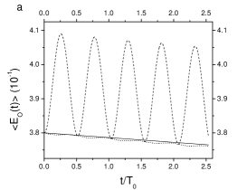
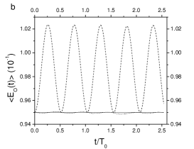
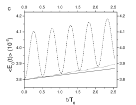
Figure 2: Average oscillator energy at short times with the NS as chaotic system. $T_{0}=1/\omega_{0}$. The dashed line shows $\langle E_{o}(t)\rangle$ and the doted line shows $\langle E_{or}(t)\rangle$, both obtained numerically. The full line shows Eq.(18) without $f(t)$. (a) $E_{o}(0)/E_{c}(0)=1.0$, (b) $E_{o}(0)/E_{c}(0)=0.25$ and (c) $E_{o}(0)/E_{c}(0)=0.1$. The oscillator’s parameters, coupling constant and number of initial conditions are the same as in Fig.2.

Fig.2 shows a comparison between the numerically calculated ‘bare’ oscillator energy $\langle E_{o}(t)\rangle$, where

$$E_{o}(z)=\frac{p_{z}^{2}}{2m}+\frac{m\omega_{0}^{2}z^{2}}{2},$$ (24)

the ‘re-normalized’ oscillator energy $\langle E_{or}(t)\rangle$, where

$$E_{or}(z)=\frac{p_{z}^{2}}{2m}+\frac{m\omega_{0}^{2}z^{2}}{2}-\frac{\gamma^{2}}{2}F(0)z^{2},$$ (25)

and the expression (18) without the oscillating term $f(t)$. We have chosen $\gamma$ and $m$ so that $\omega^{2}_{0}-\gamma^{2}F(0)/m>0$. We also have chosen $\omega_{0}$ so that $e^{-\alpha/\omega_{0}}\approx 10^{-4}$ and $g(t)$ decreases very fast. In this case only the linear and the oscillating terms in Eq.(18) are important. We have subtracted the oscillating part of Eq.(18) in Fig.2 to highlight the linear increase or decrease in the average energy. In the time scale of Fig.2, which corresponds to several periods of the decoupled oscillator, the linear behavior describes very well the numerical results. Fig.2(b) shows the equilibrium situation according to Eq.(20). Notice that $F(t)$ decays very fast in the time scale $1/\omega_{0}$, leading to the dissipative force in Eq.(22).

In the next sections we consider the quantum counterpart of these classical calculations. The chaotic system will be treated semiclassically and the quantum versions of the response and correlation functions will play important roles.

III Quantum Formulation

III.1 The Feynman-Vernon Approach

In this section we describe the dynamics of the coupled oscillator from a quantum point of view. In order to do that we need, like in the classical case, a systematic way to eliminate the detailed information we don’t need about the chaotic system. We will do that using the Feynman-Vernon approach feynman1 . Because of the non-linear chaotic system, we will not be able to perform exact calculations. Instead, we will resort to semiclassical approximations.

We consider the quantum version of the full Hamiltonian, Eq.(1), and again we denote by $q=(x,y)$ the pair of coordinates of the chaotic system. The density matrix operator can be written as

$$\hat{\rho}(T)=|\psi(T)\rangle\langle\psi(T)|=e^{-i\hat{H}T/\hbar}|\psi(0)\rangle\langle\psi(0)|e^{i\hat{H}T/\hbar}$$

where $\psi(T)$ is the wave function of the whole system. In the position representation

$$\rho(z(T),q(T),z^{\prime}(T),q^{\prime}(T))=\langle z,q|\psi(T)\rangle\langle\psi(T)|z^{\prime},q^{\prime}\rangle$$ (26)

$$= \int\mathrm{d}z(0)\mathrm{d}z^{\prime}(0)\mathrm{d}q(0)\mathrm{d}q^{\prime}(0)\langle z,q|e^{-i\hat{H}T/\hbar}|z(0),q(0)\rangle\langle z(0),q(0)|\psi(0)\rangle\times$$

$$\langle\psi(0)|z^{\prime}(0),q^{\prime}(0)\rangle\langle z^{\prime}(0),q^{\prime}(0)|e^{i\hat{H}T/\hbar}|z^{\prime},q^{\prime}\rangle$$

$$= \int\mathrm{d}z(0)\mathrm{d}z^{\prime}(0)\mathrm{d}q(0)\mathrm{d}q^{\prime}(0)K(z(T),q(T),z(0),q(0))\psi(z(0),q(0))\times$$

$$K^{*}(z^{\prime}(T),q^{\prime}(T),z^{\prime}(0),q^{\prime}(0))\psi^{*}(z^{\prime}(0),q^{\prime}(0)),$$

where the propagators can be written in terms of Feynman path integrals as feynman2

$$K(z(T),q(T),z(0),q(0))=\int\mathrm{D}z(t)\mathrm{D}q(t)\exp{\left[\frac{i}{\hbar}S[z(t),q(t)]\right]},$$ (27)

with action

$$S[z(t),q(t)] = \int_{0}^{T}\mathrm{d}t(L_{0}(z(t))+L_{c}(q(t))+L_{I}(z(t),q(t)))$$ (28)

$$\equiv S_{o}+S_{c}+S_{I}.$$

Thus,

$$\rho(z(T),q(T),z^{\prime}(T),q^{\prime}(T))=$$ (29)

$$= \int\mathrm{d}z(0)\mathrm{d}z^{\prime}(0)\mathrm{d}q(0)\mathrm{d}q^{\prime}(0)\mathrm{D}z(t)\mathrm{D}z^{\prime}(t)\mathrm{D}q(t)\mathrm{D}q^{\prime}(t)$$

$$\exp\left[\frac{i}{\hbar}\left(S[z(t),q(t)]-S[z^{\prime}(t),q^{\prime}(t)]\right)\right]\rho(z(0),q(0),z^{\prime}(0),q^{\prime}(0)),$$

where

$$\rho(z(0),q(0),z^{\prime}(0),q^{\prime}(0))=\psi(z(0),q(0))\psi^{*}(z^{\prime}(0),q^{\prime}(0))$$ (30)

is the initial state. As usual we use $z(T)$ and $q(T)$ just as labels for the positions $z$ and $q$ at $T$. $z(T)$ and $q(T)$ are not functions of $T$.

We assume that the initial state can be written as

$$\rho(z(0),q(0),z^{\prime}(0),q^{\prime}(0))=\rho_{o}(z(0),z^{\prime}(0))\rho_{c}(q(0),q^{\prime}(0))$$ (31)

and define the reduced density matrix by

$$\rho_{o}(z(T),z^{\prime}(T))=\int\mathrm{d}q(T)\rho(z(T),q(T),z^{\prime}(T),q(T)).$$ (32)

We obtain

$$\rho_{o}(z(T),z^{\prime}(T))=\int\mathrm{d}z(0)\mathrm{d}z^{\prime}(0)\mathrm{D}z(t)\mathrm{D}z^{\prime}(t)$$ (33)

$$\left\{\int\mathrm{d}q(0)\mathrm{d}q^{\prime}(0)\mathrm{d}q(T)\mathrm{d}q^{\prime}(T)\mathrm{D}q(t)\mathrm{D}q^{\prime}(t)\delta(q(T)-q^{\prime}(T))\right.$$

$$\exp{\left[\frac{i}{\hbar}(S_{c}[q(t)]-S_{c}[q^{\prime}(t)]+S_{I}[z(t),q(t)]-S_{I}[z^{\prime}(t),q^{\prime}(t)\right]}$$

$$\rho_{c}(q(0),q^{\prime}(0))\bigg{\}}\exp{\left[\frac{i}{\hbar}\left(S_{o}[z(t)]-S_{o}[z^{\prime}(t)]\right)\right]\rho_{o}(z(0),z^{\prime}(0))},$$

which can be written as

$$\rho_{o}(z(T),z^{\prime}(T))=\int\mathrm{d}z(0)\mathrm{d}z^{\prime}(0)J(z(T),z^{\prime}(T),z(0),z^{\prime}(0))\rho_{o}(z(0),z^{\prime}(0)),$$ (34)

where

$$J(z(T),z^{\prime}(T),z(0),z^{\prime}(0))=\int\mathrm{D}z(t)\mathrm{D}z^{\prime}(t)\mathcal{F}[z(t),z^{\prime}(t)]\exp[\frac{i}{\hbar}(S_{o}[z(t)]-S_{o}[z^{\prime}(t)])]$$ (35)

is the ‘superpropagator’ and

$$\mathcal{F}[z(t),z^{\prime}(t)]=\int\mathrm{d}q(0)\mathrm{d}q^{\prime}(0)\mathrm{d}q(T)\mathrm{d}q^{\prime}(T)\mathrm{D}q(t)\mathrm{D}q^{\prime}(t)\delta(q(T)-q^{\prime}(T))$$ (36)

$$\exp\left[\frac{i}{\hbar}\left(S_{c}[q(t)]-S_{c}[q^{\prime}(t)]+S_{I}[z(t),q(t)]-S_{I}[z^{\prime}(t),q^{\prime}(t)]\right)\right]\;\rho_{c}(q(0),q^{\prime}(0)),$$

is the so called ‘influence functional’, which contains all the information about the chaotic system.

Equation (34) is the equation of motion for the reduced density matrix. For $\mathcal{F}=1$, $J$ becomes the propagator of the isolated oscillator. Our goal is to get an approximate expression for $J$ that includes the effects of the chaotic system.

We take as the initial state for the chaotic system one of its energy eigenstate $\phi_{a}(q)=\langle q|a\rangle$. Thus,

$$\rho_{c}(q(0),q^{\prime}(0))=\phi_{a}(q(0))\phi_{a}^{*}(q^{\prime}(0)).$$ (37)

This is the quantum version of the classical microcanonical distribution we considered in section II.

The difficulty in the calculation of $J$ is that the chaotic Lagrangian $L_{c}$ is not quadratic. Therefore, $\mathcal{F}$ has to be treated in a perturbative manner. Rewriting $\mathcal{F}$ as

$$\mathcal{F}[z(t),z^{\prime}(t)]=\int\mathrm{d}q(0)\ldots\mathrm{D}q^{\prime}(t)\delta(q(T)-q^{\prime}(T))\exp\left[\frac{i}{\hbar}(S_{c}[q(t)]-S_{c}[q^{\prime}(t)])\right]$$ (38)

$$\exp\left[-\gamma\frac{i}{\hbar}\left(\int_{0}^{T}\mathrm{d}t(z(t)x(t)-z^{\prime}(t)x^{\prime}(t))\right)\right]\phi_{a}(q(0))\phi_{a}^{*}(q^{\prime}(0))$$

we assume that $\gamma$ is small enough so that the exponential in the second line can be expanded to second order in its argument. These terms can be calculated by inserting complete sets of energy eigenstates of $H_{c}$. The result, following feynman1 , is

$$\mathcal{F}[z(t),z^{\prime}(t)]\approx 1-\left(\frac{i\gamma}{\hbar}\right)x_{aa}\int_{0}^{T}\mathrm{d}t[z(t)-z^{\prime}(t)]$$ (39)

$$-\left(\frac{\gamma^{2}}{\hbar}\right)\int_{0}^{T}\mathrm{d}t\int_{0}^{t}\mathrm{d}s[z(t)-z^{\prime}(t)][z(s)F_{a}^{*}(t-s)-z^{\prime}(s)F_{a}(t-s)],$$

where

$$F_{a}(t-s)=\sum_{b}\frac{|x_{ba}|^{2}}{\hbar}\exp[i\omega_{ba}(t-s)],\qquad\omega_{ba}=\frac{E_{b}-E_{a}}{\hbar},$$ (40)

$$x_{ba}=\int\mathrm{d}q\phi_{b}^{*}(q)x\phi_{a}(q),$$ (41)

and $E_{b}$ are the eigen-energies of chaotic system ($x$ is the coordinate of $H_{c}$ in $V_{I}$ ). For the NS $H_{c}(-x)=H_{c}(x)$ and $x_{aa}=0$. Thus,

$$\mathcal{F}[z(t),z^{\prime}(t)]\approx 1-\frac{1}{\hbar}\Phi[z(t),z^{\prime}(t)]\approx\exp\left[-\frac{1}{\hbar}\Phi[z(t),z^{\prime}(t)]\right]$$ (42)

where

$$\Phi[z,z^{\prime}]=\frac{\gamma^{2}}{\hbar}\int_{0}^{T}\mathrm{d}t\int_{0}^{t}\mathrm{d}s[z(t)-z^{\prime}(t)][z(s)F_{a}^{*}(t-s)-z^{\prime}(s)F_{a}(t-s)].$$ (43)

With these approximations the superpropagator can be written as

$$J(z(T),z^{\prime}(T),z(0),z^{\prime}(0))=\int\mathrm{D}z(t)\mathrm{D}z^{\prime}(t)\,e^{\frac{i}{\hbar}(\tilde{S}_{ef}[z(t),z^{\prime}(t)])},$$ (44)

where we have defined the effective action

$$\tilde{S}_{ef}[z(t),z^{\prime}(t)]=S_{o}[z(t)]-S_{o}[z^{\prime}(t)]+i\Phi[z(t),z^{\prime}(t)].$$ (45)

Since $\tilde{S}_{ef}$ is quadratic in $z$ and $z^{\prime}$ the path integral can be solved exactly by the stationary phase method. It is convenient to define the new variables $r(t)=(z(t)+z^{\prime}(t))/2$ and $y(t)=z(t)-z^{\prime}(t)$ weiss and to separate $F_{a}(t)=F_{a}^{{}^{\prime}}(t)+iF_{a}^{{}^{\prime\prime}}(t)$ into real and imaginary parts. This allows us to write

$$J(r(T),y(T),r(0),y(0))=\int\mathrm{D}r(t)\mathrm{D}y(t)\,e^{\frac{i}{\hbar}\tilde{S}[r(t),y(t)]\,-\,\frac{1}{\hbar}\phi[r(t),y(t)]}.$$ (46)

where

$$\tilde{S}[r(t),y(t)]\equiv\int_{0}^{T}\mathrm{d}t\left\{m[\dot{r}(t)\dot{y}(t)-\omega_{0}^{2}r(t)y(t)]+2\gamma^{2}y(t)\int_{0}^{t}\mathrm{d}sF_{a}^{{}^{\prime\prime}}(t-s)r(s)\right\},$$ (47)

and

$$\phi[r(t),y(t)]\equiv\gamma^{2}\int_{0}^{T}\mathrm{d}t\int_{0}^{t}\mathrm{d}sy(t)y(s)F_{a}^{{}^{\prime}}(t-s),$$ (48)

are the real and imaginary parts of $\tilde{S}_{ef}$. In Appendix A we show that

$$J(r(T),y(T),r(0),y(0))=G(T,0)\exp\left\{\frac{i}{\hbar}\tilde{S}[r_{e},y_{e}]\right\}\exp\left\{-\frac{1}{\hbar}\phi[y_{e},y_{e}]\right\},$$ (49)

where $G(T,0)$ can be obtained by the normalization condition of reduced density matrix and $r_{e}(t)$ and $y_{e}(t)$ are the extremum paths of $\tilde{S}$, which satisfy

$$\ddot{r}_{e}(t)+\omega_{0}^{2}r_{e}(t)-\frac{2\gamma^{2}}{m}\int_{0}^{t}\mathrm{d}sF_{a}{{}^{\prime\prime}}(t-s)r_{e}(s)=0,$$ (50)

$$\ddot{y}_{e}(t)+\omega_{0}^{2}y_{e}(t)-\frac{2\gamma^{2}}{m}\int_{0}^{t}\mathrm{d}sF_{a}{{}^{\prime\prime}}(s-t)y_{e}(s)=0.$$ (51)

Therefore we need $F_{a}^{{}^{\prime\prime}}$ to solve (50) and (51) and we also need $F_{a}^{{}^{\prime}}$ to calculate $\phi[y_{e},y_{e}]$.

From Eq.(40) it follows that

$$F_{a}(t)=\frac{\langle a|\hat{x}(0)\hat{x}(t)|a\rangle}{\hbar},$$ (52)

where $\hat{x}(t)$ is the Heisenberg representation of $\hat{x}$. The real and imaginary parts of $F_{a}$ are

$$F_{a}^{{}^{\prime}}(t)=\frac{\langle a|\{\hat{x}(0),\hat{x}(t)\}|a\rangle}{2\hbar},$$ (53)

and

$$F_{a}^{{}^{\prime\prime}}(t)=\frac{\langle a|[\hat{x}(0),\hat{x}(t)]|a\rangle}{2i\hbar},$$ (54)

where $\{.\}$ is the anticomutator and $[.]$ is the comutator. Thus, $F_{a}^{{}^{\prime}}$ and $F_{a}^{{}^{\prime\prime}}$ are, respectively, the quantum analogs of the classical correlation and response functions of Section II.

III.2 Semiclassical Expressions for Correlation Functions.

In this section we obtain semiclassical formulas for $F_{a}^{{}^{\prime}}(t)$ and $F_{a}^{{}^{\prime\prime}}(t)$. We write

$$F_{a}^{{}^{\prime}}(t)=\frac{1}{2\hbar}\sum_{b}\langle b|\{\hat{x}(0),\hat{x}(t)\}\hat{\rho}|b\rangle=\frac{1}{2\hbar}Tr(\hat{f}(t)\hat{\rho}),$$ (55)

where $\hat{\rho}=|a\rangle\langle a|$ is the microcanonical distribution of the chaotic system and $\hat{f}=\{\hat{x}(0),\hat{x}(t)\}$. To calculate $F^{\prime\prime}_{a}$ we take $\hat{f}=-i[\hat{x}(0),\hat{x}(t)]$. Using the Wigner-Weyl representation wigner the trace can be written as

$$Tr[\hat{f}(t)\hat{\rho}]=\int\frac{\mathrm{d}^{2}q\mathrm{d}^{2}p}{(2\pi\hbar)^{2}}f(q,p;t)W(q,p)$$ (56)

where

$$f(q,p;t)=\int_{-\infty}^{\infty}\mathrm{d}u\,e^{\frac{i}{\hbar}p\cdot u}\langle q-u/2|\hat{f}(t)|q+u/2\rangle.$$ (57)

is the Weyl transformation (or symbol) of $\hat{f}(t)$ and $W(q,p)$ is the Wigner function of $\hat{\rho}$. For $\hat{f}(t)=-i[\hat{x}(0),\hat{x}(t)]$ we have

$$f(q,p;t) = -i\int_{-\infty}^{\infty}\mathrm{d}u\,e^{ip\cdot u/\hbar}\,\langle q-u/2|(\hat{x}\hat{x}(t)-\hat{x}(t)\hat{x})|q+u/2\rangle$$ (58)

$$= -i\int_{-\infty}^{\infty}\mathrm{d}u\,e^{ip\cdot u/\hbar}\,(-u_{x})\langle q-u/2|\hat{x}(t)|q+u/2\rangle$$

$$= \hbar\frac{\partial}{\partial p_{x}}\left\{\int_{-\infty}^{\infty}\mathrm{d}u\,e^{ip\cdot u/\hbar}\,\langle q-u/2|\hat{x}(t)|q+u/2\rangle\right\}$$

$$= \hbar\frac{\partial}{\partial p_{x}}\left\{\int_{-\infty}^{\infty}\mathrm{d}u\,e^{ip\cdot u/\hbar}\,\int_{-\infty}^{\infty}\mathrm{d}v\,v_{x}K^{*}(v,q-u/2;t)K(v,q+u/2;t)\right\}$$

where $u$ and $v$ represent coordinates of the chaotic system and $K(v,v^{\prime};t)=\langle v|e^{-i\hat{H}_{c}t/\hbar}|v^{\prime}\rangle$ is the propagator.

We now replace the propagators by their semiclassical expressions $\tilde{K}$ and do the integrals by the stationary phase approximation. The stationary phase condition shows that the most important contributions come from the trajectories starting at $q-u/2$ (for $K^{*}$) and $q+u/2$ (for $K$) and arriving at $v$ in the time $t$ such that

$$\nabla_{v}R_{k}(v,q-u/2)-\nabla_{v}R_{l}(v,q+u/2)=0,$$ (59)

where $R_{k}$ and $R_{l}$ are Hamilton’s principal functions coming from the phases in $\tilde{K}$ and $\tilde{K}^{*}$. Since $\nabla_{v}R_{i}(v,v^{\prime})$ gives the final momentum, (59) imposes that the final momenta of the two trajectories must be equal. Since the final positions are also equal, the two trajectories must be identical. Thus,

$$\int_{-\infty}^{\infty}\mathrm{d}v\,v_{x}\tilde{K}^{*}(v,q-u/2;t)\tilde{K}(v,q+u/2;t)\approx x(q,p;t)\delta(u),$$ (60)

where $x(q,p;t)$ is the coordinate $x$ of the stationary trajectory.

Using (60) in (58) we find

$$f(q,p;t)=\hbar\frac{\partial}{\partial p_{x}}x(q,p;t)=\hbar\{x(0),x(t)\}.$$ (61)

since

$$\{x(0),x(t)\}=\frac{\partial x(0)}{\partial x(0)}\frac{\partial x(t)}{\partial p_{x}(0)}-\frac{\partial x(0)}{\partial p_{x}(0)}\frac{\partial x(t)}{\partial x(0)}=\frac{\partial x(t)}{\partial p_{x}(0)}.$$ (62)

For $\hat{f}(t)=\{\hat{x}(0),\hat{x}(t)\}$, we find

$$f(q,p;t) = \int_{-\infty}^{\infty}\mathrm{d}u\exp\left(\frac{i}{\hbar}p\cdot u\right)2q_{x}\langle q-u/2|\hat{X}(t)|q+u/2\rangle$$ (63)

$$\approx 2q_{x}\,x(q,p;t)=2x(0)x(t).$$

The semiclassical limit of the Wigner function

$$W(q,p;E)=\frac{1}{\hbar}\int_{-\infty}^{\infty}\mathrm{d}te^{iEt/\hbar}\int\mathrm{d}u\exp\left(\frac{i}{\hbar}p\cdot u\right)K(q+u/2,q-u/2;t).$$ (64)

was obtained by Berry berry2 and can be written as

$$W(q,p;E)\approx\delta(E-H(q,p))+W_{1}(q,p;E).$$ (65)

The first term is the classical micro-canonical distribution and the second, $W_{1}$, is given by classical periodic orbits corrections to the classical function. These periodic orbits have energy $E=E_{a}$, corresponding to the eigenstate $|a\rangle$ of the microcanonical quantum distribution. Using (65) we write

$$Tr[\hat{f}(t)\hat{\rho}] \approx\displaystyle{\frac{1}{(2\pi\hbar)^{2}}} \left[\int\mathrm{d}q\mathrm{d}pf(q,p;t)\delta(E-H(q,p))\,+\int\mathrm{d}q\mathrm{d}pf(q,p;t)W_{1}(q,p;E)\right]$$ (66)

$$\equiv\frac{1}{(2\pi\hbar)^{2}}\left[f^{0}+f^{1}\right].$$

When $f(q,p;t)$ is replaced by the semiclassical expressions for the anticomutator and comutator, the first term of (66) becomes, except for a normalization, the classical expressions for the response and correlation functions respectively. Following berry2 the second term of (66) becomes

$$f^{1}(E,t)\approx\sum_{j}A_{j}\cos{(S_{j}(E)/\hbar+\gamma_{j})}\oint\mathrm{d}\tau f(q_{j}(\tau),p_{j}(\tau);t).$$ (67)

where, $A_{j}$ depends on the stability of $j$-periodic orbit, $S_{j}(E)$ is its action, $\gamma_{j}$ is the Maslov index and the integral is calculated over a period of the $j$-orbit. Analogous results can be found, for example, in eckart .

Furthermore berry2 ,

$$\begin{array}[]{ll}Tr(\hat{\rho})&=\displaystyle{\frac{1}{(2\pi\hbar)^{2}}}\left[\int\mathrm{d}q\mathrm{d}p\,\delta(E-H(q,p))+n_{q}(E;\hbar)\right]\\ \\ &=\displaystyle{\frac{1}{(2\pi\hbar)^{2}}}[n_{c}(E)+n_{q}(E;\hbar)]\\ \end{array}$$ (68)

where the first term is the classical density of states and the second term is known as Gutzwiller’s trace formula. Thus,

$$\begin{array}[]{ll}\displaystyle{\frac{Tr[\hat{f}(t)\hat{\rho}]}{Tr[\hat{\rho}]}}&\approx\displaystyle{\frac{f^{0}(E;t)+f^{1}(E;t)}{n_{c}(E)+n_{q}(E;\hbar)}}\\ \\ &\approx\langle f(q,p;t)\rangle_{cl.}\left[1-\frac{n_{q}(E;\hbar)}{n_{c}(E)}\right]+\frac{f^{1}(E;t)}{n_{c}(E)}\left[1-\frac{n_{q}(E;\hbar)}{n_{c}(E)}\right]\end{array}$$ (69)

where $\langle f(q,p;t)\rangle_{cl.}=f^{0}(E,t)/n_{c}(E)$.

Finally, we can calculate the semiclassical expressions for $F_{a}^{{}^{\prime\prime}}(t)$ and $F_{a}^{{}^{\prime}}(t)$. From (61), (63) and (69)

$$F_{a}^{{}^{\prime}}(t) \approx \frac{\langle x(0)x(t)\rangle_{cl.}}{\hbar}\left[1-\frac{n_{q}(E;\hbar)}{n_{c}(E)}\right]$$ (70)

$$+ \frac{1}{\hbar n_{c}(E)}\sum_{j}A_{j}\cos\left(S_{j}(E)/\hbar+\gamma_{j}\right)\oint\mathrm{d}\tau x_{j}(\tau)x_{j}(\tau+t).$$

and

$$F_{a}^{{}^{\prime\prime}}(t)=\frac{\langle\hat{O}(t)\rangle}{2\hbar} \approx \frac{\langle\{x(0),x(t)\}\rangle_{cl.}}{2}\left[1-\frac{n_{q}(E;\hbar)}{n_{c}(E)}\right]$$

$$+ \frac{1}{2n_{c}(E)}\sum_{j}A_{j}\cos\left(S_{j}(E)/\hbar+\gamma_{j}\right)\oint\mathrm{d}\tau\{x_{j}(\tau),x_{j}(\tau+t)\}.$$

(71)

Both these semiclassical expressions are given by their classical counterparts multiplied by a correction to their amplitudes, given by $n_{q}(E;\hbar)/n_{c}(E)$, plus a correction from periodic orbits. The temporal dependence of the first is given solely by the classical dynamics and it decays exponentially. The second term, however, is a sum of oscillating functions and carries the temporal dependence characteristic of the chaotic system. As a final remark we note in esposito1 these functions were calculated using random matrix theory.

III.3 The Superpropagator

The semiclassical expressions for $F_{a}^{{}^{\prime}}(t)$ and $F_{a}^{{}^{\prime\prime}}(t)$ allows us to solve the equations of motion (50) and (51) and to calculate the superpropagator, Eq.(49). In order to have explicit formula, we shall consider only the zero order approximation $F_{a}^{{}^{\prime\prime}}(t)\approx\phi_{xx}(t)/2$. Substituting it in (50) and (51) and integrating by parts we get

$$\ddot{r}_{e}(t)+\Omega^{2}_{0}\,r_{e}(t)+\frac{\gamma^{2}}{m}\int_{0}^{t}\mathrm{d}sF(t-s)\dot{r}_{e}(s) = -\frac{\gamma^{2}}{m}r_{e}(0)F(t),$$ (72)

$$\ddot{y}_{e}(t)+\chi^{2}_{0}\,y_{e}(t)-\frac{\gamma^{2}}{m}\int_{0}^{t}\mathrm{d}sF(t-s)\dot{y}_{e}(s) = \frac{\gamma^{2}}{m}y_{e}(0)F(t),$$ (73)

where $\Omega_{0}^{2}=\omega_{0}^{2}-\gamma^{2}F(0)/m$, $\chi^{2}_{0}=\omega_{0}^{2}+\gamma^{2}F(0)/m$ and

$$F(t)=\int\mathrm{d}s\phi_{xx}(t-s),$$ (74)

as in the classical case (eq.(23)).

In Appendix B we solve these equations by the method of Laplace transforms. We find that the solutions involve two very different time scales. The shortest time scale is relevant only for times much smaller than $1/\omega_{0}$, the period of the decoupled oscillator. For times of the order of $1/\omega_{0}$ these terms can be discarded as transients. Here we shall adopt this approximation and keep only the terms that are significant for times of $1/\omega_{0}$. In this case we show that (72) and (73) can be written as

$$\ddot{r}_{e}(t)+2\Lambda\dot{r}_{e}(t)+\Omega_{0}^{2}r_{e}(t)=0,\quad\Omega_{0}^{2}\gg\Lambda^{2},$$ (75)

$$\ddot{y}_{e}(t)-2\Lambda\dot{y}_{e}(t)+\chi_{0}^{2}y_{e}(t)=0,\quad\chi_{0}^{2}\gg\Lambda^{2},$$ (76)

where

$$\Lambda=\frac{\gamma^{2}}{2m}\lim_{t\to\infty}\int_{0}^{t}\mathrm{d}sF(t-s).$$ (77)

Approximating $\Omega_{0}\approx\chi_{0}\approx\omega_{0}$ we find

$$r_{e}(t)=e^{-\Lambda t}\left\{\frac{\sin{[\omega_{0}(T-t)]}}{\sin{(\omega_{0}T)}}r(0)+e^{\Lambda T}\frac{\sin{(\omega_{0}t)}}{\sin{(\omega_{0}T)}}r(T)\right\},$$

$$y_{e}(t)=e^{\Lambda t}\left\{\frac{\sin{[\omega_{0}(T-t)]}}{\sin{(\omega_{0}T)}}y(0)+e^{-\Lambda T}\frac{\sin{(\omega_{0}t)}}{\sin{(\omega_{0}T)}}y(T)\right\}.$$ (78)

Within this approximation we can calculate the real part $\tilde{S}$ of the effective action, Eq.(47). We obtain

$$\tilde{S}[r_{e},y_{e}] = [m\omega_{0}^{2}K(T)-m\Lambda]r(T)y(T)+[m\omega_{0}^{2}K(T)+m\Lambda]r(0)y(0)$$ (79)

$$-m\omega_{0}^{2}L(T)r(0)y(T)-m\omega_{0}^{2}N(T)r(T)y(0),$$

where,

$$K(T) = \frac{1}{\omega_{0}}\frac{\cos(\omega_{0}T)}{\sin(\omega_{0}T)},$$ (80)

$$L(T) = \frac{1}{\omega_{0}}\frac{e^{-\Lambda T}}{\sin(\omega_{0}T)},$$ (81)

$$N(T) = \frac{1}{\omega_{0}}\frac{e^{\Lambda T}}{\sin(\omega_{0}T)}.$$ (82)

For the imaginary part $\phi$ of the effective action, Eq.(48), we get

$$\phi[y_{e},y_{e}]=\gamma^{2}\int_{0}^{T}\mathrm{d}t\,y_{e}(t)\int_{0}^{t}\mathrm{d}s\,F_{a}^{{}^{\prime}}(t-s)y_{e}(s).$$ (83)

Using again only the zero order term of the semiclassical expression (70) for $F_{a}^{{}^{\prime}}(t)$ and the fact that the classical correlation function decays exponentially, as in (77), we can approximate, for $t\sim 1/\omega_{0}$

$$\int_{0}^{t}\mathrm{d}s\,F_{a}^{{}^{\prime}}(t-s)y_{e}(s)\approx y_{e}(t)\lim_{t\to\infty}\int_{0}^{t}\mathrm{d}s\,F_{a}^{{}^{\prime}}(t-s)\equiv y_{e}(t)\frac{B^{\prime}}{\hbar},$$ (84)

which implies that

$$\begin{array}[]{ll}\phi[y_{e},y_{e}]&=\displaystyle{\frac{\gamma^{2}B^{\prime}}{\hbar}}\int_{0}^{T}\mathrm{d}t\,y^{2}_{e}(t)\\ &=\displaystyle{\frac{\gamma^{2}B^{\prime}}{\hbar}}[A(T)y^{2}(T)+B(T)y(T)y(0)+C(T)y^{2}(0)],\end{array}$$ (85)

where

$$A(T) = \frac{[-\omega_{0}^{2}e^{-2\Lambda T}+(\Lambda^{2}+\omega_{0}^{2})-\Lambda^{2}\cos{(2\omega_{0}T)-\Lambda\omega_{0}\sin{(2\omega_{0}T)}}]}{4\Lambda(\omega_{0}^{2}+\Lambda^{2})\sin^{2}{(\omega_{0}T)}},$$ (86)

$$B(T) = \frac{[-\omega_{0}^{2}\sinh{(\Lambda T)}\cos{(\omega_{0}T)}+\Lambda\omega_{0}\cosh{(\Lambda T)}\sin{(\omega_{0}T)}]}{\Lambda(\omega_{0}^{2}+\Lambda^{2})\sin^{2}{(\omega_{0}T)}},$$ (87)

$$C(T) = \frac{[\omega_{0}^{2}e^{2\Lambda T}-(\Lambda^{2}+\omega_{0}^{2})+\Lambda^{2}\cos{(2\omega_{0}T)-\Lambda\omega_{0}\sin{(2\omega_{0}T)}}]}{4\Lambda(\omega_{0}^{2}+\Lambda^{2})\sin^{2}{(\omega_{0}T)}}.$$ (88)

Finally, putting everything together we get

$$J(r(T),y(T),r(0),y(0))=G(T,0)\exp{\left\{\frac{i}{\hbar}\tilde{S}[r_{e},y_{e}]\right\}}\exp{\left\{-\frac{1}{\hbar}\phi[y_{e},y_{e}]\right\}}$$ (89)

$$= G(T,0)\exp{\left\{\frac{i}{\hbar}\tilde{K}_{2}(T)r(T)y(T)\right\}}\exp{\left\{-\frac{1}{\hbar}\tilde{A}(T)y^{2}(T)\right\}}\times$$

$$\exp{\left\{\frac{i}{\hbar}\left[\tilde{K}_{1}(T)r(0)y(0)-\tilde{L}(T)r(0)y(T)-\tilde{N}(T)r(T)y(0)\right]\right\}}\times$$

$$\exp{\left\{-\frac{1}{\hbar}\tilde{B}(T)y(T)y(0)-\frac{1}{\hbar}\tilde{C}(T)y^{2}(0)\right\}}$$

where

$$\tilde{K}_{1,2}(T)=m\omega_{0}^{2}K(T)\pm m\Lambda\qquad \tilde{L}(T)=m\omega_{0}^{2}L(T) \qquad\tilde{N}(T)=m\omega_{0}^{2}N(T)$$

$$\tilde{A}(T)=\frac{\gamma^{2}B^{\prime}}{\hbar}A(T)\qquad \tilde{B}(T)=\frac{\gamma^{2}B^{\prime}}{\hbar}B(T) \qquad\tilde{C}(T)=\frac{\gamma^{2}B^{\prime}}{\hbar}C(T).$$

(90)

We finish this section with a comment about the physical situation described by these calculations. Since we have considered only the first terms of the semiclassical expressions for $F_{a}^{{}^{\prime}}$ and $F_{a}^{{}^{\prime\prime}}$ our results are valid only in the Ehrenfest time scale of the chaotic system given by beenaker

$$t_{E}\sim\frac{1}{\lambda_{L}}\ln{\left(\frac{S_{c}}{\hbar}\right)},$$ (91)

where $\lambda_{L}$ is the Lyapunov exponent and $S_{c}$ is a typical action of the chaotic system, for example the action of the shortest periodic orbit. Approximating $\lambda_{L}$ by $\alpha$, we see that, in order to observe effects for $t\sim 1/\omega_{0}$, we must have

$$t_{E}\sim\frac{1}{\omega_{0}}=\frac{1}{\alpha}\ln{\left(\frac{S_{c}}{\hbar}\right)}\Rightarrow\frac{S_{c}}{\hbar}=\exp{\left(\frac{\alpha}{\omega_{0}}\right)}.$$ (92)

For NS, $\alpha/\omega_{0}\sim 8$ and $S_{c}\approx 10$ which means that $\hbar$ must be smaller than $10^{-3}$ for our results to be valid.

IV Applications

The superpropagator allows us to study the time evolution of the oscillator under the influence of the chaotic system. The reduced density matrix satisfies

$$\rho_{o}(r(T),y(T))=\int\mathrm{d}r(0)\mathrm{d}y(0)\,J(r(T),y(T),r(0),y(0))\,\rho_{o}(r(0),y(0)).$$ (93)

In the following we calculate explicitly the propagation of two different oscillator’s states. These two applications are similar to the ones presented by Caldeira and Leggett to study dissipation and decoherence.

IV.1 Propagation of a Gaussian State.

For a Gaussian state

$$\psi(z(0))=\frac{1}{(2\pi\sigma^{2})^{1/4}}\,e^{\frac{i}{\hbar}pz(0)/\hbar}e^{-z^{2}(0)/4\sigma^{2}}$$ (94)

the density matrix $\rho_{o}(z(0),z^{\prime}(0))=\psi^{*}(z^{\prime}(0))\psi(z(0))$ can be written in terms of $r=(z+z^{\prime})/2$ and $y=z-z^{\prime}$ as

$$\rho_{o}(r(0),y(0))=\frac{1}{(2\pi\sigma^{2})^{1/2}}\,e^{\frac{i}{\hbar}py(0)}e^{-r^{2}(0)/2\sigma^{2}}e^{-y^{2}(0)/8\sigma^{2}}.$$ (95)

Substituting (89) and (95) in (93) and performing the integrals, we get

$$\rho_{o}(r(T),y(T))=G(T,0)\left[\frac{2\pi\hbar^{2}}{2\hbar\tilde{C}_{1}(T)+\sigma^{2}\tilde{K}_{1}^{2}(T)}\right]^{1/2}$$

$$\times\exp{\left\{-\frac{\tilde{N}^{2}(T)}{2[2\hbar\tilde{C}_{1}(T)+\sigma^{2}\tilde{K}_{1}^{2}(T)]}\left(r(T)-\frac{p}{\tilde{N}(T)}\right)^{2}\right\}}$$

$$\times\exp{\left\{-\left[\frac{\tilde{A}(T)}{\hbar}+\frac{\sigma^{2}\tilde{L}^{2}(T)}{2\hbar^{2}}-\frac{(\sigma^{2}\tilde{K}_{1}(T)\tilde{L}(T)-\hbar\tilde{B}(T))^{2}}{2\hbar^{2}[2\hbar\tilde{C}_{1}(T)+\sigma^{2}\tilde{K}_{1}^{2}(T)]}\right]y^{2}(T)\right\}}$$

$$\times\exp\left\{\frac{i}{\hbar}\tilde{K}_{2}(T)r(T)y(T)-\frac{i}{\hbar}\frac{(\sigma^{2}\tilde{K}_{1}(T)\tilde{L}(T)-\hbar\tilde{B}(T))}{(2\hbar\tilde{C}_{1}(T)+\sigma^{2}\tilde{K}_{1}^{2}(T))}\tilde{N}(T)\left(r(T)-\frac{p}{\tilde{N}(T)}\right)y(T)\right\}$$ ,

where,

$$\tilde{C}_{1}(T)=\tilde{C}(T)+\frac{\hbar}{8\sigma^{2}}.$$ (97)

For $y=z-z^{\prime}=0$, $\rho_{o}$ becomes the probability density. After normalizing we obtain

$$\rho_{o}(r(T),0) = \left[\frac{\tilde{N}^{2}(T)}{2\pi[2\hbar\tilde{C}_{1}(T)+\sigma^{2}\tilde{K}_{1}^{2}(T)]}\right]^{1/2}$$ (98)

$$\times \exp{\left\{-\frac{\tilde{N}^{2}(T)}{2[2\hbar\tilde{C}_{1}(T)+\sigma^{2}\tilde{K}_{1}^{2}(T)]}\left(r(T)-\frac{p}{\tilde{N}(T)}\right)^{2}\right\}}.$$

Eq.(98) represents a Gaussian packet whose center follows the trajectory

$$r(T)=\frac{p}{\tilde{N}(T)}=\frac{p}{m\omega_{0}}e^{-\Lambda T}\sin{(\omega_{0}T)}.$$ (99)

The dissipative effect due to the interaction with the chaotic system is explicit. The same behavior was obtained by Caldeira and Leggett caldeira1 using a thermal bath with many degrees of freedom. Eq.(99) represents the trajectory of a weakly damped harmonic oscillator. The critical and strongly damped cases cannot be described by this formalism because of the weak coupling regime adopted.

The width of the evolved packet is given by

$$\sigma^{2}(T) = \frac{\sigma^{2}\tilde{K}_{1}^{2}(T)+2\hbar\tilde{C}_{1}(T)}{\tilde{N}^{2}(T)}.$$ (100)

After some algebra we can show that

$$\sigma^{2}(T) = \sigma^{2}\bigg{\{}\frac{(1+\epsilon^{2})e^{-2\Lambda T}}{1+\epsilon^{2}}$$ (101)

$$+ \frac{\Gamma[1-e^{-2\Lambda T}(1+2\epsilon\sin{(\omega_{0}T)}\cos{(\omega_{0}T)}+2\epsilon^{2}\sin^{2}{(\omega_{0}T)})]}{1+\epsilon^{2}}\bigg{\}},$$

where

$$\epsilon=\frac{\Lambda}{\omega_{0}}\qquad\mathrm{and}\qquad\Gamma=\frac{E_{c}(0)}{\hbar\omega_{0}}.$$ (102)

The expression above for $\Gamma$ comes from the following considerations: from $\tilde{C}_{1}(T)$ it follows that

$$\Gamma=\frac{\gamma^{2}B^{\prime}}{\hbar m\omega_{0}\Lambda}.$$ (103)

Using Eqs.(77) and (23) and the relation weiss

$$\langle p_{x}(0)x(t)\rangle_{e}=-\frac{\partial}{\partial t}\langle x(0)x(t)\rangle_{e}$$ (104)

we obtain

$$\Lambda=\frac{\gamma^{2}B^{\prime}}{mE_{c}(0)},$$ (105)

which leads directly to (102). Notice that, due to (92), $\Gamma\gg 1$ is the only possibility.

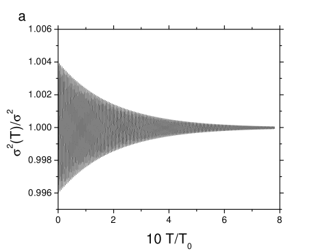
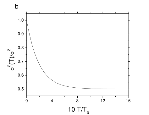
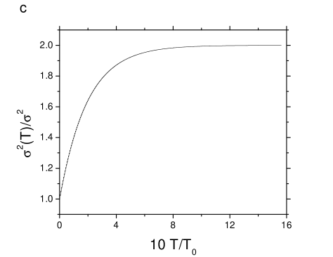
Figure 3: Squared width of wave packet $\sigma^{2}(T)/\sigma^{2}$ as given by Eq.(101) with $T_{0}=1/\omega_{0}$. (a) $\Gamma=1.0$, (b) $\Gamma=0.5$ and (c) $\Gamma=2.0$.

Fig.3 shows that $\sigma^{2}(T)$ for $\Gamma=1$, $0.5$ and $2.0$. These curves can be well fitted by the simpler expression

$$\sigma^{2}(T)=\sigma^{2}[e^{-2\Lambda T}+\Gamma(1-e^{-2\Lambda T})],$$ (106)

which, for $t\sim 1/\omega_{0}$, can be written as

$$\sigma^{2}(T)=\sigma^{2}[1+(\Gamma-1)2\Lambda T].$$ (107)

We see that $\sigma^{2}(\Gamma-1)\Lambda$ plays the role of a diffusion constant. Fig.3 also shows that $\Gamma$ controls the increase or decrease of $\sigma^{2}(T)$. In the present case, $\sigma^{2}(T)$ can only increase because of the constraint $\Gamma\gg 1$. In the Caldeira-Leggett model, on the other hand, the width can also decrease if the the temperature is very low.

IV.2 Superposition of Two Gaussian States.

We now consider an initial state consisting of two Gaussian wave-packets, one at the origin and one centered at $z(0)=q_{0}$:

$$\psi(z(0)) = N^{1/2}[\psi_{1}(z(0))+\psi_{2}(z(0))]$$ (108)

$$= N^{1/2}\left\{\exp{\left[-\frac{z^{2}(0)}{4\sigma^{2}}\right]}+\exp{\left[-\frac{(z(0)-q_{0})^{2}}{4\sigma^{2}}\right]}\right\}.$$

The density matrix is given by

$$\rho_{o}(z(0),z^{\prime}(0))= N [\rho_{11}(z(0),z^{\prime}(0))+\rho_{22}(z(0),z^{\prime}(0))$$ (109)

$$+ \rho_{12}(z(0),z^{\prime}(0))+\rho_{21}(z(0),z^{\prime}(0))].$$

with $\hat{\rho}_{ij}=|\psi_{i}\rangle\langle\psi_{j}|$. The time evolution of $\rho_{o}$ can again be calculated with Eq.(93). The result, for $y=z-z^{\prime}=0$ is

$$\rho_{11}(r(T),0) = \frac{1}{2[1+h(T)]}\left(\frac{\tilde{N}^{2}(T)}{\pi\tilde{f}(T)}\right)^{1/2}\exp{\left\{-\frac{\tilde{N}^{2}(T)}{\tilde{f}(T)}r^{2}(T)\right\}},$$ (110)

$$\rho_{22}(r(T),0) = \frac{1}{2[1+h(T)]}\left(\frac{\tilde{N}^{2}(T)}{\pi\tilde{f}(T)}\right)^{1/2}\exp{\left\{-\frac{\tilde{N}^{2}(T)}{\tilde{f}(T)}\left[r(T)-Q(T)\right]^{2}\right\}},$$ (111)

$$\rho_{12}(r(T),0) + \rho_{21}(r(T),0)\,=$$ (112)

$$\frac{1}{2[1+h(T)]}\left(\frac{\tilde{N}^{2}(T)}{\pi\tilde{f}(T)}\right)^{1/2}\exp{\left[-\frac{q^{2}_{0}}{8\sigma^{2}}g(T)\right]}\exp{\left\{-\frac{\tilde{N}^{2}(T)}{\tilde{f}(T)}r^{2}(T)\right\}}$$

$$\times \exp{\left\{-\frac{\tilde{N}^{2}(T)}{\tilde{f}(T)}\left[r(T)-Q(T)\right]^{2}\right\}}$$

$$\times 2\cos\left\{\frac{\hbar\tilde{N}^{2}(T)}{4\sigma^{2}\tilde{f}(T)\tilde{K}_{1}(T)}\left[\left(r(T)-Q(T)\right)^{2}-r^{2}(T)\right]\right\},$$

where

$$\tilde{f}(T) = 2[2\hbar\tilde{C}_{1}(T)+\sigma^{2}\tilde{K}_{1}^{2}(T)],$$ (113)

$$h(T) = \exp{\left\{-\frac{q^{2}_{0}}{8\sigma^{2}}\left[1+g(T)\right]\right\}},$$ (114)

$$Q(T) = \frac{\tilde{K}_{1}(T)}{\tilde{N}(T)}q_{0},$$ (115)

$$g(T) = \frac{2\hbar\tilde{C}(T)}{2\hbar\tilde{C}_{1}(T)+\sigma^{2}\tilde{K}_{1}^{2}(T)}.$$ (116)

The interference term can also be rewritten as

$$\rho_{12}(r(T),0) + \rho_{21}(r(T),0)=2\cos{\left[a(T)((r(T)-Q(T))^{2}-r^{2}(T))\right]}$$ (117)

$$\times \rho_{1}^{1/2}(r(T),0)\rho_{2}^{1/2}(r(T),0)\exp{\left[-\frac{q^{2}_{0}}{8\sigma^{2}}g(T)\right]}.$$

Eq.(117) shows that the interference is attenuated by $\exp{[-(q^{2}_{0}/8\sigma^{2})g(T)]}$. Eq.(117) is very similar to the expression obtained by Caldeira and Leggett caldeira2 , although there is no temperature dependence in $g(T)$, which can be written as

$$g(T)=\frac{\Gamma\,b(T)}{(1+\epsilon^{2})+\Gamma\,b(T)},$$ (118)

with

$$b(T)=e^{2\Lambda T}-1-2\epsilon\sin{(\omega_{0}T)}\cos{(\omega_{0}T)}-2\epsilon^{2}\sin^{2}{(\omega_{0}T)}$$ (119)

and $\epsilon=\Lambda/\omega_{0}$. We note that the asymptotic limits

$$g(T=0)=0\qquad\mathrm{and}\qquad g(T\rightarrow\infty)\rightarrow 1$$ (120)

are the same as those in the Caldeira-Leggett model.

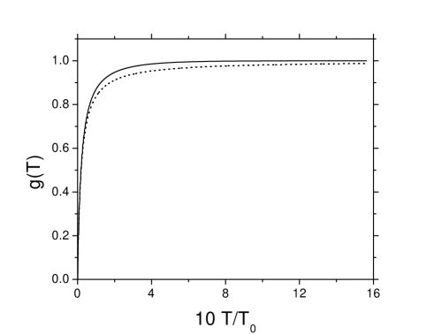
Figure 4: The full line shows $g(T)$ as given by Eq.(118) for $\Gamma=10.0$. $T_{0}=1/\omega_{0}$. The dotted line shows $g(T)$ as given by Eq.(121) for $\Gamma=10.0$.

Fig.4 shows $g(T)$ for $\Gamma=10$. In the regime $\Gamma\gg 1$, we can approximate $g(T)$ by

$$g(T)=\frac{2\Gamma\Lambda T}{1+2\Gamma\Lambda T}.$$ (121)

This simplified expression helps to estimate of the decoherence time. For example, with (121), we can estimate the time $T^{\prime}$ such that

$$\exp{\left[-\frac{q^{2}_{0}}{8\sigma^{2}}g(T^{\prime})\right]}\sim 10^{-3}.$$ (122)

Defining $n\equiv q^{2}_{0}/8\sigma^{2}$ (the number of quanta $\hbar\omega_{0}$ of the wave packet centered at $q_{0}$), we get

$$\left[\frac{n-\ln(10)}{3\ln(10)}\right]2\Gamma\Lambda T^{\prime}=2\tilde{n}\Gamma\Lambda T^{\prime}=1\Rightarrow T^{\prime}=\frac{1}{2\tilde{n}\Gamma\Lambda}.$$ (123)

Since we are interested in the situation where $n\gg 1$ and $\Gamma\gg 1$, we find that the decoherence time is much smaller than the time scale where dissipation takes place, i.e., $T^{\prime}\ll 1/\Lambda$.

V Discussion and Conclusions

We have made two important assumptions in our calculation of the superpropagator. The first of these assumptions, the weak coupling regime, was important to reduce the path integral to a quadratic form in the oscillator variables. The second assumption was the semiclassical regime of the chaotic system. This was essential to establish the connection between the coupling in the influence functional and the classical correlation and response functions that enter in the classical description of the system. The use of these classical functions make the importance of the chaotic dynamics explicit and show that the time scales obtained classically are important ingredients to describe dissipation. In particular, the exponential decay of correlations happens in a time scale much shorter than the natural period of the oscillator. The time of correlation loss plays the role of the microscopic time scale in the Brownian motion, which is much shorter than the macroscopic one reif . Moreover, the exponential decay of the classical correlations is what makes dissipation possible in the present treatment. The corrections due to periodic orbits have not been explored here and the importance of their contribution to dissipation and decoherence is not clear at this point.

The effective dynamics we obtained, expressed in (89), is analogous to the Caldeira-Leggett theory in the limit of high temperatures and weak damping caldeira1 ; caldeira2 . For example, the diffusion constant in (107) can be written, for $\Gamma\gg 1$, as

$$\sigma^{2}\Gamma\Lambda=\frac{E_{c}(0)}{2m\omega_{0}^{2}}\Lambda,$$ (124)

which should be compared with

$$D=\frac{k_{B}T}{m\omega_{0}^{2}}\Lambda$$ (125)

for the Brownian motion. Therefore, $E_{c}(0)$ plays the role of $k_{B}T$. From Fig.4, $\Gamma$ seems to play the role of $k_{B}T/\hbar\omega_{k}$ since it controls the behavior of $\sigma^{2}(T)$. However, despite this close analogy between the two models, our results are valid only for short times since they are limited by Ehrenfest time and perturbation theory.

In summary, we have shown, using Feynman-Vernon approach, that a chaotic system with two degrees of freedom can induce dissipation and decoherence in a simple quantum system when weakly coupled to it. The formalism we have chosen allows us a close analogy with the many body formulation of the Caldeira-Leggett model. The most important quantities in the formalism, the correlation and response functions, are obtained directly from the dynamics, and not from phenomenological assumptions as in the Caldeira-Legget model. In our approach we have used simple classical approximations and discarded all periodic orbits corrections. The effects of these corrections are certainly worth studying.

Appendix A The Stationary Phase Approximation

In this appendix we solve the path integral Eq.(46) by the stationary phase approximation. Let $(r_{e}(t),y_{e}(t))$ be the stationary path and

$$r(t)=r_{e}(t)+\delta r(t)=r_{e}(t)+\epsilon_{1}\tilde{r}(t)$$ (126)

$$y(t)=y_{e}(t)+\delta y(t)=y_{e}(t)+\epsilon_{2}\tilde{y}(t)$$ , (127)

be a neighboring path with $\tilde{r}(T)=\tilde{r}(0)=0$ and $\tilde{y}(T)=\tilde{y}(0)=0$.

The stationary path is obtained from the condition

$$\begin{array}[]{ll}\Delta\tilde{S}&\equiv\tilde{S}[r_{e}(t)+\epsilon_{1}\tilde{r}(t),y_{e}(t)+\epsilon_{2}\tilde{y}(t)]-\tilde{S}[r_{e}(t),y_{e}(t)]\\ &=\epsilon_{1}\frac{d\Delta\tilde{S}}{d\epsilon_{1}}+\epsilon_{2}\frac{d\Delta\tilde{S}}{d\epsilon_{2}}=0\end{array}$$ (128)

We find

$$\frac{d\Delta\tilde{S}}{d\epsilon_{1}}=-\int_{0}^{T}\mathrm{d}t\tilde{r}(t)\left\{m[\ddot{y}_{e}(t)+\omega_{0}^{2}y_{e}(t)]-2\gamma^{2}\int_{0}^{t}\mathrm{d}sF_{a}{{}^{\prime\prime}}(s-t)y_{e}(s)\right\},$$ (129)

and

$$\frac{d\Delta\tilde{S}}{d\epsilon_{2}}=-\int_{0}^{T}\mathrm{d}t\,\tilde{y}(t)\left\{m[\ddot{r}_{e}(t)+\omega_{0}^{2}r_{e}(t)]-2\gamma^{2}\int_{0}^{t}\mathrm{d}sF_{a}{{}^{\prime\prime}}(t-s)r_{e}(s)\right\},$$ (130)

where we used $\tilde{r}(T)=\tilde{r}(0)=0$, $\tilde{y}(T)=\tilde{y}(0)=0$ and $\int_{0}^{T}\mathrm{d}t\int_{0}^{T}\mathrm{d}s=2\int_{0}^{T}\mathrm{d}t\int_{0}^{t}\mathrm{d}s$.

Therefore, the equations of motion for the stationary path are given by

$$\ddot{y}_{e}(t)+\omega_{0}^{2}y_{e}(t)-\frac{2\gamma^{2}}{m}\int_{0}^{t}\mathrm{d}sF_{a}{{}^{\prime\prime}}(s-t)y_{e}(s)=0$$ (131)

and

$$\ddot{r}_{e}(t)+\omega_{0}^{2}r_{e}(t)-\frac{2\gamma^{2}}{m}\int_{0}^{t}\mathrm{d}sF_{a}{{}^{\prime\prime}}(t-s)r_{e}(s)=0.$$ (132)

Expanding $\phi$, Eq.48, around the stationary path we find

$$\phi[r_{e}(t)+\epsilon_{1}\tilde{r}(t),y_{e}(t)+\epsilon_{2}\tilde{y}(t)]=$$ (133)

$$=\frac{1}{2}\gamma^{2}\int_{0}^{T}\mathrm{d}t\int_{0}^{T}\mathrm{d}s[y_{e}(t)+\epsilon_{2}\tilde{y}(t)][y_{e}(s)+\epsilon_{2}\tilde{y}(s)]F_{a}{{}^{\prime}}(t-s)$$

$$=\frac{1}{2}\gamma^{2}\int_{0}^{T}\mathrm{d}t\int_{0}^{T}\mathrm{d}sy_{e}(t)y_{e}(s)F_{a}{{}^{\prime}}(t-s)+$$

$$\;\frac{1}{2}\gamma^{2}\epsilon_{2}\int_{0}^{T}\mathrm{d}t\int_{0}^{T}\mathrm{d}s[\tilde{y}(t)y_{e}(t)+y_{e}(s)\tilde{y}(s)]F_{a}^{{}^{\prime}}(t-s)+$$

$$\;\epsilon_{2}^{2}\frac{1}{2}\gamma^{2}\int_{0}^{T}\mathrm{d}t\int_{0}^{T}\mathrm{d}s\tilde{y}(t)\tilde{y}(s)F_{a}^{{}^{\prime}}(t-s)=\phi[y_{e},y_{e}]+2\varphi[\tilde{y},y_{e}]+\varphi[\tilde{y},\tilde{y}].$$

Therefore, from (46), we have

$$J(r(T),y(T),r(0),y(0))=$$ (134)

$$e^{\frac{i}{\hbar}\tilde{S}[r_{e},y_{e}]}e^{-\frac{1}{\hbar}\phi[y_{e},y_{e}]}\int_{0}^{0}\mathrm{D}\delta y(t)\mathrm{D}\delta r(t)e^{\frac{i}{\hbar}\tilde{S}[\delta r,\delta y]}e^{-\frac{2}{\hbar}\varphi[\delta y,y_{e}]}e^{-\frac{1}{\hbar}\varphi[\delta y,\delta y]}.$$

We are now going to show that (134) is a function of the initial and final times only, which is not obvious because of the functional dependence on $y_{e}(t)$. In order to do this we discretize the paths and re-write (134) in the form feynman2 :

$$\exp\left\{\frac{i}{\hbar}\tilde{S}[\delta r,\delta y]\right\}\approx$$ (135)

$$\exp\bigg{\{}\frac{i}{\hbar}\bigg{[}\sum_{j=1}^{N}\epsilon\,m\bigg{(}\frac{(\delta r_{j}-\delta r_{j-1})(\delta y_{j}-\delta y_{j-1})}{\epsilon^{2}}-\omega_{0}^{2}\delta r_{j-1}\delta y_{j-1}\bigg{)}$$

$$+\gamma^{2}\epsilon^{2}\sum_{j=1}^{N}\sum_{k=1}^{N}\delta y_{j}\delta r_{k}F_{a_{(j-k)}}^{{}^{\prime\prime}}\bigg{]}\bigg{\}},$$

where $\delta r_{j}=\delta r(t_{j})$, $F_{a_{(j-k)}}^{{}^{\prime\prime}}=F_{a}^{{}^{\prime\prime}}(t_{j}-t_{k})$,

$$\exp\left\{-\frac{1}{\hbar}\varphi[\delta y,\delta y]\right\}\approx\exp\left\{-\frac{1}{\hbar}\sum_{j=1}^{N}2\gamma^{2}\epsilon^{2}\sum_{k=1}^{N}\delta y_{j}\delta y_{k}F_{a_{(j-k)}}^{{}^{\prime}}\right\}$$ (136)

and

$$\exp\left\{-\frac{2}{\hbar}\varphi[\delta y,y_{e}]\right\}\approx\exp\left\{-\frac{1}{\hbar}\sum_{j=1}^{N}4\gamma^{2}\epsilon^{2}\sum_{k=1}^{N}\delta y_{j}y_{e_{k}}F_{a_{(j-k)}}^{{}^{\prime}}\right\}.$$ (137)

Grouping the exponents we obtain

$$\exp{\left\{\frac{i}{\hbar}\tilde{S}[\delta r,\delta y]-\frac{1}{\hbar}\varphi[\delta y,\delta y]-\frac{2}{\hbar}\varphi[\delta y,y_{e}]\right\}}\approx\exp{\left\{-\frac{i}{2}U^{T}MU-A^{T}U\right\}},$$ (138)

with

$$U^{T}\equiv(\delta r_{1}\ldots\delta r_{N}\,\delta y_{1}\ldots\delta y_{N})\qquad M\equiv\left(\begin{array}[]{cc}0&p\\ p&r\end{array}\right),$$ (141)

and where $p$ and $r$ are $N$x$N$ matrices and $A^{T}=(0\;a)$ and $a$ are $N$-dimensional vectors. To solve the path integral we need to integrate this exponent over $\mathrm{d}U=\mathrm{d}\delta r_{1}\ldots\mathrm{d}\delta r_{N}\,\mathrm{d}\delta y_{1}\ldots\delta y_{N}$. The result is swanson

$$\frac{1}{(\mathrm{det}\,M)^{1/2}}\exp\left[-\frac{1}{4}A^{T}M^{-1}A\right].$$ (142)

Because $M$ has a zero upper left block, its inverse has a zero lower right block and, therefore, $A^{T}M^{-1}A=0$. Since all the dependence on the initial and final positions is contained in $A$, (134) is indeed a function only of the initial and final times. Therefore we may write the superpropagator as

$$J(r(T),y(T),r(0),y(0))=G(T,0)\exp\left\{\frac{i}{\hbar}\tilde{S}[r_{e},y_{e}]\right\}\exp\left\{-\frac{1}{\hbar}\phi[y_{e},y_{e}]\right\},$$ (143)

and $G(T,0)$ can be calculated by imposing the normalization of the reduced density operator.

Appendix B Solution of the Equations of Motion.

Taking the Laplace transform of (50), we get (with $F^{{}^{\prime\prime}}_{a}(t)\approx\phi_{xx}(t)/2$)

$$\left[(s^{2}+\Omega_{0}^{2})-\frac{\gamma^{2}}{m}\tilde{\phi}_{xx}(s)\right]\tilde{r}_{e}(s)=sr(0)+\dot{r}(0).$$ (144)

where $\tilde{f}(s)=\mathcal{L}\{f(t)\}$ is the Laplace transform of $f(t)$. Using

$$\phi_{xx}(t)=\frac{2}{E_{c}(0)}\langle p_{x}(0)x(t)\rangle_{e}=A\,e^{-\alpha|t|}\sin{(\omega t)},$$ (145)

(144) becomes

$$\tilde{r}_{e}(s)=\frac{s[(s+\alpha)^{2}+\omega^{2}]r(0)+[(s+\alpha)^{2}+\omega^{2}]\dot{r}(0)}{\{(s^{2}+\Omega_{0}^{2})[(s+\alpha)^{2}+\omega^{2}]-\frac{\gamma^{2}}{m}A\omega\}}.$$ (146)

The Heaviside’s theorem establishes that if $P(s)$ and $Q(s)$ are polynomials such that the order of $P(s)$ is smaller than the order of $Q(s)$, then

$$\mathcal{L}^{-1}\left[\frac{P(s)}{Q(s)}\right]=\sum_{i=1}^{n}\frac{P(s_{i})}{Q^{\prime}(s_{i})}e^{s_{i}t},$$ (147)

where $s_{i}$ are the roots of $Q(s)=0$ and $Q^{\prime}(s)$ is the $s$-derivative of $Q(s)$. Therefore we need the roots of

$$\left[x^{2}+\left(\frac{\omega_{0}}{\alpha}\right)^{2}\right]\left[(x+1)^{2}+\left(\frac{\omega}{\alpha}\right)^{2}\right]-\frac{\gamma^{2}}{m}\frac{A\omega}{\alpha^{4}}=0,$$ (148)

where $x=s/\alpha$ and $\Omega_{0}\approx\omega_{0}$. From Section II we have

$$\left(\frac{\omega_{0}}{\alpha}\right)^{2}\approx 1.6\times 10^{-2}\qquad\left(\frac{\omega}{\alpha}\right)^{2}\approx 25\qquad\frac{\gamma^{2}}{m}\frac{A\omega}{\alpha^{4}}\approx 3\times 10^{-2}.$$ (149)

and the roots of (148) are

$$x_{1}=-1.00-i5.00 x_{2}=-1.00+i5.00$$

$$x_{3}=-4\times 10^{-5}-i0.12 x_{4}=-4\times 10^{-5}+i0.12,$$ (150)

Multiplying these roots by $\alpha$, we get

$$s_{1}\approx-\alpha-i\omega s_{2}\approx-\alpha+i\omega$$

$$s_{3}\approx-\Lambda-i\omega_{0} s_{4}\approx-\Lambda+i\omega_{0}.$$ (151)

The same procedure is applied to (51). The Laplace transform of (51) is written as

$$\tilde{y}_{e}(s)=\frac{s[(s+\alpha)^{2}+\omega^{2}]y(0)+[(s+\alpha)^{2}+\omega^{2}]\dot{y}(0)}{\{(s^{2}+\Omega_{0}^{2})[(s+\alpha)^{2}+\omega^{2}]+\frac{\gamma^{2}}{m}A\omega\}}$$ (152)

and the roots are

$$s_{1}\approx-\alpha-i\omega s_{2}\approx-\alpha+i\omega$$

$$s_{3}\approx\Lambda-i\omega_{0} s_{4}\approx\Lambda+i\omega_{0}.$$ (153)

Since we are interested on time scales such that $t\sim 1/\omega_{0}$, $s_{1}$ and $s_{2}$ are transient solutions and only $s_{3}$ and $s_{4}$ are important. Therefore, turning to the equations (72) and (73) and considering times on the scale $t\sim 1/\omega_{0}$, we see that those equations can be rewritten approximately as

$$\ddot{r}_{e}(t)+2\Lambda\dot{r}_{e}(t)+\Omega_{0}^{2}r_{e}(t)=0,$$ (154)

$$\ddot{y}_{e}(t)-2\Lambda\dot{y}_{e}(t)+\chi_{0}^{2}y_{e}(t)=0,$$ (155)

where terms proportional to $F(t)$ were disregarded (since they go to zero for $t\sim 1/\omega_{0}$) and the convolutions terms were approximated in the following way

$$\int_{0}^{t}\mathrm{d}s\,F(t-s)\dot{r}_{e}(s)\approx\dot{r}_{e}(t)\lim_{t\to\infty}\int_{0}^{t}\mathrm{d}sF(t-s).$$ (156)

Thus, $\Lambda$ is given by

$$\Lambda=\frac{\gamma^{2}}{2m}\lim_{t\to\infty}\int_{0}^{t}\mathrm{d}sF(t-s).$$ (157)

Indeed, applying the Laplace transform in (154) and (155), we get the roots

$$s_{1}=-\Lambda-i\omega_{0} s_{2}=-\Lambda+i\omega_{0},$$ (158)

for $r_{e}(t)$ and

$$s_{1}=\Lambda-i\omega_{0} s_{2}=\Lambda+i\omega_{0},$$ (159)

for $y_{e}(t)$ since $\Omega_{0}^{2},\chi_{0}^{2}\gg\Lambda$ and $\Omega_{0}^{2}\approx\chi_{0}^{2}\approx\omega_{0}^{2}$. Comparing (158) and (159) with (151) and (153), we conclude that the equations (154) and (155) give a good description of the behavior given by (72) and (73) for $t\sim 1/\omega_{0}$.

Acknowledgements

This paper was partly supported by the Brazilian agencies FAPESP, under contracts number 02/04377-7 and 03/12097-7, and CNPq. Especial thanks to S.M.P.

References

- (1) D. Cohen, Phys. Rev. Lett. 78, 2878 (1997).
- (2) D. Cohen, Phys. Rev. Lett. 82, 4951 (1999).
- (3) D. Cohen, Ann. Phys. 283, 175 (1999).
- (4) M. Wilkinson, J. Phys. A 23, 3603 (1990).
- (5) M. V. Berry and J. M. Robbins, Proc. R. Soc. London A 442, 659 (1993).
- (6) C. Jarzynski, Phys. Rev. Lett. 74, 2937 (1995).
- (7) T. O. de Carvalho and M. A. M. de Aguiar, Phys. Rev. Lett. 76, 2690 (1996).
- (8) W. H. Zurek and J. P. Paz, Phys. Rev. Lett. 72, 2508 (1994).
- (9) W. H. Zurek and J. P. Paz, Physica D 83, 300 (1995).
- (10) Z. P. Karkuszewski, C. Jarzynski e W. H. Zurek, Phys. Rev. Lett. 89, 170405 (2002).
- (11) D. Cohen and T. Kottos, Phys. Rev. E 69, 055201 (2004).
- (12) L. Ermann, J. P. Paz and M. Saraceno, e-print quant-ph/0510037.
- (13) A. O. Caldeira and A. J. Leggett, Physica A (Amsterdam) 121, 587 (1983).
- (14) A. O. Caldeira and A.J. Leggett, Phys. Rev. A 31, 1059 (1985).
- (15) M.V.S. Bonança and M.A.M. de Aguiar, Physica A 365, 333 (2006).
- (16) M. Esposito and P. Gaspard, Phys. Rev. E 68, 066112 (2003).
- (17) M. Esposito and P. Gaspard, Europhys. Lett. 65, 742 (2004).
- (18) M. Esposito and P. Gaspard, Phys. Lett. A 341, 435 (2005).
- (19) R. P. Feynman and F. L. Vernon, Ann. Phys. 24, 118 (1963).
- (20) M. Baranger and K. T. R. Davies, Ann. Phys. 177, 330 (1987).
- (21) R. Kubo, M. Toda and N. Hashitsume, Statistical Physics II (Spring-Verlag, Heidelberg, 1985).
- (22) E. Forest and R. Ruth, Physica D 43, 105 (1990).
- (23) R. P. Feynman and A. R. Hibbs, Quantum Mechanics and Path Integrals (McGraw-Hill, Boston, 1965).
- (24) U. Weiss, Quantum Dissipative Systems (World Scientific, Singapore, 1993).
- (25) M. Hillery, R. F. O’Connell, M. O. Scully and E. P. Wigner, Phys. Rep. 106 121 (1984).
- (26) M. V. Berry, Proc. R. Soc. London A 423, 219 (1989).
- (27) B. Eckhardt, S. Fishman, K. Muller and D. Wintgen, Phys. Rev. A 45, 3531 (1992).
- (28) P. G. Silvestrov and C. W. Beenakker, Phys. Rev. E 65, 035208(R) (2002).
- (29) F. Reif, Fundamentals of Statistical and Thermal Physics (McGraw-Hill, Singapore, 1985).
- (30) M. Swanson, Path Integrals and Quantum Processes (Academic Press, Inc. 1992).