Strongly Universal Quantum Turing Machines and Invariance of Kolmogorov Complexity

Abstract

We show that there exists a universal quantum Turing machine (UQTM) that can simulate every other QTM until the other QTM has halted and then halt itself with probability one. This extends work by Bernstein and Vazirani who have shown that there is a UQTM that can simulate every other QTM for an arbitrary, but preassigned number of time steps.

As a corollary to this result, we give a rigorous proof that quantum Kolmogorov complexity as defined by Berthiaume et al. is invariant, i.e. depends on the choice of the UQTM only up to an additive constant.

Our proof is based on a new mathematical framework for QTMs, including a thorough analysis of their halting behaviour. We introduce the notion of mutually orthogonal halting spaces and show that the information encoded in an input qubit string can always be effectively decomposed into a classical and a quantum part.

I Introduction

One of the fundamental breakthroughs of computer science was the insight that there is a single computing device, the universal Turing machine (TM), that can simulate every other possible computing machine. This notion of universality laid the foundation of modern computer technology. Moreover, it provided the opportunity to study general properties of computation valid for every possible computing device at once, as in computational complexity and algorithmic information theory respectively.

Due to the development of quantum information theory in recent years, much work has been done to generalize the concept of universal computation to the quantum realm. In 1985, Deutsch [1] proposed the first model of a quantum Turing machine (QTM), elaborating on an even earlier idea by Feynman [2]. Bernstein and Vazirani [3] worked out the theory in more detail and proved that there exists a QTM that is universal in the sense that it efficiently simulates every other possible QTM. This remarkable result provides the foundation to study quantum computational complexity, especially the complexity class BQP.

In this paper, we shall show that there exists a QTM that is universal in the sense of program lengths. This is a different notion of universality, which is needed to study quantum algorithmic information theory. The basic difference is that the “strongly universal” QTM constructed in this paper does not need to know the number of time steps of the computation in advance, which is difficult to achieve in the quantum case.

For a compact presentation of the results by Bernstein and Vazirani, see the book by Gruska [4]. Additional relevant literature includes Ozawa and Nishimura [5], who gave necessary and sufficient conditions that a QTM’s transition function results in unitary time evolution. Benioff [6] has worked out a slightly different definition which is based on a local Hamiltonian instead of a local transition amplitude.

I-A Quantum Turing Machines and their Halting Conditions

Our discussion will rely on the definition by Bernstein and Vazirani. We describe their model in detail in Subsection II-B. Similarly to a classical TM, a QTM consists of an infinite tape, a control, and a single tape head that moves along the tape cells. The QTM as a whole evolves unitarily in discrete time steps. The (global) unitary time evolution $U$ is completely determined by a local transition amplitude $\delta$ which only affects the single tape cell where the head is pointing to.

There has been a vivid discussion in the literature on the question when we can consider a QTM as having halted on some input and how this is compatible with unitary time evolution, see e.g. [7, 8, 9, 10, 11]. We will not get too deep into this discussion, but rather analyze in detail the simple definition for halting by Bernstein and Vazirani [3], which we also use in this paper. We argue below that this definition is useful and natural, at least for the purpose to study quantum Kolmogorov complexity.

Suppose a QTM $M$ runs on some quantum input $|\psi\rangle$ of $n$ qubits for $t$ time steps. The control $\mathbf{C}$ of $M$ will then be in some state (obtained by partial trace over the all the other parts of the QTM) which we denote $M_{\mathbf{C}}^{t}(|\psi\rangle)$. In general, this is some mixed state on the finite-dimensional Hilbert space ${\cal H}_{\mathbf{C}}$ that describes the control. By definition of a QTM (see Subsection II-B), there is a specified final state $|q_{f}\rangle\in{\cal H}_{\mathbf{C}}$. According to [3], we say that the QTM $M$ halts at time $T$ on input $|\psi\rangle$ if

$$\langle q_{f}|M_{\mathbf{C}}^{T}(|\psi\rangle)|q_{f}\rangle=1\mbox{ and }\langle q_{f}|M_{\mathbf{C}}^{t}(|\psi\rangle)|q_{f}\rangle=0\quad\forall t<T.$$

We can rephrase this definition as $M_{\mathbf{C}}^{T}(|\psi\rangle)=|q_{f}\rangle\langle q_{f}|$, i.e. the control is exactly in the final state at time $T$, and ${\rm supp}\left(M_{\mathbf{C}}^{t}(|\psi\rangle)\right)\perp|q_{f}\rangle$, i.e. the control state is exactly orthogonal to the halting state at any time $t<T$ before the halting time.

In general, the overlap of $M_{\mathbf{C}}^{t}(|\psi\rangle)$ with the final state $|q_{f}\rangle$ will be some arbitrary number between zero and one. Hence, for most input qubit strings $|\psi\rangle$, there will be no time $T\in{\mathbb{N}}$ such that the aforementioned halting conditions are satisfied. We call those qubit strings non-halting, and otherwise $T$-halting, where $T\in{\mathbb{N}}$ is the corresponding halting time.

In Subsection III-A, we analyze the resulting geometric structure of the halting input qubit strings. We show that inputs $|\psi\rangle$ with some fixed length $n$ that make the QTM $M$ halt after $t$ steps form a linear subspace ${\cal H}_{M}^{(n)}(t)$. Moreover, inputs with different halting times are mutually orthogonal, i.e. ${\cal H}_{M}^{(n)}(t)\perp{\cal H}_{M}^{(n)}(t^{\prime})$ if $t\neq t^{\prime}$. According to the halting conditions given above, this is almost obvious: Superpositions of $t$-halting inputs are again $t$-halting, and inputs with different halting times can be perfectly distinguished, just by observing their halting time.

In Figure 1, a geometrical picture of the halting space structure is shown: The whole space ${\mathbb{R}}^{3}$ represents the space of inputs of some fixed length $n$, while the plane and the straight line represent two different halting spaces ${\cal H}_{M}^{(n)}(t^{\prime})$ and ${\cal H}_{M}^{(n)}(t)$. Every vector within these subspaces is perfectly halting, while every vector “in between” is non-halting and not considered a useful input for the QTM $M$.

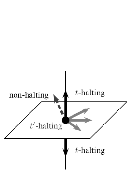
Figure 1: mutually orthogonal halting spaces.

At first, it seems that the halting conditions given above are far too restrictive. Don’t we loose a lot by dismissing every input which does not satisfy those conditions perfectly, but, say, only approximately up to some small ${\varepsilon}$? To see that it is not that bad, note that

• most (if not all) of the well-known quantum algorithms, like the quantum Fourier transform or Shor’s algorithm, have classically controlled halting. That is, the halting time is known in advance, and can be controlled by a classical subprogram.

• we show elsewehere [12] (cf. Theorem III.15) that every input that is almost halting can be modified by adding at most a constant number of qubits to halt perfectly, i.e. to satisfy the aforementioned halting conditions. This can be interpreted as some kind of “stability result”, showing that the halting conditions are not “unphysical”, but have some kind of built-in error tolerance that was not expected from the beginning.

Moreover, this definition of halting is very useful. Given two QTMs $M_{1}$ and $M_{2}$, it enables us to construct a QTM $M$ which carries out the computations of $M_{1}$, followed by the computations of $M_{2}$, just by redirecting the final state $|q_{f}\rangle$ of $M_{1}$ to the starting state $|q_{0}\rangle$ of $M_{2}$ (see [3, Dovetailing Lemma 4.2.6]). In addition, it follows from this definition that QTMs are quantum operations, which is a very useful and plausible property.

Even more important, at each single time step, an outside observer can make a measurement of the control state, described by the operators $|q_{f}\rangle\langle q_{f}|$ and $\mathbf{1}-|q_{f}\rangle\langle q_{f}|$ (thus observing the halting time), without spoiling the computation, as long as the input $|\psi\rangle$ is halting. As soon as halting is detected, the observer can extract the output quantum state from the output track (tape) and use it for further quantum information processing. This is true even if the halting time is very large, which typically happens in the study of Kolmogorov complexity. Consequently, our definition of halting has the useful property that if an outside observer is given some unknown quantum state $|\psi\rangle$ which is halting, then the observer can find out with certainty by measurement.

Finally, if we instead introduced some probabilistic notion of halting (say, we demanded that we observe halting of the QTM $M$ at some time $t$ with some large probability $p<1$), then it would not be so clear how to define quantum Kolmogorov complexity correctly. Namely if the halting probability is much less than one, it seems necessary to introduce some kind of “penalty term” into the definition of quantum Kolmogorov complexity: there should be some trade-off between program length and halting accuracy, and it is not so clear what the correct trade-off should be. For example, what is the complexity of a qubit string that has a program of length 100 which halts with probability $0.8$, and another program of length 120 which halts with probability $0.9$? The definition of halting that we use in this paper avoids such questions.

I-B Different Notions of Universality for QTMs

Bernstein and Vazirani [3] have shown that there exists a universal QTM (UQTM) $\mathcal{U}$. It is important to understand what exactly they mean by “universal”. According to [3, Thm. 7.0.2], this UQTM $\mathcal{U}$ has the property that for every QTM $M$ there is some classical bit string $s_{M}\in\{0,1\}^{*}$ (containing a description of the QTM $M$) such that

$$\left\|\mathcal{U}(s_{M},T,\delta,|\psi\rangle)-\mathcal{R}\left(M_{\mathbf{O}}^{T}(|\psi\rangle)\right)\right\|_{\rm Tr}<\delta$$ (1)

for every input $|\psi\rangle$, accuracy $\delta>0$ and number of time steps $T\in{\mathbb{N}}$. Here, $\|\cdot\|_{\rm Tr}$ is the trace distance, and $\mathcal{R}\left(M_{\mathbf{O}}^{T}(|\psi\rangle)\right)$ is the content of the output tape $\mathbf{O}$ of $M$ after $T$ steps of computation (the notation will be defined exactly in Subsection II-B).

This means that the UQTM $\mathcal{U}$ simulates every other QTM $M$ within any desired accuracy and outputs an approximation of the output track content of $M$ and halts, as long as the number of time steps $T$ is given as input in advance.

Since the purpose of Bernstein and Vazirani’s work was to study the computational complexity of QTMs, it was a reasonable assumption that the halting time $T$ is known in advance (and not too large) and can be specified as additional input. The most important point for them was not to have short inputs, but to prove that the simulation of $M$ by $\mathcal{U}$ is efficient, i.e. has only polynomial slowdown.

The situation is different if one is interested in studying quantum algorithmic information theory instead. It will be explained in Subsection I-C below that the universality notion (1) is not enough for proving the important invariance property of quantum Kolmogorov complexity, which says that quantum Kolmogorov complexity depends on the choice of the universal QTM only up to an additive constant.

To prove the invariance property, one needs a generalization of (1), where the requirement to have the running time $T$ as additional input is dropped. We show below in Section III that there exists a UQTM $\mathfrak{U}$ that satisfies such a generalized universality property, i.e. that simulates every other QTM until that other QTM has halted, without knowing that halting time in advance, and then halts itself.

Why is that so difficult to prove? At first, it seems that one can just program the UQTM $\mathcal{U}$ mentioned in (1) to simulate the other QTM $M$ for $T=1,2,3,\ldots$ time steps, and, after every time step, to check if the simulation of $M$ has halted or not. If it has halted, then $\mathcal{U}$ halts itself and prints out the output of $M$, otherwise it continues.

This approach works for classical TMs, but for QTMs, there is one problem: in general, the UQTM $\mathcal{U}$ can simulate $M$ only approximately. The reason is the same as for the circuit model, i.e. the set of basic unitary transformations that $\mathcal{U}$ can apply on its tape may be algebraically independent from that of $M$, making a perfect simulation in principle impossible. But if the simulation is only approximate, then the control state of $M$ will also be simulated only approximately, which will force $\mathcal{U}$ to halt only approximately. Thus, the restrictive halting conditions given above in Equation (6) will inevitably be violated, and the computation of $\mathcal{U}$ will be treated as invalid and be dismissed by definition.

This is a severe problem that cannot be circumvented easily. Many ideas for simple solutions must fail, for example the idea to let $\mathcal{U}$ compute an upper bound on the halting time $T$ of all inputs for $M$ of some length $n$ and just to proceed for $T$ time steps: upper bounds on halting times are not computable. Another idea is that the computation of $\mathcal{U}$ should somehow consist of a classical part that controls the computation and a quantum part that does the unitary transformations on the data. But this idea is difficult to formalize. Even for classical TMs, there is no general way to split the computation into “program” and “data” except for special cases, and for QTMs, by definition, global unitary time evolution can entangle every part of a QTM with every other part.

Our proof idea rests instead on the observation that every input for a QTM which is halting can be decomposed into a classical and a quantum part, which is related to the mutual orthogonality of the halting spaces. See Subsection I-E for details.

I-C Q-Kolmogorov Complexity and its Supposed Invariance

The classical Kolmogorov complexity $C_{U}(s)$ of a finite bit string $s\in\{0,1\}^{*}$ is defined as the minimal length of any computer program $p$ that, given as input into a TM $M$, outputs the string and makes $M$ halt:

$$C_{M}(s):=\min\left\{\ell(p)\,\,|\,\,M(p)=s\right\}.$$

For this quantity, running times are not important; all that matters is the input length. There is a crucial result that is the basis for the whole theory of Kolmogorov complexity (see [13]). Basically, it states that the choice of the computer $M$ is not important as long as $M$ is universal; choosing a different universal computer will alter the complexity only up to some additive constant. More specifically, there exists a universal computer $U$ such that for every computer $M$ there is a constant $c_{M}\in{\mathbb{N}}$ such that

$$C_{U}(s)\leq C_{M}(s)+c_{M}\qquad\mbox{for every }s\in\{0,1\}^{*}.$$ (2)

This so-called “invariance property” follows easily from the existence of a universal computer $U$ in the following sense: There exists a computer $U$ such that for every computer $M$ and every input $s\in\{0,1\}^{*}$ there is an input $\tilde{s}\in\{0,1\}^{*}$ such that $U(\tilde{s})=M(s)$ and $\ell(\tilde{s})\leq\ell(s)+c_{M}$, where $c_{M}\in{\mathbb{N}}$ is a constant depending only on $M$. In short, there is a computer $U$ that produces every output that is produced by any other computer, while the length of the corresponding input blows up only by a constant summand. One can think of the bit string $\tilde{s}$ as consisting of the original bit string $s$ and of a description of the computer $M$ (of length $c_{M}$).

The quantum generalization of Kolmogorov complexity that we consider in this paper has been first defined by Berthiaume, van Dam and Laplante [14]. Basically, they define the quantum Kolmogorov complexity $QC$ of a string of qubits $|\psi\rangle$ as the length of the shortest string of qubits that, when given as input to a QTM $M$, makes $M$ output $|\psi\rangle$ and halt. (We give a formal definition of a “qubit string” in Subsection II-A and of quantum Kolmogorov complexity $QC$ in Subsection II-C).

In [14], it is claimed that quantum Kolmogorov complexity $QC$ is invariant up to an additive constant similar to (2). It is stated there that the existence of a universal QTM $\mathcal{U}$ in the sense of Bernstein and Vazirani (see Equation (1)) makes it possible to mimic the classical proof and to conclude that the UQTM $\mathcal{U}$ outputs all that every other QTM outputs, implying invariance of quantum Kolmogorov complexity.

But this conclusion cannot be drawn so easily, because (1) demands that the halting time $T$ is specified as additional input, which can enlarge the input length dramatically, if $T$ is very large (which typically happens in the study of Kolmogorov complexity).

As explained above in Subsection I-B, it is not so easy to get rid of the halting time. The main reason is that the UQTM $\mathcal{U}$ can simulate other QTMs only approximately. Thus, it will also simulate the control state and the signaling of halting only approximately, and cannot just “halt whenever the simulation has halted”, because then, it will violate the restrictive halting conditions given in Equation (6). As we have chosen this definition of halting for good reasons (cf. the discussion at the beginning of Subsection I-A above), we do not want to drop it.

Instead of (1), a stronger notion of universality is needed, namely a “strongly universal” QTM $\mathfrak{U}$ that, as explained above in Subsection I-B, simulates every other QTM $M$ until the other QTM has halted and then halts itself with probability one, as required by the halting conditions given in Subsection I-A. Then, the classical proof outlined above can be carried over to the quantum situation. In this paper, we prove that such a QTM $\mathfrak{U}$ really exists (Theorem I.1), and as a corollary, the invariance property for quantum Kolmogorov complexity follows (Theorem I.2).

I-D Main Theorems

One main result of this paper is the existence of a “strongly universal” QTM that simulates every other QTM until the other QTM has halted and then halts itself. Note that the halting state is attained by $\mathfrak{U}$ exactly (with probability one) in accordance with the strict halting conditions stated in Equation (6). The exact definition of “qubit strings” and the output $M(\sigma)$ of $M$ on input $\sigma$ is given below in Section II.

Theorem I.1 (Strongly Universal Q-Turing Machine)

There is a fixed-length quantum Turing machine $\mathfrak{U}$ such that for every QTM $M$ and every qubit string $\sigma$ for which $M(\sigma)$ is defined, there is a qubit string $\sigma_{M}$ such that

$$\left\|\mathfrak{U}\,(\sigma_{M},\delta)-M(\sigma)\right\|_{\rm Tr}<\delta$$

for every $\delta\in\mathbb{Q}^{+}$, where the length of $\sigma_{M}$ is bounded by $\ell(\sigma_{M})\leq\ell(\sigma)+c_{M}$, and $c_{M}\in{\mathbb{N}}$ is a constant depending only on $M$.

Note that $\sigma_{M}$ does not depend on $\delta$. We conclude from this theorem and a two-parameter generalization given in Proposition III.14 that quantum Kolmogorov complexity as defined in [14] is indeed invariant, i.e. depends on the choice of the strongly universal QTM only up to some constant:

Theorem I.2 (Invariance of Q-Kolmogorov Complexity)

There is a fixed-length quantum Turing machine $\mathfrak{U}$ such that for every QTM $M$ there is a constant $c_{M}\in{\mathbb{N}}$ such that

$$QC_{\mathfrak{U}}(\rho)\leq QC_{M}(\rho)+c_{M}\qquad\mbox{for every qubit string }\rho.$$

Moreover, for every QTM $M$ and every $\delta,\Delta\in\mathbb{Q}^{+}$ with $\delta<\Delta$, there is a constant $c_{M,\delta,\Delta}\in{\mathbb{N}}$ such that

$$QC^{\Delta}_{\mathfrak{U}}(\rho)\leq QC^{\delta}_{M}(\rho)+c_{M,\delta,\Delta}\qquad\mbox{for every qubit string }\rho.$$

All the proofs are given in Section III, while the ideas of the proofs are outlined in the next subsection.

I-E Ideas of Proof

The proof of Theorem I.1 relies on the observation about the mutual orthogonality of the halting spaces, as explained in Subsection I-A. Fix some QTM $M$, and denote the set of vectors $|\psi\rangle\in\left({\mathbb{C}}^{2}\right)^{\otimes n}$ which cause $M$ to halt at time $t$ by ${\cal H}_{M}^{(n)}(t)$. If $|\varphi\rangle\in\left({\mathbb{C}}^{2}\right)^{\otimes n}$ is any halting input for $M$, then we can decompose $|\varphi\rangle$ in some sense into a classical and a quantum part. Namely, the information contained in $|\varphi\rangle$ can be split into a

• classical part: The vector $|\varphi\rangle$ is an element of which of the subspaces ${\cal H}_{M}^{(n)}(t)$?

• quantum part: Given the halting time $\tau$ of $|\varphi\rangle$, then where in the corresponding subspace ${\cal H}_{M}^{(n)}(\tau)$ is $|\varphi\rangle$ situated?

Our goal is to find a QTM $\mathfrak{U}$ and an encoding $|\tilde{\varphi}\rangle\in\left({\mathbb{C}}^{2}\right)^{\otimes(n+1)}$ of $|\varphi\rangle$ which is only one qubit longer and which makes the (cleverly programmed) QTM $\mathfrak{U}$ output a good approximation of $M(|\varphi\rangle)$. First, we extract the quantum part out of $|\varphi\rangle$. While $\dim\left({\mathbb{C}}^{2}\right)^{\otimes n}=2^{n}$, the halting space ${\cal H}_{M}^{(n)}(\tau)$ that contains $|\varphi\rangle$ is only a subspace and might have much smaller dimension $d<2^{n}$. This means that we need less than $n$ qubits to describe the state $|\varphi\rangle$; indeed, $\lceil\log_{2}d\rceil$ qubits are sufficient. In other words, there is some kind of “standard compression map” $\mathcal{C}$ that maps every vector $|\psi\rangle\in{\cal H}_{M}^{(n)}(\tau)$ into the $\lceil\log_{2}d\rceil$-qubit-space $\left({\mathbb{C}}^{2}\right)^{\otimes\lceil\log_{2}d\rceil}$. Thus, the qubit string ${\mathcal{C}}|\varphi\rangle$ of length $\lceil\log_{2}d\rceil\leq n$ can be considered as the “quantum part” of $|\varphi\rangle$.

So how can the classical part of $|\varphi\rangle$ be encoded into a short classical binary string? Our task is to specify what halting space ${\cal H}_{M}^{(n)}(\tau)$ corresponds to $|\varphi\rangle$. Unfortunately, it is not possible to encode the halting time $\tau$ directly, since $\tau$ might be huge and may not have a short description. Instead, we can encode the halting number. Define the halting time sequence $\{t_{i}\}_{i=1}^{N}$ as the set of all integers $t\in{\mathbb{N}}$ such that $\dim{\cal H}_{M}^{(n)}(t)\geq 1$, ordered such that $t_{i}<t_{i+1}$ for every $i$, that is, the set of all halting times that can occur on inputs of length $n$. Thus, there must be some $i\in{\mathbb{N}}$ such that $\tau=t_{i}$, and $i$ can be called the halting number of $|\varphi\rangle$. Now, we assign code words $c_{i}$ to the halting numbers $i$, that is, we construct a prefix code $\{c_{i}\}_{i=1}^{N}\subset\{0,1\}^{*}$. We want the code words to be short; we claim that we can always choose the lengths as

$$\ell(c_{i})=n+1-\lceil\log_{2}\dim{\cal H}_{M}^{(n)}(t_{i})\rceil\,\,.$$

This can be verified by checking the Kraft inequality:

$$\sum_{i=1}^{N}2^{-\ell(c_{i})} = 2^{-n}\sum_{i=1}^{N}2^{\lceil\log_{2}\dim{\cal H}_{M}^{(n)}(t_{i})\rceil-1}$$

$$\leq 2^{-n}\sum_{i=1}^{n}\dim{\cal H}_{M}^{(n)}(t_{i})\leq 2^{-n}\dim\left({\mathbb{C}}^{2}\right)^{\otimes n}$$

$$\leq 1,$$

since the halting spaces are mutually orthogonal.

Putting classical and quantum part of $|\varphi\rangle$ together, we get

$$|\tilde{\varphi}\rangle:=c_{i}\otimes{\mathcal{C}}|\varphi\rangle\,\,,$$

where $i$ is the halting number of $|\varphi\rangle$. Thus, the length of $|\tilde{\varphi}\rangle$ is exactly $n+1$.

Let $s_{M}$ be a self-delimiting description of the QTM $M$. The idea is to construct a QTM $\mathfrak{U}$ that, on input $s_{M}\otimes|\tilde{\varphi}\rangle$, proceeds as follows:

• By classical simulation of $M$, it computes descriptions of the halting spaces ${\cal H}_{M}^{(n)}(1),{\cal H}_{M}^{(n)}(2),{\cal H}_{M}^{(n)}(3),\ldots$ and the corresponding code words $c_{1},c_{2},c_{3},\ldots$ one after the other, until at step $\tau$, it finds the code word $c_{i}$ that equals the code word in the input.

• Afterwards, it applies a (quantum) decompression map to approximately reconstruct $|\varphi\rangle$ from ${\mathcal{C}}|\varphi\rangle$.

• Finally, it simulates (quantum) for $\tau$ time steps the time evolution of $M$ on input $|\varphi\rangle$ and then halts, whatever happens with the simulation.

Such a QTM $\mathfrak{U}$ will have the strong universality property as stated in Theorem I.1. Unfortunately, there are many difficulties that have to be overcome by the proof in Section III:

• Also classically, QTMs can only be simulated approximately. Thus, it is for example impossible for $\mathfrak{U}$ to decide by classical simulation whether the QTM $M$ halts on some input $|\psi\rangle$ perfectly or only approximately at some time $t$. Thus, we have to define certain $\delta$-approximate halting spaces ${\cal H}_{M}^{(n,\delta)}(t)$ and prove a lot of lemmas with nasty inequalities.

• Since our approach includes mixed qubit strings, we have to consider mixed inputs and outputs as well.

• The aforementioned prefix code must have the property that one code word can be constructed after the other (since the sequence of all halting times is not computable), see Lemma III.12.

We show that all these difficulties (and some more) can be overcome, and the idea outlined above can be converted to a formal proof of Theorem I.1 and the second part of Theorem I.2 which we give in full detail in Section III.

For the first part of Theorem I.2, concerning the complexity notion $QC$, a more general result is needed which is stated in Proposition III.14, since this complexity notion needs an additional parameter as input. For this proposition, the proof idea outlined above needs to be modified. The idea for the modified proof of that proposition is to make the QTM $\mathfrak{U}$ determine the halting number of the input (and thus the halting time) directly by projective measurement in the basis of (approximations of) the halting spaces. We will not prove Proposition III.14 in full detail, but only sketch the proof there, since the technical details are similar to that of the proof of Theorem I.1.

II Mathematical Framework and Formalism

Here, we introduce the formalism that is used in Section III to describe qubit strings, quantum Turing machines, and quantum Kolmogorov complexity. We denote the density operators on a Hilbert space ${\cal H}$ by $\mathcal{T}_{1}^{+}({\cal H})$ (i.e. the positive trace-class operators with trace $1$). The natural numbers will be denoted ${\mathbb{N}}=\{1,2,3,\ldots,\}$, and we use the symbols ${\mathbb{N}}_{0}:={\mathbb{N}}\cup\{0\}$ and ${\mathbb{R}}_{0}^{+}:=\{x\in{\mathbb{R}}\,\,|\,\,x\geq 0\}$ as well as $\delta_{t^{\prime}t}$, which shall be $1$ if $t^{\prime}=t$ and $0$ otherwise.

II-A Indeterminate-Length Qubit Strings

The quantum analogue of a bit string, a so-called qubit string, is a superposition of several classical bit strings. To be as general as possible, we would like to allow also superpositions of strings of different lengths like

$$|\varphi\rangle:=\frac{1}{\sqrt{2}}\left(|00\rangle+|11011\rangle\right).$$ (3)

Such quantum states are called indeterminate-length qubit strings. They have been studied by Schumacher and Westmoreland [15], as well as by Boström and Felbinger [16] in the context of lossless quantum data compression.

Let ${\cal H}_{n}:=\left({\mathbb{C}}^{\{0,1\}}\right)^{\otimes n}$ be the Hilbert space of $n$ qubits ($n\in{\mathbb{N}}_{0}$). We write ${\mathbb{C}}^{\{0,1\}}$ for ${\mathbb{C}}^{2}$ to indicate that we fix two orthonormal computational basis vectors $|0\rangle$ and $|1\rangle$. The Hilbert space ${\cal H}_{\{0,1\}^{*}}$ which contains indeterminate-length qubit strings like $|\varphi\rangle$ can be formally defined as the direct sum

$${\cal H}_{{\{0,1\}^{*}}}:=\bigoplus_{k=0}^{\infty}{\cal H}_{k}.$$

The classical finite binary strings $\{0,1\}^{*}$ are identified with the computational basis vectors in ${\cal H}_{\{0,1\}^{*}}$, i.e. ${\cal H}_{{\{0,1\}^{*}}}\simeq\ell^{2}(\{\lambda,0,1,00,01,\ldots\})$, where $\lambda$ denotes the empty string. We also use the notation ${\cal H}_{\leq n}:=\bigoplus_{k=0}^{n}{\cal H}_{k}$ and treat it as a subspace of ${\cal H}_{\{0,1\}^{*}}$.

To be as general as possible, we do not only allow superpositions of strings of different lengths, but also mixtures, i.e. our qubit strings are arbitrary density operators on ${\cal H}_{\{0,1\}^{*}}$. It will become clear in the next sections that QTMs naturally produce mixed qubit strings as outputs. Moreover, it will be a useful feature that the result of applying the partial trace to segments of qubit strings will itself be a qubit string.

Definition II.1 (Qubit Strings and their Length)

An (indeterminate-length) qubit string $\sigma$ is a density operator on ${\cal H}_{\{0,1\}^{*}}$. Normalized vectors $|\psi\rangle\in{\cal H}_{\{0,1\}^{*}}$ will also be called qubit strings, identifying them with the corresponding density operator $|\psi\rangle\langle\psi|$. The base length (or just length) of a qubit string $\sigma\in\mathcal{T}_{1}^{+}({\cal H}_{\{0,1\}^{*}})$ is defined as

$$\ell(\sigma):=\max\{\ell(s)\,\,|\,\,\langle s|\sigma|s\rangle>0,\,\,s\in{\{0,1\}^{*}}\}$$

or as $\ell(\sigma)=\infty$ if the maximum does not exist.

For example, the density operator $|\varphi\rangle\langle\varphi|$ with $|\varphi\rangle$ as defined in Equation (3) is a (pure) qubit string of length $\ell(|\varphi\rangle\langle\varphi|)=5$. This corresponds to the fact that this state $|\varphi\rangle$ needs at least $5$ cells on a QTM’s tape to be stored perfectly (compare Subsection II-B). An alternative approach would be to consider the expectation value $\bar{\ell}$ of the length instead, which has been proposed by Rogers and Vedral [17], see also the discussion in Section IV.

In contrast to classical bit strings, there are uncountably many qubit strings that cannot be perfectly distinguished by means of any quantum measurement. A good measure for the difference between two qubit strings $\sigma$ and $\rho$ is the trace distance (cf. [18])

$$\|\rho-\sigma\|_{\rm Tr}:=\frac{1}{2}{\rm Tr}\left|\rho-\sigma\right|=\frac{1}{2}\sum_{i}|\lambda_{i}|,$$ (4)

where the $\lambda_{i}$ are the eigenvalues of the trace-class operator $\rho-\sigma$. Its operational interpretation is that it gives the maximum probability of correctly distinguishing between $\rho$ and $\sigma$ by means of any single quantum measurement.

II-B Mathematical Description of Quantum Turing Machines

Bernstein and Vazirani ([3], Def. 3.2.2) define a quantum Turing machine $M$ as a triplet $(\Sigma,Q,\delta)$, where $\Sigma$ is a finite alphabet with an identified blank symbol $\#$, and $Q$ is a finite set of states with an identified initial state $q_{0}$ and final state $q_{f}\neq q_{0}$. The function $\delta:Q\times\Sigma\to\tilde{\mathbb{C}}^{\Sigma\times Q\times\{L,R\}}$ is called the quantum transition function. The symbol $\tilde{\mathbb{C}}$ denotes the set of complex numbers $\alpha\in{\mathbb{C}}$ such that there is a deterministic algorithm that computes the real and imaginary parts of $\alpha$ to within $2^{-n}$ in time polynomial in $n$.

One can think of a QTM as consisting of a two-way infinite tape $\mathbf{T}$ of cells indexed by ${\mathbb{Z}}$, a control $\mathbf{C}$, and a single “read/write” head $\mathbf{H}$ that moves along the tape. A QTM evolves in discrete, integer time steps, where at every step, only a finite number of tape cells is non-blank. For every QTM, there is a corresponding Hilbert space ${\cal H}_{QTM}={\cal H}_{\mathbf{C}}\otimes{\cal H}_{\mathbf{T}}\otimes{\cal H}_{\mathbf{H}}$, where ${\cal H}_{\mathbf{C}}={\mathbb{C}}^{Q}$ is a finite-dimensional Hilbert space spanned by the (orthonormal) control states $q\in Q$, while ${\cal H}_{\mathbf{T}}=\ell^{2}(T)$ and ${\cal H}_{\mathbf{H}}=\ell^{2}(\mathbb{Z})$ are separable Hilbert spaces describing the contents of the tape and the position of the head, where

$$T=\left\{(x_{i})_{i\in{\mathbb{Z}}}\in\Sigma^{\mathbb{Z}}\,\,|\,\,x_{i}\neq\#\mbox{ for finitely many }i\in{\mathbb{Z}}\right\}$$ (5)

denotes the set of classical tape configurations with finitely many non-blank symbols.

For our purpose, it is useful to consider a special class of QTMs with the property that their tape $\mathbf{T}$ consists of two different tracks (cf. [3, Def. 3.5.5]), an input track $\mathbf{I}$ and an output track $\mathbf{O}$. This can be achieved by having an alphabet which is a Cartesian product of two alphabets, in our case $\Sigma=\{0,1,\#\}\times\{0,1,\#\}$. Then, the tape Hilbert space ${\cal H}_{\mathbf{T}}$ can be written as ${\cal H}_{\mathbf{T}}={\cal H}_{\mathbf{I}}\otimes{\cal H}_{\mathbf{O}}$.

The transition function $\delta$ generates a linear operator $U_{M}$ on ${\cal H}_{QTM}$ describing the time evolution of the QTM $M$. If $\delta$ is chosen in accordance with certain conditions, then $U_{M}$ will be unitary (and thus compatible with quantum theory), see Ozawa and Nishimura [5]. We identify $\sigma\in\mathcal{T}_{1}^{+}({\cal H}_{\{0,1\}^{*}})$ with the initial state of $M$ on input $\sigma$, which is according to the definition in [3] a state on ${\cal H}_{QTM}$ where $\sigma$ is written on the input track over the cell interval $[0,\ell(\sigma)-1]$, the empty state $\#$ is written on the remaining cells of the input track and on the whole output track, the control is in the initial state $q_{0}$ and the head is in position $0$. By linearity, this e.g. means that the vector $|\psi\rangle=\frac{1}{\sqrt{2}}\left(|0\rangle+|11\rangle\right)$ is identified with the vector $\frac{1}{\sqrt{2}}\left(|0\#\rangle+|11\rangle\right)$ on input track cells number $0$ and $1$.

The global state $M^{t}(\sigma)\in\mathcal{T}_{1}^{+}({\cal H}_{QTM})$ of $M$ on input $\sigma$ at time $t\in{\mathbb{N}}_{0}$ is given by $M^{t}(\sigma)=\left(U_{M}\right)^{t}\sigma\left(U_{M}^{*}\right)^{t}$. The state of the control at time $t$ is thus given by partial trace over all the other parts of the machine, that is $M_{\mathbf{C}}^{t}(\sigma):={\rm Tr}_{\mathbf{T,H}}\left(M^{t}(\sigma)\right)$ (similarly for the other parts of the QTM). In accordance with [3, Def. 3.5.1], we say that the QTM $M$ halts at time $t\in{\mathbb{N}}$ on input $\sigma\in\mathcal{T}_{1}^{+}({\cal H}_{\{0,1\}^{*}})$, if and only if

$$\langle q_{f}|M_{\rm\bf C}^{t}(\sigma)|q_{f}\rangle=1\mbox{ and }\langle q_{f}|M_{\rm\bf C}^{t^{\prime}}(\sigma)|q_{f}\rangle=0\quad\forall t^{\prime}<t,$$ (6)

where $q_{f}\in Q$ is the final state of the control (specified in the definition of $M$) signalling the halting of the computation. See Subsection I-A for a detailed discussion of these halting conditions (6).

In this paper, when we talk about a QTM, we do not mean the machine model itself, but rather refer to the corresponding partial function on the qubit strings which is computed by the QTM. Note that this point of view is different from e.g. that of Ozawa [9] who describes a QTM as a map from $\Sigma^{*}$ to the set of probability distributions on $\Sigma^{*}$.

We still have to define what is meant by the output of a QTM $M$, once it has halted at some time $t$ on some input qubit string $\sigma$. We could take the state of the output tape $M_{\mathbf{O}}^{t}(\sigma)$ to be the output, but this is not a qubit string, but instead a density operator on the Hilbert space ${\cal H}_{\mathbf{O}}$. Hence, we define a quantum operation $\mathcal{R}$ which maps the density operators on ${\cal H}_{\mathbf{O}}$ to density operators on ${\cal H}_{\{0,1\}^{*}}$, i.e. to the qubit strings. The operation $\mathcal{R}$ “reads” the output from the tape.

Definition II.2 (Reading Operation)

A quantum operation $\mathcal{R}:\mathcal{T}({\cal H}_{\mathbf{O}})\to\mathcal{T}({\cal H}_{\{0,1\}^{*}})$ is called a reading operation, if for every finite set of classical strings $\{s_{i}\}_{i=1}^{N}\subset{\{0,1\}^{*}}$, it holds that

$$\mathcal{R}\left(\mathbb{P}\left(\sum_{i=1}^{N}\alpha_{i}\left|\begin{array}[]{ccccccc}\ldots&\#&\#&s_{i}&\#&\#&\ldots\\ &\mbox{\tiny-2}&\mbox{\tiny-1}&\mbox{\tiny 0}&\mbox{\tiny$\ell(s_{i})$}&\mbox{\tiny$\ell(s_{i})+1$}&\end{array}\right\rangle\right)\right)$$

$$=\mathbb{P}\left(\sum_{i=1}^{N}\alpha_{i}|s_{i}\rangle\right)$$

where $\mathbb{P}(|\varphi\rangle):=|\varphi\rangle\langle\varphi|$ denotes the projector onto $|\varphi\rangle$.

The condition specified above does not determine $\mathcal{R}$ uniquely; there are many different reading operations. For the remainder of this paper, we fix the reading operation $\mathcal{R}$ which is specified in the following example.

Example II.3

Let $T$ denote the classical output track configurations as defined in Equation (5), with $\Sigma=\{0,1,\#\}$. Then, for every $t\in T$, let $R(t)$ be the classical string that consists of the bits of $T$ from cell number zero to the last non-blank cell, i.e.

$$R : T\to{\{0,1\}^{*}}$$

$$\left(\begin{array}[]{ccccccc}\ldots&?&?&s&\#&?&\ldots\\ &\mbox{\tiny-2}&\mbox{\tiny-1}&\mbox{\tiny 0}&\mbox{\tiny$\ell(s)$}&\mbox{\tiny$\ell(s)+1$}&\end{array}\right)\mapsto s.$$

For every $s\in{\{0,1\}^{*}}$, there is a countably-infinite number of $t\in T$ such that $R(t)=s$. Thus, to every $t\in T$, we can assign a natural number $n(t)$ which is the number of $t$ in some enumeration of the set $\{t^{\prime}\in T\,\,|\,\,R(t^{\prime})=R(t)\}$; we only demand that $n(t)=1$ if $t=\left(\begin{array}[]{ccccccc}\ldots&\#&\#&s&\#&\#&\ldots\\ &\mbox{\tiny-2}&\mbox{\tiny-1}&\mbox{\tiny 0}&\mbox{\tiny$\ell(s)$}&\mbox{\tiny$\ell(s)+1$}&\end{array}\right)$. Hence, if (as usual) $\ell^{2}\equiv\ell^{2}({\mathbb{N}})$ denotes the Hilbert space of square-summable sequences, then the map $U$, defined by linear extension of

$$U:{\cal H}_{\mathbf{O}} \to {\cal H}_{\{0,1\}^{*}}\otimes\ell^{2}$$

$$|t\rangle \mapsto |R(t)\rangle\otimes|n(t)\rangle,$$

is unitary. Then, the quantum operation

$$\mathcal{R}:\mathcal{T}({\cal H}_{\mathbf{O}}) \to \mathcal{T}({\cal H}_{\{0,1\}^{*}})$$

$$\rho \mapsto {\rm Tr}_{\ell^{2}}\left(U\rho U^{*}\right)$$

is a reading operation.

We are now ready to define QTMs as partial maps on the qubit strings.

Definition II.4 (Quantum Turing Machine (QTM))

A partial map $M:\mathcal{T}_{1}^{+}({\cal H}_{\{0,1\}^{*}})\to\mathcal{T}_{1}^{+}({\cal H}_{\{0,1\}^{*}})$ will be called a QTM, if there is a Bernstein-Vazirani two-track QTM $M^{\prime}=(\Sigma,Q,\delta)$ (see [3], Def. 3.5.5) with the following properties:

• $\Sigma=\{0,1,\#\}\times\{0,1,\#\}$,

• the corresponding time evolution operator $U_{M^{\prime}}$ is unitary,

• if $M^{\prime}$ halts on input $\sigma$ at some time $t\in{\mathbb{N}}$, then $M(\sigma)=\mathcal{R}\left({M^{\prime}}_{\mathbf{O}}^{t}(\sigma)\right)$, where $\mathcal{R}$ is the reading operation specified in Example II.3 above. Otherwise, $M(\sigma)$ is undefined.

A fixed-length QTM is the restriction of a QTM to the domain $\bigcup_{n\in{\mathbb{N}}_{0}}\mathcal{T}_{1}^{+}({\cal H}_{n})$ of length eigenstates.

The definition of halting, given by Equation (6), is very important, as explained in Subsection I-A. On the other hand, changing certain details in a QTM’s definition, like the way to read the output or allowing a QTM’s head to stay at its position instead of turning left or right, should not change the results in this paper.

II-C Quantum Kolmogorov Complexity

Quantum Kolmogorov complexity has first been defined by Berthiaume, van Dam, and Laplante [14]. They define the complexity $QC(\rho)$ of a qubit string $\rho$ as the length of the shortest qubit string that, given as input into a QTM $M$, makes $M$ output $\rho$ and halt. Since there are uncountably many qubit strings, but a QTM can only apply a countable number of transformations (analogously to the circuit model), it is necessary to introduce a certain error tolerance $\delta>0$.

This can be done in essentially two ways: First, one can just fix some tolerance $\delta$. Second, one can demand that the QTM outputs the qubit string $\rho$ as accurately as one wants, by supplying the machine with a second parameter as input that represents the desired accuracy. This is analogous to a classical computer program that computes the number $\pi=3.14\ldots$: A second parameter $k\in{\mathbb{N}}$ can make the program output $\pi$ to $k$ digits of accuracy, for example. We consider both approaches and follow the lines of [14] except for two simple modifications: we use the trace distance rather than the fidelity, and we also allow indeterminate-length and mixed input and output qubit strings.

Definition II.5 (Quantum Kolmogorov Complexity)

Let $M$ be a QTM and $\rho\in\mathcal{T}_{1}^{+}({\cal H}_{\{0,1\}^{*}})$ a qubit string. For every $\delta>0$, we define the finite-error quantum Kolmogorov complexity $QC_{M}^{\delta}(\rho)$ as the minimal length of any qubit string $\sigma\in\mathcal{T}_{1}^{+}({\cal H}_{\{0,1\}^{*}})$ such that the corresponding output $M(\sigma)$ has trace distance from $\rho$ smaller than $\delta$,

$$QC_{M}^{\delta}(\rho):=\min\left\{\ell(\sigma)\,\,|\,\,\|\rho-M(\sigma)\|_{\rm Tr}<\delta\right\}.$$

Similarly, we define the approximation-scheme quantum Kolmogorov complexity $QC_{M}(\rho)$ as the minimal length of any qubit string $\sigma\in\mathcal{T}_{1}^{+}({\cal H}_{\{0,1\}^{*}})$ such that when given $M$ as input together with any integer $k$, the output $M(\sigma,k)$ has trace distance from $\rho$ smaller than $1/k$:

$$QC_{M}(\rho):=\min\left\{\ell(\sigma)\,\,\left|\|\rho-M(\sigma,k)\|_{\rm Tr}<\frac{1}{k}\forall k\in{\mathbb{N}}\right.\right\}.$$

For the definition of $QC_{M}$, we have to fix a map to encode two inputs (a qubit string and an integer) into one qubit string; this is easy, see e.g. [13] for the classical case and [19] for the quantum case. Also, using $f(k):=1/k$ as accuracy required on input $k$ is not important; any other computable and strictly decreasing function $f$ that tends to zero for $k\to\infty$ such that $f^{-1}$ is also computable will give the same result up to an additive constant.

Note that if $M$ is at least able to move input data to the output track, then it holds $QC_{M}^{\delta}(\rho)\leq\ell(\rho)+c_{M}$ with some constant $c_{M}\in{\mathbb{N}}$ (and similarly for $QC_{M}$). In [19], we have shown that for ergodic quantum information sources, emitted states $|\psi\rangle\in\left({\mathbb{C}}^{2}\right)^{\otimes n}$ have a complexity rate $\frac{1}{n}QC_{\mathcal{U}}^{\bullet}(|\psi\rangle)$ that is with asymptotic probability $1$ arbitrarily close to the von Neumann entropy rate $s$ of the source. This demonstrates that quantum Kolmogorov complexity is a useful notion, and that it is feasible to prove interesting theorems on it.

While this complexity notion $QC(\rho)$ counts the length of the shortest qubit string that makes a QTM output $\rho$ and halt, there have been different definitions for quantum algorithmic complexity by Vitányi [20] and Gács [21]. Their approaches are based on classical descriptions and universal density matrices respectively and are not considered in this paper since they do not have the invariance problem outlined in Subsection I-C.

Note also that Definition II.5 depends on the definition of the length $\ell(\sigma)$ of a qubit string $\sigma\in\mathcal{T}_{1}^{+}({\cal H}_{\{0,1\}^{*}})$; there is a different approach by Rogers and Vedral [17] that uses the expected (average) length $\bar{\ell}$ instead and results in a different notion of quantum Kolmogorov complexity. The results of this paper are applicable to that definition, too, as long as the notion of halting of the corresponding quantum computer is defined in a deterministic way as in Equation (6).

III Construction of a Strongly Universal QTM

III-A Halting Subspaces and their Orthogonality

As already explained in Subsection I-A in the introduction, restricting to pure input qubit strings $|\psi\rangle\in{\cal H}_{n}$ of some fixed length $\ell(|\psi\rangle)=n$, the vectors with equal halting time $t$ form a linear subspace of ${\cal H}_{n}$. Moreover, inputs with different halting times are mutually orthogonal, as depicted in Figure 1. We will now use the formalism for QTMs introduced in Subsection II-B to give a formal proof of these statements. We use the subscripts $\mathbf{C}$, $\mathbf{I}$, $\mathbf{O}$ and $\mathbf{H}$ to indicate to what part of the tensor product Hilbert space a vector belongs.

Definition III.1 (Halting Qubit Strings)

Let $\sigma\in\mathcal{T}_{1}^{+}({\cal H}_{\{0,1\}^{*}})$ be a qubit string and $M$ a quantum Turing machine. Then, $\sigma$ is called $t$-halting (for $M$), if $M$ halts on input $\sigma$ at time $t\in{\mathbb{N}}$. We define the halting sets and halting subspaces

$$H_{M}(t) := \{|\psi\rangle\in{\cal H}_{\{0,1\}^{*}}\,\,|\,\,|\psi\rangle\langle\psi|\mbox{ is }t\mbox{-halting for }M\},$$

$${\cal H}_{M}(t) := \{\alpha|\psi\rangle\enspace|\enspace|\psi\rangle\in H_{M}(t),\alpha\in{\mathbb{R}}\},$$

$$H_{M}^{(n)}(t) := H_{M}(t)\cap{\cal H}_{n},\qquad{\cal H}_{M}^{(n)}(t):={\cal H}_{M}(t)\cap{\cal H}_{n}.$$

Note that the only difference between $H_{M}^{(n)}(t)$ and ${\cal H}_{M}^{(n)}(t)$ is that the latter set contains non-normalized vectors. It will be shown below that ${\cal H}_{M}^{(n)}(t)$ is indeed a linear subspace.

Theorem III.2 (Halting Subspaces)

For every QTM $M$, $n\in{\mathbb{N}}_{0}$ and $t\in{\mathbb{N}}$, the sets ${\cal H}_{M}(t)$ and ${\cal H}_{M}^{(n)}(t)$ are linear subspaces of ${\cal H}_{\{0,1\}^{*}}$ resp. ${\cal H}_{n}$, and

$${\cal H}_{M}^{(n)}(t)\perp{\cal H}_{M}^{(n)}(t^{\prime})\quad\mbox{and}\quad{\cal H}_{M}(t)\perp{\cal H}_{M}(t^{\prime})\quad\mbox{if }t\neq t^{\prime}.$$

Proof. Let $|\varphi\rangle,|\psi\rangle\in H_{M}(t)$. The property that $|\varphi\rangle$ is $t$-halting is equivalent to the statement that there are states $|\Phi_{q}^{t^{\prime}}\rangle\in{\cal H}_{\mathbf{I}}\otimes{\cal H}_{\mathbf{O}}\otimes{\cal H}_{\mathbf{H}}$ and coefficients $c_{q}^{t^{\prime}}\in{\mathbb{C}}$ for every $t^{\prime}\leq t$ and $q\in Q$ such that

$$V_{M}^{t}\left(|\varphi\rangle_{\mathbf{I}}\otimes|\Psi_{0}\rangle\right) = |q_{f}\rangle_{\mathbf{C}}\otimes|\Phi_{q_{f}}^{t}\rangle\,\,,$$ (9)

$$V_{M}^{t^{\prime}}\left(|\varphi\rangle_{\mathbf{I}}\otimes|\Psi_{0}\rangle\right) = \sum_{q\neq q_{f}}c_{q}^{t^{\prime}}|q\rangle_{\mathbf{C}}\otimes|\Phi_{q}^{t^{\prime}}\rangle\quad\forall t^{\prime}<t,$$ (10)

where $V_{M}$ is the unitary time evolution operator for the QTM $M$ as a whole, and $|\Psi_{0}\rangle=|q_{0}\rangle_{\mathbf{C}}\otimes|\#\rangle_{\mathbf{O}}\otimes|0\rangle_{\mathbf{H}}$ denotes the initial state of the control, output track and head. Note that $|\Psi_{0}\rangle$ does not depend on the input qubit string (in this case $|\varphi\rangle$).

An analogous equation holds for $|\psi\rangle$, since it is also $t$-halting by assumption. Consider a normalized superposition $\alpha|\varphi\rangle+\beta|\psi\rangle\in{\cal H}_{\{0,1\}^{*}}$:

$$V_{M}^{t}\left(\right.\left(\alpha|\varphi\rangle_{\mathbf{I}}+\beta|\psi\rangle_{\mathbf{I}}\right)\otimes|\Psi_{0}\rangle\left.\right)$$

$$\qquad\qquad=\alpha V_{M}^{t}|\varphi\rangle_{\mathbf{I}}\otimes|\Psi_{0}\rangle+\beta V_{M}^{t}|\psi\rangle_{\mathbf{I}}\otimes|\Psi_{0}\rangle$$

$$\qquad\qquad=\alpha|q_{f}\rangle_{\mathbf{C}}\otimes|\Phi_{q_{f}}^{t}\rangle+\beta|q_{f}\rangle_{\mathbf{C}}\otimes|\tilde{\Phi}_{q_{f}}^{t}\rangle$$

$$\qquad\qquad=|q_{f}\rangle_{\mathbf{C}}\otimes\left(\alpha|\Phi_{q_{f}}^{t}\rangle+\beta|\tilde{\Phi}_{q_{f}}^{t}\rangle\right).$$

Thus, the superposition also satisfies condition (9), and, by a similar calculation, condition (10). It follows that $\alpha|\varphi\rangle+\beta|\psi\rangle$ must also be $t$-halting. Hence, ${\cal H}_{M}(t)$ is a linear subspace of ${\cal H}_{\{0,1\}^{*}}$. As the intersection of linear subspaces is again a linear subspace, so must be ${\cal H}_{M}^{(n)}(t)$.

Let now $|\varphi\rangle\in H_{M}(t)$ and $|\psi\rangle\in H_{M}(t^{\prime})$ such that $t<t^{\prime}$. Again by Equations (9) and (10), it holds

$$\langle\varphi|\psi\rangle = \left(\,{}_{\mathbf{I}}\langle\varphi|\otimes\langle\Psi_{0}|\right)\left(V_{M}^{t}\right)^{*}V_{M}^{t}\left(|\psi\rangle_{\mathbf{I}}\otimes|\Psi_{0}\rangle\right)$$

$$= \sum_{Q\ni q\neq q_{f}}c_{q}^{t}\underbrace{\enspace{}_{\mathbf{C}}\langle q_{f}|q\rangle_{\mathbf{C}}}_{0}\cdot\langle\Phi_{q_{f}}^{t}|\tilde{\Phi}_{q}^{t}\rangle=0\,\,.$$

It follows that ${\cal H}_{M}(t)\perp{\cal H}_{M}(t^{\prime})$, and similarly for ${\cal H}_{M}^{(n)}(\cdot)\subset{\cal H}_{M}(\cdot)$. ∎The physical interpretation of the preceding theorem is straightforward: By linearity of the time evolution, superpositions of $t$-halting strings are again $t$-halting, and strings with different halting times can be perfectly distinguished by observing their halting time.

III-B Approximate Halting Spaces

The aim of this subsection is to show that the halting spaces of a QTM can be numerically approximated by a classical algorithm. Thus, we give a step by step construction of such an algorithm, and show analytically that the approximations it computes are good enough for our purpose. The main result is given in Theorem III.4. Before we state that theorem, we fix some notation.

Definition III.3 (${\varepsilon}$-$t$-halting Property)

A qubit string $\sigma\in\mathcal{T}_{1}^{+}({\cal H}_{\{0,1\}^{*}})$ will be called ${\varepsilon}$-$t$-halting for $M$ for some $t\in{\mathbb{N}}$, ${\varepsilon}\geq 0$ and $M$ a QTM, if and only if

$$\langle q_{f}|M_{\mathbf{C}}^{t^{\prime}}(\sigma)|q_{f}\rangle\left\{\begin{array}[]{ll}\leq{\varepsilon}&\mbox{for }t^{\prime}<t\,\,,\\ \geq 1-{\varepsilon}&\mbox{for }t^{\prime}=t\,\,.\end{array}\right.$$

We denote by $S_{n}:=\left\{|\psi\rangle\in{{\cal H}_{n}}\enspace|\enspace\||\psi\rangle\|=1\right\}$ the unit sphere in ${{\cal H}_{n}}\equiv\left({\mathbb{C}}^{2}\right)^{\otimes n}$, and by $U_{\delta}(|\varphi\rangle):=\left\{|\psi\rangle\in{{\cal H}_{n}}\enspace|\enspace\||\psi\rangle-|\varphi\rangle\|<\delta\right\}$ an open ball. The ball $U_{\delta}(|\varphi\rangle)$ will be called ${\varepsilon}$-$t$-halting for $M$ if there is some $|\psi\rangle\in U_{\delta}(|\varphi\rangle)\cap S_{n}$ which is ${\varepsilon}$-$t$-halting for $M$. Moreover, we use the following symbols:

• ${\rm dist}(S,|\varphi\rangle):=\inf_{s\in S}\|\,|s\rangle-|\varphi\rangle\|$ for any subset $S\subset{{\cal H}_{n}}$ and $|\varphi\rangle\in{{\cal H}_{n}}$,

• ${{\cal H}_{n}^{\mathbb{Q}}}:=\left\{|\varphi\rangle\in{{\cal H}_{n}}\,\,|\,\,\langle e_{k}|\varphi\rangle\in\mathbb{Q}+i\mathbb{Q}\quad\forall k\right\}$, where $\{|e_{k}\rangle\}_{k=1}^{2^{n}}$ denotes the computational basis vectors of ${{\cal H}_{n}}$,

• $|\varphi^{0}\rangle:=\frac{|\varphi\rangle}{\|\,|\varphi\rangle\|}$ for every vector $|\varphi\rangle\in{{\cal H}_{n}}\setminus\{0\}$.

The set of vectors with rational coordinates, denoted ${{\cal H}_{n}^{\mathbb{Q}}}$, will in the following be used frequently as inputs or outputs of algorithms. Such vectors can be symbolically added or multiplied with rational scalars without any error. Also, given $|a\rangle,|b\rangle\in{{\cal H}_{n}^{\mathbb{Q}}}$, it is an easy task to decide unambiguously which vector has larger norm than the other (one can compare the rational numbers $\|\,|a\rangle\|^{2}$ and $\|\,|b\rangle\|^{2}$, for example).

Now we are ready to state the main theorem of this subsection:

Theorem III.4 (Computable Approximate Halting Spaces)

There is a classical algorithm that, given a classical description of a QTM $M$, integers $n\in{\mathbb{N}}_{0}$, $t\in{\mathbb{N}}$, and a rational parameter $\delta>0$, computes a description of some subspace ${\cal H}_{M}^{(n,\delta)}(t)\subset{\cal H}_{n}$ and a rational number ${\varepsilon}_{M}^{(n,\delta)}(t)>0$ with the following properties:

• Almost-Halting: If $|\psi\rangle\in H_{M}^{(n,\delta)}(t)$, then $|\psi\rangle$ is $(20\,\delta)$-$t$-halting for $M$.

• Approximation: For every $|\psi\rangle\in H_{M}^{(n)}(t)$, there is a vector $|\psi^{(\delta)}\rangle\in H_{M}^{(n,\delta)}(t)$ which satisfies $\|\,|\psi\rangle-|\psi^{(\delta)}\rangle\|<\frac{11}{2}\delta$.

• Similarity: If $\delta,\Delta\in\mathbb{Q}^{+}$ such that $\delta\leq\frac{1}{80}\,{\varepsilon}_{M}^{(n,\Delta)}(t)$, then for every $|\psi\rangle\in H_{M}^{(n,\delta)}(t)$ there is a vector $|\psi^{(\Delta)}\rangle\in H_{M}^{(n,\Delta)}(t)$ which satisfies $\|\,|\psi\rangle-|\psi^{(\Delta)}\rangle\|<\frac{11}{2}\Delta$.

• Almost-Orthogonality: If $|\psi_{t}\rangle\in H_{M}^{(n,\delta)}(t)$ and $|\psi_{t^{\prime}}\rangle\in H_{M}^{(n,\delta)}(t^{\prime})$ for $t\neq t^{\prime}$, then it holds that $|\langle\psi_{t}|\psi_{t^{\prime}}\rangle|\leq 4\sqrt{5\delta}$.

The description of this algorithm (Definition III.7) and the proof of this theorem (on page III.8) need some lemmas that show how certain computational steps can be accomplished.

Lemma III.5 (Algorithm for ${\varepsilon}$-$t$-halting-Property of Balls)

There exists a (classical) algorithm $B$ which, on input $|\varphi\rangle\in{{\cal H}_{n}^{\mathbb{Q}}}$, $\delta,{\varepsilon}\in\mathbb{Q}^{+}$, $t\in{\mathbb{N}}$ and a classical description $s_{M}\in\{0,1\}^{*}$ of a fixed-length QTM $M$, always halts and returns either $0$ or $1$ under the following constraints:

• If $U_{\delta}(|\varphi\rangle)$ is not ${\varepsilon}$-$t$-halting for $M$, then the output must be $0$.

• If $U_{\delta}(|\varphi\rangle)$ is $\frac{{\varepsilon}}{4}$-$t$-halting for $M$, then the output must be $1$.

Proof. The algorithm $B$ computes a set of vectors $\{|\varphi_{k}\rangle\}_{k=1}^{N}\subset{{\cal H}_{n}^{\mathbb{Q}}}$ such that for every vector $|\psi\rangle\in U_{\delta}(|\varphi\rangle)\cap S_{n}$ there is a $k\in\{1,\ldots,N\}$ such that $\|\,|\varphi_{k}\rangle-|\psi\rangle\|\leq\frac{3}{64}\,{\varepsilon}$, and also vice versa (i.e. ${\rm dist}\left(U_{\delta}(|\varphi\rangle)\cap S_{n},|\varphi_{k}\rangle\right)\leq\frac{3}{64}\,{\varepsilon}$ for every $k$).

For every $k\in\{1,\ldots,N\}$, the algorithm simulates the QTM $M$ on input $|\varphi_{k}\rangle$ classically for $t$ time steps and computes an approximation $a(t^{\prime})$ of the quantity $\langle q_{f}|M_{\mathbf{C}}^{t^{\prime}}(|\varphi_{k}\rangle\langle\varphi_{k}|)|q_{f}\rangle$ for every $t^{\prime}\leq t$, such that

$$\left|a(t^{\prime})-\langle q_{f}|M_{\mathbf{C}}^{t^{\prime}}(|\varphi_{k}\rangle\langle\varphi_{k}|)|q_{f}\rangle\right|<\frac{3}{32}\,{\varepsilon}\qquad\mbox{for every }t^{\prime}\leq t\,\,.$$

How can this be achieved? Since the number of time steps $t$ is finite, time evolution will be restricted to a finite subspace $\tilde{\cal H}_{\mathbf{T}}\subset{\cal H}_{\mathbf{T}}$ corresponding to a finite number of tape cells, which also restricts the state space of the head (that points on tape cells) to a finite subspace $\tilde{\cal H}_{\mathbf{H}}$. Thus, it is possible to give a matrix representation of the time evolution operator $V_{M}$ on ${\cal H}_{\mathbf{C}}\otimes\tilde{\cal H}_{\mathbf{T}}\otimes\tilde{\cal H}_{\mathbf{H}}$, and the expression given above can be numerically calculated just by matrix multiplication and subsequent numerical computation of the partial trace.

Every $|\varphi_{k}\rangle$ that satisfies $|a(t^{\prime})-\delta_{t^{\prime}t}|\leq\frac{5}{8}\,{\varepsilon}$ for every $t^{\prime}\leq t$ will be marked as “approximately halting”. If there is at least one $|\varphi_{k}\rangle$ that is approximately halting, $B$ shall halt and output $1$, otherwise it shall halt and output $0$.

To see that this algorithm works as claimed, suppose that $U_{\delta}(|\varphi\rangle)$ is not ${\varepsilon}$-$t$-halting for $M$, so for every $|\tilde{\psi}\rangle\in U_{\delta}(|\varphi\rangle)$ there is some $t^{\prime}\leq t$ such that $\left|\delta_{t^{\prime}t}-\langle q_{f}|M_{\mathbf{C}}^{t^{\prime}}(|\tilde{\psi}\rangle\langle\tilde{\psi}|)|q_{f}\rangle\right|>{\varepsilon}$. Also, for every $k\in\{1,\ldots,N\}$, there is some vector $|\psi\rangle\in U_{\delta}(|\varphi\rangle)\cap S_{n}$ with $\|\,|\varphi_{k}\rangle-|\psi\rangle\|\leq\frac{3}{64}\,{\varepsilon}$, so

$$\Delta_{k} := \left|\delta_{t^{\prime}t}-\langle q_{f}|M_{\mathbf{C}}^{t^{\prime}}(|\varphi_{k}\rangle\langle\varphi_{k}|)|q_{f}\rangle\right|$$

$$\geq \left|\delta_{t^{\prime}t}-\langle q_{f}|M_{\mathbf{C}}^{t^{\prime}}(|\psi\rangle\langle\psi|)|q_{f}\rangle\right|$$

$$- \left|\langle q_{f}|M_{\mathbf{C}}^{t^{\prime}}(|\psi\rangle\langle\psi|)|q_{f}\rangle-\langle q_{f}|M_{\mathbf{C}}^{t^{\prime}}(|\varphi_{k}^{0}\rangle\langle\varphi_{k}^{0}|)|q_{f}\rangle\right|$$

$$- \left|\langle q_{f}|M_{\mathbf{C}}^{t^{\prime}}(|\varphi_{k}\rangle\langle\varphi_{k}|)|q_{f}\rangle-\langle q_{f}|M_{\mathbf{C}}^{t^{\prime}}(|\varphi_{k}^{0}\rangle\langle\varphi_{k}^{0}|)|q_{f}\rangle\right|$$

$$> {\varepsilon}-\|\,|\psi\rangle\langle\psi|-|\varphi_{k}^{0}\rangle\langle\varphi_{k}^{0}|\|_{\rm{Tr}}-2\cdot\left|1-\|\,|\varphi_{k}\rangle\|^{2}\right|$$

$$\geq {\varepsilon}-\|\,|\psi\rangle-|\varphi_{k}^{0}\rangle\|-2\left|1-\|\,|\varphi_{k}\rangle\|\right|(1+\|\,|\varphi_{k}\rangle\|)$$

$$\geq {\varepsilon}-\frac{3}{64}\,{\varepsilon}-\|\,|\varphi_{k}\rangle-|\varphi_{k}^{0}\rangle\|-4\cdot\frac{3}{64}\,{\varepsilon}\geq\frac{23}{32}{\varepsilon}\,\,,$$

where we have used Lemma .3 and Lemma .5. Thus, for every $k$ it holds

$$\left|a(t^{\prime})-\delta_{t^{\prime}t}\right| \geq \Delta_{k}-\left|\langle q_{f}|M_{\mathbf{C}}^{t^{\prime}}(|\varphi_{k}\rangle\langle\varphi_{k}|)|q_{f}\rangle-a(t^{\prime})\right|$$

$$> \frac{23}{32}{\varepsilon}-\frac{3}{32}\,{\varepsilon}=\frac{5}{8}{\varepsilon}\,\,,$$

which makes the algorithm halt and output $0$.

On the other hand, suppose that $U_{\delta}(|\varphi\rangle)$ is $\frac{{\varepsilon}}{4}$-$t$-halting for $M$, i.e. there is some $|\psi\rangle\in U_{\delta}(|\varphi\rangle)\cap S_{n}$ which is $\frac{{\varepsilon}}{4}$-$t$-halting for $M$. By construction, there is some $k$ such that $\|\,|\varphi_{k}\rangle-|\psi\rangle\|\leq\frac{3}{64}\,{\varepsilon}$. A similar calculation as above yields $\left|\delta_{t^{\prime}t}-\langle q_{f}|M_{\mathbf{C}}^{t^{\prime}}(|\varphi_{k}\rangle\langle\varphi_{k}|)|q_{f}\rangle\right|\leq\frac{17}{32}{\varepsilon}$ for every $t^{\prime}\leq t$, so $\left|a(t^{\prime})-\delta_{t^{\prime}t}\right|\leq\frac{17}{32}{\varepsilon}+\frac{3}{32}\,{\varepsilon}=\frac{5}{8}\,{\varepsilon}$, and the algorithm outputs $1$.∎

Lemma III.6 (Algorithm $I$ for Interpolating Subspace)

There exists a (classical) algorithm $I$ which, on input $M,N\in{\mathbb{N}}$, $|\tilde{\varphi}_{1}\rangle,\ldots,|\tilde{\varphi}_{M}\rangle$, $|\varphi_{1}\rangle,\ldots,|\varphi_{N}\rangle\in{{\cal H}_{n}^{\mathbb{Q}}}$, $d\in{\mathbb{N}}$, $\mathbb{Q}^{+}\ni\Delta>\delta$ and $\mathbb{Q}^{+}\ni\tilde{\Delta}>\tilde{\delta}$, always halts and returns the description of a pair $(i,\tilde{U})$ with $i\in\{0,1\}$ and $\tilde{U}\subset{{\cal H}_{n}}$ a linear subspace, under the following constraints:

• If the output is $(1,\tilde{U})$, then $\tilde{U}\subset{{\cal H}_{n}}$ must be a subspace of dimension $\dim\tilde{U}=d$ such that ${\rm dist}(\tilde{U},|\varphi_{k}\rangle)<\Delta$ for every $k$ and ${\rm dist}(\tilde{U},|\tilde{\varphi}_{l}\rangle)>\tilde{\delta}$ for every $l$.

• If there exists a subspace $U\subset{{\cal H}_{n}}$ of dimension $\dim U=d$ such that ${\rm dist}(U,|\varphi_{k}\rangle)\leq\delta$ for every $k$ and ${\rm dist}(U,|\tilde{\varphi}_{l}\rangle)\geq\tilde{\Delta}$ for every $l$, then the output must be of the form $(1,\tilde{U})$.

The description of the subspace $\tilde{U}$ is a list of linearly independent vectors $\{|\tilde{u}_{i}\rangle\}_{i=1}^{d}\subset{{\cal H}_{n}^{\mathbb{Q}}}\cap\tilde{U}$.

Proof. Proving this lemma is a routine (but lengthy) exercise. The idea is to construct an algorithm that looks for such a subspace by brute force, that is, by discretizing the set of all subspaces within some (good enough) accuracy. We omit the details.∎

We proceed by defining approximate halting spaces as the output of a certain algorithm. It will turn out that these spaces satisfy all the properties stated in Theorem III.4. Note that the definition depends on the details of the previously defined algorithms in Lemma III.5 and III.6 (for example, there are always different possibilities to compute the necessary discretizations). Thus, we fix a concrete instance of all those algorithms for the rest of the paper.

Definition III.7 (Approximate Halting Spaces)

We define the $\delta$-approximate halting space ${\cal H}_{M}^{(n,\delta)}(t)\subset{{\cal H}_{n}}$ and the $\delta$-approximate halting accuracy ${\varepsilon}_{M}^{(n,\delta)}(t)\in\mathbb{Q}$ as the outputs of the following classical algorithm on input $n,t\in{\mathbb{N}}$, $0<\delta\in\mathbb{Q}$ and $s_{M}\in\{0,1\}^{*}$, where $s_{M}$ is a classical description of a fixed-length QTM $M$:

• Let ${\varepsilon}:=18\,\delta$.

• Compute a covering of $S_{n}$ of open balls of radius $\delta$, that is, a set of vectors $\{|\psi_{1}\rangle,\ldots,|\psi_{L}\rangle\}\subset{{\cal H}_{n}^{\mathbb{Q}}}$ ($L\in{\mathbb{N}}$) with $\|\,|\psi_{k}\rangle\|\in\left(1-\frac{\delta}{2},1+\frac{\delta}{2}\right)$ for every $k\in\{1,\ldots,L\}$ such that $S_{n}\subset\bigcup_{i=1}^{L}U_{\delta}(|\psi_{i}\rangle)$.

• For every $k\in\{1,\ldots,L\}$, compute $B(|\psi_{k}\rangle,\delta,{\varepsilon},t,s_{M})$ and $B(|\psi_{k}\rangle,\delta,18\,\delta,t,s_{M})$, where $B$ is the algorithm for testing the ${\varepsilon}$-$t$-halting property of balls of Lemma III.5. If the output is $0$ for every $k$, then output $\left(\{0\},{\varepsilon}\right)$ and halt. Otherwise set for ${\mathbb{N}}_{0}\ni N\leq L$ and ${\mathbb{N}}_{0}\ni K\leq L$

  $$\left\{|\varphi_{i}\rangle\right\}_{i=1}^{N} := \left\{|\psi_{k}\rangle\enspace|\enspace B(|\psi_{k}\rangle,\delta,{\varepsilon},t,s_{M})=1\right\},$$

  $$\left\{|\tilde{\varphi}_{i}\rangle\right\}_{i=1}^{K} := \left\{|\psi_{k}\rangle\enspace|\enspace B(|\psi_{k}\rangle,\delta,18\,\delta,t,s_{M})=0\right\}.$$

  If $N=0$, i.e. if the set $\{|\varphi_{i}\rangle\}_{i=1}^{N}$ is empty, output $\left(\{0\},{\varepsilon}\right)$ and halt.

• Set $d:=2^{n}$.

• Let $\Delta:=2\delta$, $\tilde{\Delta}:=\frac{7}{4}\delta$ and $\tilde{\delta}:=\frac{3}{2}\delta$. Use the algorithm $I$ of Lemma III.6 to search for an interpolating subspace, i.e., compute $I(K,N,|\tilde{\varphi}_{1}\rangle,\ldots,|\tilde{\varphi}_{K}\rangle,|\varphi_{1}\rangle,\ldots,|\varphi_{N}\rangle,d,\Delta,\delta,\tilde{\Delta},\tilde{\delta})$. If the output of $I$ is $(1,\tilde{U})$, output $\left(\tilde{U},{\varepsilon}\right)$ and halt.

• Set $d:=d-1$. If $d\geq 1$, then go back to step (5).

• Set ${\varepsilon}:=\frac{{\varepsilon}}{2}$ and go back to step (3).

Moreover, let $H_{M}^{(n,\delta)}(t):={\cal H}_{M}^{(n,\delta)}(t)\cap S_{n}$.

The following theorem proves that this definition makes sense:

Theorem III.8

The algorithm in Definition III.7 always terminates on any input; thus, the approximate halting spaces ${\cal H}_{M}^{(n,\delta)}(t)$ are well-defined.

Proof. Define the function ${\varepsilon}_{min}:S_{n}\to{\mathbb{R}}_{0}^{+}$ by ${\varepsilon}_{min}(|\psi\rangle):=\inf\{{{\varepsilon}>0}\enspace|\enspace|\psi\rangle\mbox{ is }{\varepsilon}\mbox{-}t\mbox{-halting for }M\}$. Lemma .3 and .5 yield

$$\left|{\varepsilon}_{min}(|\psi_{1}\rangle)-{\varepsilon}_{min}(|\psi_{2}\rangle)\right|\leq\|\,|\psi_{1}\rangle-|\psi_{2}\rangle\|\,\,,$$ (11)

so ${\varepsilon}_{min}$ is continuous. For the special case $H_{M}^{(n)}(t)=\emptyset$, it must thus hold that ${\varepsilon}_{min}(S_{n}):=\min_{|\psi\rangle\in S_{n}}{\varepsilon}_{min}(|\psi\rangle)>0$. If the algorithm has run long enough such that ${\varepsilon}<{\varepsilon}_{min}(S_{n})$, it must then be true that $B(|\psi_{k}\rangle,\delta,{\varepsilon},t,s_{M})=0$ for every $k\in\{1,\ldots,L\}$, since all the balls $U_{\delta}(|\psi_{k}\rangle)$ are not ${\varepsilon}$-$t$-halting. This makes the algorithm halt in step (3).

Now consider the case $H_{M}^{(n)}(t)\neq\emptyset$. The continuous function ${\varepsilon}_{min}$ attains a minimum on every compact set $\bar{U}_{\delta}(|\psi_{k}\rangle)\cap S_{n}$, so let ${\varepsilon}_{k}:=\min_{|\psi\rangle\in\bar{U}_{\delta}(|\psi_{k}\rangle)\cap S_{n}}{\varepsilon}_{min}(|\psi\rangle)$ ($1\leq k\leq N$). If ${\varepsilon}_{k}=0$ for every $k$, then for every $k$ and ${\varepsilon}>0$, there is some vector $|\psi\rangle\in U_{\delta}(|\psi_{k}\rangle)\cap S_{n}$ which is ${\varepsilon}$-$t$-halting for $M$, so $B(|\psi_{k}\rangle,\delta,{\varepsilon},t,s_{M})=1$ for every ${\varepsilon}>0$, and so $K=0$ in step (3). Thus, the algorithm $I$ will by construction find the interpolating subspace $\tilde{U}={\cal H}_{n}$ and cause halting in step (5).

Otherwise, let ${\varepsilon}_{0}:=\min\{{\varepsilon}_{k}\enspace|\enspace k\in\{1,\ldots,N\},{\varepsilon}_{k}>0\}$. Suppose that the algorithm has run long enough such that ${\varepsilon}<{\varepsilon}_{0}$. By construction of the algorithm $B$, if $B(|\psi_{k}\rangle,\delta,{\varepsilon},t,s_{M})=1$, it follows that $U_{\delta}(|\psi_{k}\rangle)$ is ${\varepsilon}$-$t$-halting for $M$, but then, ${\varepsilon}_{k}\leq{\varepsilon}<{\varepsilon}_{0}$, so ${\varepsilon}_{k}=0$, so there is some $|\psi\rangle\in\bar{U}_{\delta}(|\psi_{k}\rangle)\cap S_{n}$ which is $0$-$t$-halting for $M$, so ${\rm dist}({\cal H}_{M}^{(n)}(t),|\psi_{k}\rangle)\leq\delta$. On the other hand, if $B(|\psi_{k}\rangle,\delta,18\,\delta,t,s_{M})=0$, it follows that $U_{\delta}(|\psi_{k}\rangle)$ is not $\left(\frac{9}{2}\delta\right)$-$t$-halting for $M$. Thus, ${\rm dist}\left(H_{M}^{(n)}(t),|\psi_{k}^{0}\rangle\right)\geq\frac{9}{2}\delta$ according to (11), so ${\rm dist}({\cal H}_{M}^{(n)}(t)\cap S_{n},|\psi_{k}\rangle)>4\delta$, and by elementary estimations ${\rm dist}({\cal H}_{M}^{(n)}(t),|\psi_{k}\rangle)>\frac{7}{4}\delta$. By definition of the algorithm $I$, it follows that $I(K,N,|\tilde{\varphi}_{1}\rangle,\ldots,|\tilde{\varphi}_{K}\rangle,|\varphi_{1}\rangle,\ldots,|\varphi_{N}\rangle,d,\Delta,\delta,\tilde{\Delta},\tilde{\delta})=(1,\tilde{U})$ for $d:=\dim{\cal H}_{M}^{(n)}(t)\geq 1$ and some subspace $\tilde{U}\subset{{\cal H}_{n}}$, which makes the algorithm halt in step (5). ∎

We are now ready to prove Theorem III.4, by showing that the approximate halting spaces defined above indeed satisfy the properties stated in that theorem.

Proof of Theorem III.4. Assume that $H_{M}^{(n,\delta)}(t)\neq\emptyset$. Let $|\psi\rangle\in H_{M}^{(n,\delta)}(t)\subset S_{n}$, and let $\{|\psi_{1}\rangle,\ldots,|\psi_{L}\rangle\}\subset{{\cal H}_{n}}$ be the covering of $S_{n}$ from the algorithm in Definition III.7. By construction, there is some $k\in\{1,\ldots,L\}$ such that $|\psi\rangle\in U_{\delta}(|\psi_{k}\rangle)$. The subspace ${\cal H}_{M}^{(n,\delta)}(t)$ is computed in step (5) of the algorithm in Definition III.7 via $I(K,N,|\tilde{\varphi}_{1}\rangle,\ldots,|\tilde{\varphi}_{K}\rangle,|\varphi_{1}\rangle,\ldots,|\varphi_{N}\rangle,d,\Delta,\delta,\tilde{\Delta},\tilde{\delta})=(1,{\cal H}_{M}^{(n,\delta)}(t))$, and since ${\rm dist}({\cal H}_{M}^{(n,\delta)}(t),|\psi_{k}\rangle)<\delta$, it follows from the properties of the algorithm $I$ in Lemma III.6 that $|\psi_{k}\rangle\neq|\tilde{\varphi}_{l}\rangle$ for every $l\in\{1,\ldots,K\}$ in step (3) of the algorithm. Thus, $B(|\psi_{k}\rangle,\delta,18\,\delta,t,s_{M})=1$, and it follows from the properties of the algorithm $B$ in Lemma III.5 that $U_{\delta}(|\psi_{k}\rangle)$ is $(18\,\delta)$-$t$-halting for $M$, so there is some $|\tilde{\psi}\rangle\in U_{\delta}(|\psi_{k}\rangle)\cap S_{n}$ which is $(18\,\delta)$-$t$-halting for $M$. Since $\|\,|\tilde{\psi}\rangle-|\psi\rangle\|<2\delta$, the almost-halting property follows from Equation (11).

To prove the approximation property, assume that $H_{M}^{(n)}(t)\neq\emptyset$. Let $|\psi\rangle\in H_{M}^{(n)}(t)\subset S_{n}$; again, there is some $j\in\{1,\ldots,L\}$ such that $|\psi\rangle\in U_{\delta}(|\psi_{j}\rangle)$, so $U_{\delta}(|\psi_{j}\rangle)$ is $0$-$t$-halting for $M$, and $B(|\psi_{j}\rangle,\delta,{\varepsilon},t,s_{M})=1$ for every ${\varepsilon}>0$ by definition of the algorithm $B$. For step (3) of the algorithm in Definition III.7, it thus always holds that $|\psi_{j}\rangle\in\{|\varphi_{i}\rangle\}_{i=1}^{N}$. The output of the algorithm is computed in step (5) via $I(K,N,|\tilde{\varphi}_{1}\rangle,\ldots,|\tilde{\varphi}_{K}\rangle,|\varphi_{1}\rangle,\ldots,|\varphi_{N}\rangle,d,\Delta,\delta,\tilde{\Delta},\tilde{\delta})=(1,{\cal H}_{M}^{(n,\delta)}(t))$. By definition of $I$, it holds ${\rm dist}({\cal H}_{M}^{(n,\delta)}(t),|\psi_{j}\rangle)<\Delta$, and by elementary estimations it follows that ${\rm dist}({\cal H}_{M}^{(n,\delta)}(t)\cap S_{n},|\psi_{j}\rangle)<\frac{\delta}{2}+2\Delta$, so there is some $|\psi^{(\delta)}\rangle\in H_{M}^{(n,\delta)}(t)$ such that $\|\,|\psi^{(\delta)}\rangle-|\psi_{j}\rangle\|<\frac{\delta}{2}+2\Delta$. Since $\|\,|\psi\rangle-|\psi_{j}\rangle\|\leq\delta$ and $\Delta=2\delta$, the approximation property follows.

Notice that under the assumptions given in the statement of the similarity property, it follows from the almost-halting property that if $|\psi\rangle\in H_{M}^{(n,\delta)}(t)$, then $|\psi\rangle$ must be $\frac{1}{4}{\varepsilon}_{M}^{(n,\Delta)}(t)$-$t$-halting for $M$. Consider the computation of ${\cal H}_{M}^{(n,\Delta)}(t)$ by the algorithm in Definition III.7. By construction, it always holds that the parameter ${\varepsilon}$ during the computation satisfies ${\varepsilon}\geq{\varepsilon}_{M}^{(n,\Delta)}(t)$, so $|\psi\rangle$ is always $\frac{{\varepsilon}}{4}$-$t$-halting for $M$, and if $|\psi\rangle\in U_{\delta}(|\psi_{j}\rangle)$, it follows that $B(|\psi_{j}\rangle,\delta,{\varepsilon},t,s_{M})=1$. The rest follows in complete analogy to the proof of the approximation property.

For the almost-orthogonality property, suppose $|v\rangle\in H_{M}^{(n,\delta)}(t^{\prime})$ and $|w\rangle\in H_{M}^{(n,\delta)}(t)$ are two arbitrary qubit strings of length $n$ with different approximate halting times $t<t^{\prime}\in{\mathbb{N}}$. There is some $l\in\{1,\ldots,L\}$ such that $|w\rangle\in U_{\delta}(|\psi_{l}\rangle)$, so ${\rm dist}({\cal H}_{M}^{(n,\delta)}(t),|\psi_{l}\rangle)<\delta<\tilde{\delta}$. Since $I(K,N,|\tilde{\varphi}_{1}\rangle,\ldots,|\tilde{\varphi}_{K}\rangle,|\varphi_{1}\rangle,\ldots,|\varphi_{N}\rangle,d,\Delta,\delta,\tilde{\Delta},\tilde{\delta})=(1,{\cal H}_{M}^{(n,\delta)}(t))$ at step (5) of the computation of ${\cal H}_{M}^{(n,\delta)}(t)$, it follows from the definition of $I$ that there is no $m\in{\mathbb{N}}$ such that $|\psi_{l}\rangle=|\tilde{\varphi}_{m}\rangle$ for the sets defined in step (3) of the algorithm above. Thus, $B(|\psi_{l}\rangle,\delta,18\,\delta,t,s_{M})=1$, and by definition of $B$ it follows that $U_{\delta}(|\psi_{l}\rangle)$ must be $(18\,\delta)$-$t$-halting for $M$, so there is some vector $|\tilde{w}\rangle\in U_{\delta}(\psi_{l}\rangle)\cap S_{n}$ which is $(18\,\delta)$-$t$-halting for $M$ and satisfies $\|\,|w\rangle-|\tilde{w}\rangle\|\leq\|\,|\tilde{w}\rangle-|\psi_{l}\rangle\|+\|\,|\psi_{l}\rangle-|w\rangle\|<2\delta$. Analogously, there is some vector $|\tilde{v}\rangle\in S_{n}$ which is $(18\,\delta)$-$t^{\prime}$-halting for $M$ and satisfies $\|\,|v\rangle-|\tilde{v}\rangle\|<2\delta$.

From the definition of the trace distance for pure states (see [18, (9.99)] and of the ${\varepsilon}$-$t$-halting property in Definition III.3 together with Lemma .3 and Lemma .5, it follows that

$$\sqrt{1-\left|\langle w|v\rangle\right|^{2}} = \|\,|w\rangle\langle w|-|v\rangle\langle v|\,\|_{\rm Tr}$$ (12)

$$\geq \|\,|\tilde{w}\rangle\langle\tilde{w}|-|\tilde{v}\rangle\langle\tilde{v}|\,\|_{\rm Tr}$$

$$-\|\,|w\rangle\langle w|-|\tilde{w}\rangle\langle\tilde{w}\|\,\|_{\rm Tr}$$

$$-\,\|\,|v\rangle\langle v|-|\tilde{v}\rangle\langle\tilde{v}|\,\|_{\rm Tr}$$

$$\geq \left|\langle q_{f}|M_{\mathbf{C}}^{t}(|\tilde{w}\rangle\langle\tilde{w}|)|q_{f}\rangle\right.$$

$$\left.\quad-\langle q_{f}|M_{\mathbf{C}}^{t}(|\tilde{v}\rangle\langle\tilde{v}|)|q_{f}\rangle\right|$$

$$-\|\,|w\rangle-|\tilde{w}\rangle\|-\|\,|v\rangle-|\tilde{v}\rangle\|$$

$$\geq 1-36\,\delta-2\delta-2\delta=1-40\,\delta.$$

This proves the almost-orthogonality property. ∎

The following corollary proves that the approximate halting spaces ${\cal H}_{M}^{(n,\delta)}(t)$ are “not too large” if $\delta$ is small enough.

Corollary III.9 (Dimension Bound for Halting Spaces)

If $\delta<\frac{1}{80}\,2^{-2n}$, then $\displaystyle\sum_{t\in{\mathbb{N}}}\dim{\cal H}_{M}^{(n,\delta)}(t)\leq 2^{n}$.

Proof. Suppose that $\sum_{t\in{\mathbb{N}}}\dim{\cal H}_{M}^{(n,\delta)}(t)>2^{n}$. Then, choose orthonormal bases in each of the spaces ${\cal H}_{M}^{(n,\delta)}(t)$, and let $\left\{|\varphi_{i}\rangle\right\}_{i=1}^{2^{n}+1}$ be the union of the first $2^{n}+1$ of these basis vectors. By construction and by the almost-orthogonality property of Theorem III.4, it follows that $|\langle\varphi_{i}|\varphi_{j}\rangle|\leq 4\sqrt{5\delta}<2^{-n}=\frac{1}{(2^{n}+1)-1}$ for every $i\neq j$. Lemma .1 yields $\dim U\geq 2^{n}+1$ for $U:={\rm span}\left\{|\varphi_{i}\rangle\right\}_{i=1}^{2^{n}+1}\subset{{\cal H}_{n}}$, but $\dim{{\cal H}_{n}}=2^{n}$, which is a contradiction.∎

III-C Compression, Decompression, and Coding

In this subsection, we define some compression and coding algorithms that will be used in the construction of the strongly universal QTM.

Definition III.10 (Standard (De-)Compression)

Let $U\subset{\cal H}_{n}$ be a linear subspace with $\dim U=N$. Let $P_{U}\in\mathcal{B}({\cal H}_{n})$ be the orthogonal projector onto $U$, and let $\left\{|e_{i}\rangle\right\}_{i=1}^{2^{n}}$ be the computational basis of ${\cal H}_{n}$. The result of applying the Gram-Schmidt orthonormalization procedure to the vectors $\left\{|\tilde{u}_{i}\rangle\right\}_{i=1}^{2^{n}}=\left\{P_{U}|e_{i}\rangle\right\}_{i=1}^{2^{n}}$ (dropping every null vector) is called the standard basis $\{|u_{1}\rangle,\ldots,|u_{N}\rangle\}$ of $U$. Let $|f_{i}\rangle$ be the $i$-th computational basis vector of ${\cal H}_{\lceil\log N\rceil}$. The standard compression $\mathcal{C}_{U}:U\to{\cal H}_{\lceil\log N\rceil}$ is then defined by linear extension of $\mathcal{C}_{U}(|u_{i}\rangle):=|f_{i}\rangle$ for $1\leq i\leq N$, that is, $\mathcal{C}_{U}$ isometrically embeds $U$ into ${\cal H}_{\lceil\log N\rceil}$. A linear isometric map $\mathcal{D}_{U}:{\cal H}_{\lceil\log N\rceil}\to{\cal H}_{n}$ will be called a standard decompression if it holds that

$$\mathcal{D}_{U}\circ\mathcal{C}_{U}=\mathbf{1}_{U}\,\,.$$

It is clear that there exists a classical algorithm that, given a description of $U$ (e.g. a list of basis vectors $\{|u_{i}\rangle\}_{i=1}^{\dim U}\subset{{\cal H}_{n}^{\mathbb{Q}}}$), can effectively compute (classically) an approximate description of the standard basis of $U$. Moreover, a quantum Turing machine can effectively apply a standard decompression map to its input:

Lemma III.11 (Q-Standard Decompression Algorithm)

There is a QTM $\mathfrak{D}$ which, given a descriptionof a subspace $U\subset{\cal H}_{n}$, the integer $n\in{\mathbb{N}}$, some $\delta\in\mathbb{Q}^{+}$, and a quantum state $|\psi\rangle\in{\cal H}_{\lceil\log\dim U\rceil}$, outputs some state $|\varphi\rangle\in{\cal H}_{n}$ with the property that $\|\,|\varphi\rangle-\mathcal{D}_{U}|\psi\rangle\|<\delta$, where $\mathcal{D}_{U}$ is some standard decompression map.

Proof. Consider the map $A:{\cal H}_{\lceil\log\dim U\rceil}\to{\cal H}_{n}$, given by $A|v\rangle:=|0\rangle^{\otimes(n-\lceil\log\dim U\rceil)}\otimes|v\rangle$. The map $A$ prepends zeroes to a vector; it maps the computational basis vectors of ${\cal H}_{\lceil\log\dim U\rceil}$ to the lexicographically first computational basis vectors of ${\cal H}_{n}$. The QTM $\mathfrak{D}$ starts by applying this map $A$ to the input state $|\psi\rangle$ by prepending zeroes on its tape, creating a state $|\tilde{\psi}\rangle:=|0\rangle^{\otimes(n-\lceil\log\dim U\rceil)}\otimes|\psi\rangle\in{\cal H}_{n}$.

Afterwards, it applies (classically) the Gram-Schmidt orthonormalization procedure to the list of vectors $\{|\tilde{u}_{1}\rangle,\ldots,|\tilde{u}_{\dim U}\rangle,|e_{1}\rangle,\ldots,|e_{2^{n}}\rangle\}\subset{{\cal H}_{n}^{\mathbb{Q}}}$, where the vectors $\{|\tilde{u}_{i}\rangle\}_{i=1}^{\dim U}$ are the basis vectors of $U$ given in the input, and the vectors $\{|e_{i}\rangle\}_{i=1}^{2^{n}}$ are the computational basis vectors of ${\cal H}_{n}$. Since every vector has rational entries (i.e. is an element of ${{\cal H}_{n}^{\mathbb{Q}}}$), the Gram-Schmidt procedure can be applied exactly, resulting in a list $\{|u_{i}\rangle\}_{i=1}^{2^{n}}$ of basis vectors of ${\cal H}_{n}$ which have entries that are square roots of rational numbers. Note that by construction, the vectors $\{|u_{i}\rangle\}_{i=1}^{\dim U}$ are the standard basis vectors of $U$ that have been defined in Definition III.10.

Let $V$ be the unitary $2^{n}\times 2^{n}$-matrix that has the vectors $\{|u_{i}\rangle\}_{i=1}^{2^{n}}$ as its column vectors. The algorithm continues by computing a rational approximation $\tilde{V}$ of $V$ such that the entries satisfy $|\tilde{V}_{ij}-V_{ij}|<\frac{\delta}{2^{n+1}(10\sqrt{2^{n}})^{2^{n}}}$, and thus, in operator norm, it holds $\|\tilde{V}-V\|<\frac{\delta}{2(10\sqrt{2^{n}})^{2^{n}}}$. Bernstein and Vazirani [3, Sec. 6] have shown that there are QTMs that can carry out an ${\varepsilon}$-approximation of a desired unitary transformation $V$ on their tapes if given a matrix $\tilde{V}$ as input that is within distance $\frac{{\varepsilon}}{2(10\sqrt{d})^{d}}$ of the $d\times d$-matrix $V$. This is exactly the case here, with $d=2^{n}$ and ${\varepsilon}=\delta$, so let the $\mathfrak{D}$ apply $V$ within $\delta$ on its tape to create the state $|\varphi\rangle\in{\cal H}_{n}$ with $\|\,|\varphi\rangle-V|\tilde{\psi}\rangle\|=\|\,|\varphi\rangle-V\circ A|\psi\rangle\|<\delta$. Note that the map $V\circ A$ is a standard decompression map (as defined in Definition III.10), since for every $i\in\{1,\ldots,\dim U\}$ it holds that

$$V\circ A\circ\mathcal{C}_{U}|u_{i}\rangle=V\circ A|f_{i}\rangle=V|e_{i}\rangle=|u_{i}\rangle\,\,,$$

where the vectors $|f_{i}\rangle$ are the computational basis vectors of ${\cal H}_{\lceil\log\dim U\rceil}$.∎

The next lemma will be useful for coding the “classical part” of a halting qubit string. The “which subspace” information will be coded into a classical string $c_{i}\in{\{0,1\}^{*}}$ whose length $\ell_{i}\in{\mathbb{N}}_{0}$ depends on the dimension of the corresponding halting space ${\cal H}_{M}^{(n,\delta)}(t_{i})$. The dimensions of the halting spaces $\left(\dim{\cal H}_{M}^{(n,\delta)}(t_{1}),\dim{\cal H}_{M}^{(n,\delta)}(t_{2}),\ldots\right)$ can be computed one after the other, but the complete list of the code word lengths $\ell_{i}$ is not computable due to the undecidability of the halting problem. Since most well-known prefix codes (like Huffman code, see [22]) start by initially sorting the code word lengths in decreasing order, and thus require complete knowledge of the whole list of code word lengths in advance, they are not suitable for our purpose. We thus give an easy algorithm that constructs the code words one after the other, such that code word $c_{i}$ depends only on the previously given lengths $\ell_{1},\ell_{2},\ldots,\ell_{i}$. We call this “blind prefix coding”, because code words are assigned sequentially without looking at what is coming next.

Lemma III.12 (Blind Prefix Coding)

Let $\{\ell_{i}\}_{i=1}^{N}\subset{\mathbb{N}}_{0}$ be a sequence of natural numbers (code word lengths) that satisfies the Kraft inequality $\displaystyle\sum_{i=1}^{N}2^{-\ell_{i}}\leq 1$. Then the following (“blind prefix coding”) algorithm produces a list of code words $\{c_{i}\}_{i=1}^{N}\subset{\{0,1\}^{*}}$ with $\ell(c_{i})=\ell_{i}$, such that the $i$-th code word only depends on $\ell_{i}$ and the previously chosen codewords $c_{1},\ldots,c_{i-1}$:

• Start with $c_{1}:=0^{\ell_{1}}$, i.e. $c_{1}$ is the string consisting of $\ell_{1}$ zeroes;

• for $i=2,\ldots,N$ recursively, let $c_{i}$ be the first string in lexicographical order of length $\ell(c_{i})=\ell_{i}$ that is no prefix or extension of any of the previously assigned code words $c_{1},\ldots,c_{i-1}$.

Proof. We omit the lengthy, but simple proof; it is based on identifying the binary code words with subintervals of $[0,1)$ as explained in [13]. We also remark that the content of this lemma is given in [22, Thm. 5.2.1] without proof as an example for a prefix code. ∎

III-D Proof of the Strong Universality Property

To simplify the proof of Main Theorem I.1, we show now that it is sufficient to consider fixed-length QTMs only:

Lemma III.13 (Fixed-Length QTMs are Sufficient)

For every QTM $M$, there is a fixed-length QTM $\tilde{M}$ such that for every $\rho\in\mathcal{T}_{1}^{+}({\cal H}_{\{0,1\}^{*}})$ there is a fixed-length qubit string $\tilde{\rho}\in\bigcup_{n\in{\mathbb{N}}_{0}}\mathcal{T}_{1}^{+}({\cal H}_{n})$ such that $M(\rho)=\tilde{M}(\tilde{\rho})$ and $\ell(\tilde{\rho})\leq\ell(\rho)+1$.

Proof. Since $\dim{\cal H}_{\leq n}=2^{n+1}-1$, there is an isometric embedding of ${\cal H}_{\leq n}$ into ${\cal H}_{n+1}$. One example is the map $V_{n}$, which is defined as $V_{n}|e_{i}\rangle:=|f_{i}\rangle$ for $i\in\{1,\ldots,2^{n+1}-1\}$, where $|e_{i}\rangle$ and $|f_{i}\rangle$ denote the computational basis vectors (in lexicographical order) of ${\cal H}_{\leq n}$ and ${\cal H}_{n+1}$ respectively. As ${\cal H}_{n+1}\subset{\cal H}_{\leq(n+1)}$ and ${\cal H}_{\leq n}\subset{\cal H}_{\leq(n+1)}$, we can extend $V_{n}$ to a unitary transformation $U_{n}$ on ${\cal H}_{\leq(n+1)}$, mapping computational basis vectors to computational basis vectors.

The fixed-length QTM $\tilde{M}$ works as follows, given some fixed-length qubit string $\tilde{\rho}\in\mathcal{T}_{1}^{+}({\cal H}_{n+1})$ on its input tape: first, it determines $n+1=\ell(\tilde{\rho})$ by detecting the first blank symbol $\#$. Afterwards, it computes a description of the unitary transformation $U_{n}^{*}$ and applies it to the qubit string $\tilde{\rho}$ by permuting the computational basis vectors in the $(n+1)$-block of cells corresponding to the Hilbert space $\left({\mathbb{C}}^{\{0,1,\#\}}\right)^{\otimes(n+1)}$. Finally, it calls the QTM $M$ to continue the computation on input $\rho:=U_{n}^{*}\,\tilde{\rho}\,U_{n}$. If $M$ halts, then the output will be $M(\rho$). ∎

Proof of Theorem I.1. First, we show how the input $\sigma_{M}$ for the strongly universal QTM $\mathfrak{U}$ is constructed from the input $\sigma$ for $M$. Fix some QTM $M$ and input length $n\in{\mathbb{N}}_{0}$, and let ${\varepsilon}_{0}:=\frac{1}{81}\,2^{-2n}$. Define the halting time sequence $\{t_{M}^{(n)}(i)\}_{i=1}^{N}$ as the set of all integers $t\in{\mathbb{N}}$ such that $\dim{\cal H}_{M}^{(n,{\varepsilon}_{0})}(t)\geq 1$, ordered such that $t_{M}^{(n)}(i)<t_{M}^{(n)}(i+1)$ for every $i$. The number $N$ is in general not computable, but must be somewhere between $0$ and $2^{n}$ due to Corollary III.9.

For every $i\in\{1,\ldots,N\}$, define the code word length $\ell_{i}^{(M,n)}$ as

$$\ell_{i}^{(M,n)}:=n+1-\left\lceil\log\dim{\cal H}_{M}^{(n,{\varepsilon}_{0})}\left(t_{M}^{(n)}(i)\right)\right\rceil\,\,.$$

This sequence of code word lengths satisfies the Kraft inequality:

$$\sum_{i=1}^{N}2^{-\ell_{i}^{(M,n)}} = 2^{-n}\sum_{i=1}^{N}2^{\left\lceil\log\dim{\cal H}_{M}^{(n,{\varepsilon}_{0})}\left(t_{M}^{(n)}(i)\right)\right\rceil-1}$$

$$\leq 2^{-n}\sum_{i=1}^{N}\dim{\cal H}_{M}^{(n,{\varepsilon}_{0})}\left(t_{M}^{(n)}(i)\right)$$

$$= 2^{-n}\sum_{t\in{\mathbb{N}}}\dim{\cal H}_{M}^{(n,{\varepsilon}_{0})}(t)\leq 1\,\,,$$

where in the last inequality, Corollary III.9 has been used. Let $\left\{c_{i}^{(M,n)}\right\}_{i=1}^{N}\subset{\{0,1\}^{*}}$ be the blind prefix code corresponding to the sequence $\left\{\ell_{i}^{(M,n)}\right\}_{i=1}^{N}$ which has been constructed in Lemma III.12.

In the following, we use the space ${\cal H}_{M}^{(n,{\varepsilon}_{0})}(t)$ as some kind of “reference space” i.e. we construct our QTM $\mathfrak{U}$ such that it expects the standard compression of states $|\psi\rangle\in{\cal H}_{M}^{(n,{\varepsilon}_{0})}(t)$ as part of the input. If the desired accuracy parameter $\delta$ is smaller than ${\varepsilon}_{0}$, then some “fine-tuning” must take place, unitarily mapping the state $|\psi\rangle\in{\cal H}_{M}^{(n,{\varepsilon}_{0})}(t)$ into halting spaces of smaller accuracy parameter. In the next paragraph, these unitary transformations are constructed.

Recursively, for $k\in{\mathbb{N}}$, define ${\varepsilon}_{k}:=\frac{1}{80}{\varepsilon}_{M}^{(n,{\varepsilon}_{k-1})}(t)$. Since ${\varepsilon}_{M}^{(n,\delta)}(t)\leq 18\delta$ by construction of the algorithm in Definition III.7, we have ${\varepsilon}_{k}\leq\left(\frac{18}{80}\right)^{k}\cdot{\varepsilon}_{0}\stackrel{{\scriptstyle k\to\infty}}{{\longrightarrow}}0$. It follows from the approximation property of Theorem III.4 together with Lemma .4 that $\dim{\cal H}_{M}^{(n,{\varepsilon}_{k})}(t)\geq\dim{\cal H}_{M}^{(n)}(t)$. The similarity property and Lemma .4 tell us that $\dim{\cal H}_{M}^{(n,{\varepsilon}_{k-1})}(t)\geq\dim{\cal H}_{M}^{(n,{\varepsilon}_{k})}(t)$ for every $k\in{\mathbb{N}}$, and there exist isometries $U_{k}:{\cal H}_{M}^{(n,{\varepsilon}_{k})}(t)\to{\cal H}_{M}^{(n,{\varepsilon}_{k-1})}(t)$ that, for $k$ large enough, satisfy

$$\|U_{k}-\mathbf{1}\|<\frac{8}{3}\sqrt{\frac{11}{2}{\varepsilon}_{k-1}}\left(\frac{5}{2}\right)^{2^{n}}\leq{\rm const}_{n}\cdot\left(\frac{18}{80}\right)^{\frac{k}{2}}.$$ (13)

Let now $d:=\lim_{k\to\infty}\dim{\cal H}_{M}^{(n,\varepsilon_{k})}(t)$ and $c:=\min\left\{k\in{\mathbb{N}}\,\,|\,\,\dim{\cal H}_{M}^{(n,\varepsilon_{k})}(t)=d\right\}$. For any choice of the transformations $U_{k}$ (they are not unique), let

$$\tilde{\cal H}_{M}^{(n,{\varepsilon}_{k})}(t):=\left\{\begin{array}[]{cl}U_{k+1}U_{k+2}\ldots U_{c}{\cal H}_{M}^{(n,{\varepsilon}_{c})}(t)&\mbox{if }k<c\,\,,\\ {\cal H}_{M}^{(n,{\varepsilon}_{k})}(t)&\mbox{if }k\geq c\,\,.\end{array}\right.$$

It follows that the spaces $\tilde{\cal H}_{M}^{(n,{\varepsilon}_{k})}(t)$ all have the same dimension for every $k\in{\mathbb{N}}_{0}$, and that $\tilde{\cal H}_{M}^{(n,{\varepsilon}_{k})}(t)\subset{\cal H}_{M}^{(n,{\varepsilon}_{k})}(t)$. Define the unitary operators $\tilde{U}_{k}:=U_{k}\upharpoonright\tilde{\cal H}_{M}^{(n,{\varepsilon}_{k})}(t)$, then $\|\tilde{U}_{k}^{*}-\mathbf{1}\|\leq\|U_{k}-\mathbf{1}\|$, and so the sum $\sum_{k=1}^{\infty}\|\tilde{U}_{k}^{*}-\mathbf{1}\|$ converges. Due to Lemma .2, the product $U:=\prod_{k=1}^{\infty}\tilde{U}_{k}^{*}$ converges to an isometry $U:\tilde{\cal H}_{M}^{(n,{\varepsilon}_{0})}(t)\to{\cal H}_{n}$. It follows from the approximation property in Theorem III.4 that ${\cal H}_{M}^{(n)}(t)\subset{\rm ran}(U)$, so we can define a unitary map $U^{-1}:{\rm ran}(U)\to\tilde{\cal H}_{M}^{(n,\varepsilon_{0})}(t)$ by $U^{-1}(Ux):=x$, and ${\cal H}_{M}^{(n)}(t)\subset{\rm dom}(U^{-1})$.

Due to Lemma III.13, it is sufficient to consider fixed-length QTMs $M$ only, so we can assume that our input $\sigma$ is a fixed-length qubit string. Suppose $M(\sigma)$ is defined, and let $\tau\in{\mathbb{N}}$ be the corresponding halting time for $M$. Assume for the moment that $\sigma=|\psi\rangle\langle\psi|$ is a pure state, so $|\psi\rangle\in H_{M}^{(n)}(\tau)$. Recall the definition of the halting time sequence; it follows that there is some $i\in{\mathbb{N}}$ such that $\tau=t_{M}^{(n)}(i)$. Let

$$|\psi^{(M,n)}\rangle:=|c_{i}^{(M,n)}\rangle\otimes\mathcal{C}_{{\cal H}_{M}^{(n,{\varepsilon}_{0})}(\tau)}U^{-1}|\psi\rangle\,\,,$$

that is, the blind prefix code of the halting number $i$, followed by the standard compression (as constructed in Definition III.10) of some approximation $U^{-1}|\psi\rangle$ of $|\psi\rangle$ that is in the subspace ${\cal H}_{M}^{(n,{\varepsilon}_{0})}(\tau)$. Note that

$$\ell\left(|\psi^{(M,n)}\rangle\right) = \ell\left(c_{i}^{(M,n)}\right)+\ell\left(\mathcal{C}_{{\cal H}_{M}^{(n,{\varepsilon}_{0})}(\tau)}U^{-1}|\psi\rangle\right)$$

$$= \ell_{i}^{(M,n)}+\left\lceil\log\dim{\cal H}_{M}^{(n,{\varepsilon}_{0})}(\tau)\right\rceil=n+1\,\,.$$

If $\sigma=\sum_{k}\lambda_{k}|\psi_{k}\rangle\langle\psi_{k}|$ is a mixed fixed-length qubit string which is $\tau$-halting for $M$, every convex component $|\psi_{k}\rangle$ must also be $\tau$-halting for $M$, and it makes sense to define $\sigma^{(M,n)}:=\sum_{k}\lambda_{k}|\psi_{k}^{(M,n)}\rangle\langle\psi_{k}^{(M,n)}|$, where every $|\psi_{k}^{(M,n)}\rangle$ (and thus $\sigma^{(M,n)}$) starts with the same classical code word $c_{i}^{(M,n)}$, and still $\sigma^{(M,n)}\in\mathcal{T}_{1}^{+}({\cal H}_{n+1})$.

The strongly universal QTM $\mathfrak{U}$ expects input of the form

$$\left(s_{M}\otimes\sigma^{(M,n)},\delta\right)=:\left(\sigma_{M},\delta\right)\,\,,$$ (14)

where $s_{M}\in{\{0,1\}^{*}}$ is a self-delimiting description of the QTM $M$. We will now give a description of how $\mathfrak{U}$ works; meanwhile, we will always assume that the input is of the expected form (14) and also that the input $\sigma$ is a pure qubit string $|\psi\rangle\langle\psi|$ (we discuss the case of mixed input qubit strings $\sigma$ afterwards):

• Read the parameter $\delta$ and the description $s_{M}$.

• Look for the first blank symbol $\#$ on the tape to determine the length $\ell(\sigma^{(M,n)})=n+1$.

• Compute the halting time $\tau$. This is achieved as follows:

  • Set $t:=1$ and $i:=0$.

  • Compute a description of ${\cal H}_{M}^{(n,{\varepsilon}_{0})}(t)$. If $\dim{\cal H}_{M}^{(n,{\varepsilon}_{0})}(t)=0$, then go to step (5).

  • Set $i:=i+1$ and set $\ell_{i}^{(M,n)}:=n+1-\left\lceil\log\dim{\cal H}_{M}^{(n,{\varepsilon}_{0})}\left(t\right)\right\rceil$. From the previously computed code word lengths $\ell_{j}^{(M,n)}$ ($1\leq j\leq i$), compute the corresponding blind prefix code word $c_{i}^{(M,n)}$. Bit by bit, compare the code word $c_{i}^{(M,n)}$ with the prefix of $\sigma^{(M,n)}$. As soon as any difference is detected, go to step (5).

  • The halting time is $\tau:=t$. Exit.

  • Set $t:=t+1$ and go back to step (2).

• Let $|\tilde{\psi}\rangle$ be the rest of the input, i.e. $\sigma^{(M,n)}=:|c_{i}^{(M,n)}\rangle\langle c_{i}^{(M,n)}|\otimes|\tilde{\psi}\rangle\langle\tilde{\psi}|$ (thus $|\tilde{\psi}\rangle=e^{i\theta}\mathcal{C}_{{\cal H}_{M}^{(n,{\varepsilon}_{0})}(\tau)}U^{-1}|\psi\rangle$ with some irrelevant phase $\theta\in{\mathbb{R}}$). Apply the quantum standard decompression algorithm $\mathfrak{D}$ given in Lemma III.11, i.e. compute $|\tilde{\varphi}\rangle:=\mathfrak{D}\left({\cal H}_{M}^{(n,{\varepsilon}_{0})}(\tau),n,\frac{\delta}{3},|\tilde{\psi}\rangle\right)$. Then,

  $$\left\|\,|\tilde{\varphi}\rangle-\mathcal{D}_{{\cal H}_{M}^{(n,{\varepsilon}_{0})}(\tau)}|\tilde{\psi}\rangle\right\|=\left\|\,|\tilde{\varphi}\rangle-U^{-1}|\psi\rangle\right\|<\frac{\delta}{3}\,\,.$$

• Compute an approximation $V:{\cal H}_{n}\to{\cal H}_{n}$ of a unitary extension of $U$ with $\left\|U-V\upharpoonright\tilde{\cal H}_{M}^{(n,{\varepsilon}_{0})}(\tau)\right\|<\frac{\delta/3}{2(10\sqrt{2^{n}})^{2^{n}}}=:{\varepsilon}$, where $U$ is some “fine-tuning map” as constructed above. This can be achieved as follows:

  • Choose $N\in{\mathbb{N}}$ large enough such that $\sum_{k=N+1}^{\infty}{\rm const}_{n}\cdot\left(\frac{18}{80}\right)^{\frac{k}{2}}<\frac{\varepsilon}{2}$, where ${\rm const}_{n}\in{\mathbb{R}}$ is the constant defined in Equation (13).

  • For every $k\in\{1,\ldots,N\}$, find matrices $V_{k}:{\cal H}_{n}\to{\cal H}_{n}$ that approximate the forementioned isometries $U_{k}:{\cal H}_{M}^{(n,{\varepsilon}_{k})}(t)\to{\cal H}_{M}^{(n,{\varepsilon}_{k-1})}(t)$ such that

    $$\left\|\prod_{k=1}^{N}\tilde{U}_{k}^{*}-\prod_{k=1}^{N}V_{k}^{*}\upharpoonright\tilde{\cal H}_{M}^{(n,{\varepsilon}_{0})}(t)\right\|<\frac{{\varepsilon}}{2}\,\,.$$

  Setting $V:=\prod_{k=1}^{N}V_{k}^{*}$ will work as desired, since

  $$\left\|\prod_{k=1}^{N}\tilde{U}_{k}^{*}-U\right\| \leq \sum_{k=N+1}^{\infty}\|U_{k}-\mathbf{1}\|$$

  $$\leq \sum_{k=N+1}^{\infty}{\rm const}_{n}\cdot\left(\frac{18}{80}\right)^{\frac{k}{2}}<\frac{{\varepsilon}}{2}$$

  due to Equation (13) and the proof of Lemma .2.

• Use $V$ to carry out a $\frac{\delta}{3}$-approximation of a unitary extension $\tilde{U}$ of $U$ on the state $|\tilde{\varphi}\rangle$ on the tape (the reason why this is possible is explained in the proof of Lemma III.11). This results in a vector $|\varphi\rangle$ with the property that $\|\,|\varphi\rangle-\tilde{U}|\tilde{\varphi}\rangle\|<\frac{\delta}{3}$.

• Simulate $M$ on input $|\varphi\rangle\langle\varphi|$ for $\tau$ time steps within an accuracy of $\frac{\delta}{3}$, that is, compute an output track state $\rho_{\mathbf{O}}\in\mathcal{T}_{1}^{+}({\cal H}_{\mathbf{O}})$ with $\left\|\rho_{\mathbf{O}}-M_{\mathbf{O}}^{\tau}(|\varphi\rangle\langle\varphi|)\right\|_{\rm Tr}<\frac{\delta}{3}$, move this state to the own output track and halt. (It has been shown by Bernstein and Vazirani in [3] that there are QTMs that can do a simulation in this way.)

Let $\sigma_{M}:=s_{M}\otimes\sigma^{(M,n)}$. Using the contractivity of the trace distance with respect to quantum operations and Lemma .3, we get

$$\left\|\mathfrak{U}\left(\sigma_{M},\delta\right)\right. - \left.M(|\psi\rangle\langle\psi|)\right\|_{\rm Tr}=$$

$$= \left\|\mathcal{R}(\rho_{\mathbf{O}})-\mathcal{R}\left(M_{\mathbf{O}}^{\tau}(|\psi\rangle\langle\psi|)\right)\right\|_{\rm Tr}$$

$$\leq \left\|\rho_{\mathbf{O}}-M_{\mathbf{O}}^{\tau}(|\varphi\rangle\langle\varphi|)\right\|_{\rm Tr}$$

$$+\left\|M_{\mathbf{O}}^{\tau}(|\varphi\rangle\langle\varphi|)-M_{\mathbf{O}}^{\tau}(|\psi\rangle\langle\psi|)\right\|_{\rm Tr}$$

$$< \frac{\delta}{3}+\left\||\varphi\rangle\langle\varphi|-|\psi\rangle\langle\psi|\right\|_{\rm Tr}$$

$$\leq \frac{\delta}{3}+\|\,|\varphi\rangle-|\psi\rangle\|$$

$$\leq \frac{\delta}{3}+\|\,|\varphi\rangle-\tilde{U}|\tilde{\varphi}\rangle\|+\|\tilde{U}|\tilde{\varphi}\rangle-|\psi\rangle\|$$

$$< \frac{2}{3}\delta+\left\|\,|\tilde{\varphi}\rangle-\tilde{U}^{*}|\psi\rangle\right\|<\delta\,\,.$$

This proves the claim for pure inputs $\sigma=|\psi\rangle\langle\psi|$. If $\sigma=\sum_{k}\lambda_{k}|\psi_{k}\rangle\langle\psi_{k}|$ is a mixed qubit string as explained right before Equation (14), the result just proved holds for every convex component of $\sigma$ by the linearity of $M$, i.e. $\left\|\rho_{k}-M(|\psi_{k}\rangle\langle\psi_{k}|)\right\|_{\rm Tr}<\delta$, and the assertion of the theorem follows from the joint convexity of the trace distance and the observation that $\mathfrak{U}$ takes the same number of time steps for every convex component $|\psi_{k}\rangle\langle\psi_{k}|$.∎

This proof relies on the existence of a universal QTM $\mathcal{U}$ in the sense of Bernstein and Vazirani as given in Equation (1). Nevertheless, the proof does not imply that every QTM that satisfies (1) is automatically strongly universal in the sense of Theorem I.1; for example, we can construct a QTM $\mathcal{U}$ that always halts after $T$ simulated steps of computation on input $(s_{M},T,\delta,|\psi\rangle)$ and that does not halt at all if the input is not of this form. So formally,

$$\{{\mathcal{U}}\mbox{ QTM universal by~{}(\ref{EqWeakUniversality})}\}\supsetneq\{{\mathfrak{U}}\mbox{ QTM strongly universal}\}.$$

Proposition III.14 (Parameter Strongly Universal QTM)

There is a fixed-length quantum Turing machine $\mathfrak{U}$ with the property of Theorem I.1 that additionally satisfies the following: For every QTM $M$ and every qubit string $\sigma\in\mathcal{T}_{1}^{+}\left({\cal H}_{\{0,1\}^{*}}\right)$, there is a qubit string $\sigma_{M}\in\mathcal{T}_{1}^{+}\left({\cal H}_{\{0,1\}^{*}}\right)$ such that

$$\left\|\mathfrak{U}\left(\sigma_{M},k\right)-M\left(\sigma,2k\right)\right\|_{\rm Tr}<\frac{1}{2k}\qquad\mbox{for every }k\in{\mathbb{N}}$$

if $M(\sigma,2k)$ is defined for every $k\in{\mathbb{N}}$, where the length of $\sigma_{M}$ is bounded by $\ell(\sigma_{M})\leq\ell(\sigma)+c_{M}$, and $c_{M}\in{\mathbb{N}}$ is a constant depending only on $M$.

One might first suspect that this proposition is an easy corollary of Theorem I.1, but this is not true. The problem is that the computation of $M(\sigma,k)$ may take a different number of time steps $\tau$ for different $k$ (typically, $\tau\to\infty$ for $k\to\infty$). Just using the result of Theorem I.1 would give a corresponding qubit string $\sigma_{M}$ that depends on $k$, but here we demand that the qubit string $\sigma_{M}$ is the same for every $k$, which is important for the proof of Theorem I.2 to fit the definition of $QC$.

Thus, we have to give a new proof that is different from the proof of Theorem I.1. Nevertheless, the new proof relies essentially on the same ideas and techniques; for this reason, we will only sketch the proof and omit most of the details.

The proof sketch is based on the idea that a QTM which is universal in the sense of Bernstein and Vazirani (i.e. as in Equation (1)) has a dense set of unitaries that it can apply exactly. We can call such unitaries on ${\cal H}_{n}$ for $n\in{\mathbb{N}}$ $\mathfrak{U}$-exact unitaries.

This follows from the result by Bernstein and Vazirani that the corresponding UQTM $\mathcal{U}$ can apply a unitary map $U$ on its tapes within any desired accuracy, if it is given a description of $U$ as input. It does so by decomposing $U$ into simple (“near-trivial”) unitaries that it can apply directly (and thus exactly).

We can also call an $n$-block projector $P\in\mathcal{B}({\cal H}_{n})$ $\mathfrak{U}$-exact if it has some spectral decomposition $P=\sum_{i}|\psi_{i}\rangle\langle\psi_{i}|$ such that there is a $\mathfrak{U}$-exact unitary that maps each $|\psi_{i}\rangle$ to some computational basis vector of ${\cal H}_{n}$. If $P$ and $\mathbf{1}-P$ are $\mathfrak{U}$-exact projectors on ${\cal H}_{n}$, then $\mathfrak{U}$ can do something like a “yes-no-measurement” according to $P$ and $\mathbf{1}-P$: it can decide whether some vector $|\psi\rangle\in{\cal H}_{n}$ on its tape is an element of ${\rm ran}\,P$ or of $({\rm ran}\,P)^{\perp}$ with certainty (if either one of the two cases is true), just by applying the corresponding $\mathfrak{U}$-exact unitary, and then by deciding whether the result is some computational basis vector or another.

Proof Sketch of Proposition III.14. In analogy to Definition III.1, we can define halting spaces ${\cal H}_{M}^{(n)}(t_{1},t_{2},\ldots,t_{j})$ as the linear span of

$$H_{M}^{(n)}(t_{1},t_{2},\ldots,t_{j}):=\{|\psi\rangle\in{\cal H}_{n}\,\,|\,\,(|\psi\rangle\langle\psi|,i)\mbox{ is }t_{i}\mbox{-halting}$$

$$\mbox{for }M\,\,(1\leq i\leq j)\}.$$

Again, we have ${\cal H}_{M}^{(n)}\left((t_{i})_{i=1}^{j}\right)\perp{\cal H}_{M}^{(n)}\left((t^{\prime}_{i})_{i=1}^{j}\right)$ if $t\neq t^{\prime}$, and now it also holds that ${\cal H}_{M}^{(n)}(t_{1},\ldots,t_{j},t_{j+1})\subset{\cal H}_{M}^{(n)}(t_{1},\ldots,t_{j})$ for every $j\in{\mathbb{N}}$. Moreover, we can define certain $\delta$-approximations ${\cal H}_{M}^{(n,\delta)}(t_{1},\ldots,t_{j})$. We will not get into detail; we will just claim that such a definition can be found in a way such that these $\delta$-approximations share enough properties with their counterparts from Definition III.7 to make the algorithm given below work.

We are now going to describe how a machine $\mathfrak{U}$ with the properties given in the assertion of the proposition works. It expects input of the form $\left(k,f\otimes s_{M}\otimes\sigma^{(M,n)}\right)$, where $f\in\{0,1\}$ is a single bit, $s_{M}\in{\{0,1\}^{*}}$ is a self-delimiting description of the QTM $M$, $\sigma^{(M,n)}\in\mathcal{T}_{1}^{+}({\cal H}_{\{0,1\}^{*}})$ is a qubit string, and $k\in{\mathbb{N}}$ an arbitrary integer. For the same reasons as in the proof of Theorem I.1, we may without loss of generality assume that the input is a pure qubit string, so $\sigma^{(M,n)}=|\psi^{(M,n)}\rangle\langle\psi^{(M,n)}|$. Moreover, due to Lemma III.13, we may also assume that $M$ is a fixed-length QTM, and so $\sigma^{(M,n)}\in\mathcal{T}_{1}^{+}({\cal H}_{n})$ is a fixed-length qubit string.

These are the steps that $\mathfrak{U}$ performs:

• Read the first bit $f$ of the input. If it is a $0$, then proceed with the rest of the input the same way as the QTM that is given in Theorem I.1. If it is a $1$, then proceed with the next step. This ensures that the resulting QTM $\mathfrak{U}$ will still satisfy the statement of Theorem I.1.

• Read $s_{M}$, read $k$, and look for the first blank symbol $\#$ to determine the length $n:=\ell(\sigma^{(M,n)})$.

• Set $j:=1$ and $\delta_{0}\in\mathbb{Q}^{+}$ (depending on $n$) small enough.

• Set $t:=1$.

• Compute ${\cal H}_{M}^{(n,\delta_{0})}(\tau_{1},\ldots,\tau_{j-1},t)$. Find a $\mathfrak{U}$-exact projector $P_{M}^{(n)}(\tau_{1},\ldots,\tau_{j-1},t)$ with the following properties:

  • $P_{M}^{(n)}(\tau_{1},\ldots,\tau_{j-1},t^{\prime})\cdot P_{M}^{(n)}(\tau_{1},\ldots,\tau_{j-1},t)=0$ for every $1\leq t^{\prime}<t$,

  • $P_{M}^{(n)}(\tau_{1},\ldots,\tau_{j-1},t)\leq P_{M}^{(n)}(\tau_{1},\ldots,\tau_{j-1})$,

  • the support of $P_{M}^{(n)}(\tau_{1},\ldots,\tau_{j-1},t)$ is close enough to ${\cal H}_{M}^{(n,\delta_{0})}(\tau_{1},\ldots,\tau_{j-1},t)$.

• Make a measurement described by $P_{M}^{(n)}(\tau_{1},\ldots,\tau_{j-1},t)$. If $|\psi^{(M,n)}\rangle$ is an element of the support of $P_{M}^{(n)}(\tau_{1},\ldots,\tau_{j-1},t)$, then set $\tau_{j}:=t$ and go to step (7). Otherwise, if $|\psi^{(M,n)}\rangle$ is an element of the orthogonal complement of the support, set $t:=t+1$ and go back to step (5).

• If $j<2k$, then set $j:=j+1$ and go back to step (4).

• Use a unitary transformation $V$ (similar to the transformation $V$ from the proof of Theorem I.1) to do some “fine-tuning” on $|\psi^{(M,n)}\rangle$, i.e. to transform it closer (depending on the parameter $k$) to some space $\tilde{\cal H}_{M}^{(n)}(\tau_{1},\ldots,\tau_{j})\supset{\cal H}_{M}^{(n)}(\tau_{1},\ldots,\tau_{j})$ containing the exactly halting vectors. Call the resulting vector $|\tilde{\psi}^{(M,n)}\rangle:=V|\psi^{(M,n)}\rangle$.

• Simulate $M$ on input $\left(|\tilde{\psi}^{(M,n)}\rangle\langle\tilde{\psi}^{(M,n)}|,2k\right)$ for $\tau_{2k}$ time steps within some accuracy that is good enough, depending on $k$.

Let $\tilde{\cal H}_{M}^{(n,\delta_{0})}(t_{1},\ldots,t_{j})$ be the support of $P_{M}^{(n)}(t_{1},\ldots,t_{j})$. These spaces (which are computed by the algorithm) have the properties

$$\tilde{\cal H}_{M}^{(n,\delta_{0})}\left((t_{i})_{i=1}^{j}\right) \perp \tilde{\cal H}_{M}^{(n,\delta_{0})}\left((t^{\prime}_{i})_{i=1}^{j}\right)\mbox{ if }t\neq t^{\prime},$$

$$\tilde{\cal H}_{M}^{(n,\delta_{0})}(t_{1},\ldots,t_{j},t_{j+1}) \subset \tilde{\cal H}_{M}^{(n,\delta_{0})}(t_{1},\ldots,t_{j})\enspace\forall j\in{\mathbb{N}},$$

which are the same as those of the exact halting spaces ${\cal H}_{M}^{(n)}(t_{1},\ldots,t_{j})$. If all the approximations are good enough, then for every $|\psi\rangle\in H_{M}^{(n)}(t_{1},\ldots,t_{j})$ there will be a vector $|\psi^{(M,n)}\rangle\in\tilde{\cal H}_{M}^{(n,\delta_{0})}(t_{1},\ldots,t_{j})$ such that $\|\,|\psi\rangle-V|\psi^{(M,n)}\rangle\|$ is small. If this $|\psi^{(M,n)}\rangle$ is given to $\mathfrak{U}$ as input together with all the additional information explained above, then this algorithm will unambiguously find out by measurement with respect to the $\mathfrak{U}$-exact projectors that it computes in step (5) what the halting time of $|\psi\rangle$ is, and the simulation of $M$ will halt after the correct number of time steps with probability one and an output which is close to the true output $M(\sigma,2k)$.∎

Proof of Theorem I.2. First, we use Theorem I.1 to prove the second part of Theorem I.2. Let $M$ be an arbitrary QTM, let $\mathfrak{U}$ be the (“strongly universal”) QTM and $c_{M}$ the corresponding constant from Theorem I.1. Let $\ell:=QC_{M}^{\delta}(\rho)$, i.e. there exists a qubit string $\sigma\in\mathcal{T}_{1}^{+}({\cal H}_{\{0,1\}^{*}})$ with $\ell(\sigma)=\ell$ such that

$$\|M(\sigma)-\rho\|_{\rm Tr}<\delta\,\,.$$

According to Theorem I.1, there exists a qubit string $\sigma_{M}\in\mathcal{T}_{1}^{+}({\cal H}_{\{0,1\}^{*}})$ with $\ell(\sigma_{M})\leq\ell(\sigma)+c_{M}=\ell+c_{M}$ such that

$$\|\mathfrak{U}(\sigma_{M},\Delta-\delta)-M(\sigma)\|_{\rm Tr}<\Delta-\delta\,\,.$$

Thus, $\|\mathfrak{U}(\sigma_{M},\Delta-\delta)-\rho\|_{\rm Tr}<\Delta$, and $\ell(\sigma_{M},\Delta-\delta)=\ell(\sigma_{M})+\ell(\Delta-\delta)\leq\ell+c_{M}+c_{\delta,\Delta}$, where $c_{\delta,\Delta}\in{\mathbb{N}}$ is some constant that only depends on $\delta$ and $\Delta$. So $QC_{\mathfrak{U}}^{\Delta}(\rho)\leq\ell+c_{M,\delta,\Delta}$.

The first part of Theorem I.2 uses Proposition III.14. Again, let $M$ be an arbitrary QTM, let $\mathfrak{U}$ be the strongly universal QTM and $c_{M}$ the corresponding constant from Proposition III.14. Let $\ell:=QC_{M}(\rho)$, i.e. there exists a qubit string $\sigma\in\mathcal{T}_{1}^{+}({\cal H}_{\{0,1\}^{*}})$ with $\ell(\sigma)=\ell$ such that

$$\|M(\sigma,k)-\rho\|_{\rm Tr}<\frac{1}{k}\qquad\mbox{for every }k\in{\mathbb{N}}\,\,.$$

According to Proposition III.14, there exists a qubit string $\sigma_{M}\in\mathcal{T}_{1}^{+}({\cal H}_{\{0,1\}^{*}})$ with $\ell(\sigma_{M})\leq\ell(\sigma)+c_{M}=\ell+c_{M}$ such that

$$\left\|\mathfrak{U}\left(\sigma_{M},k\right)-M\left(\sigma,2k\right)\right\|_{\rm Tr}<\frac{1}{2k}\qquad\mbox{for every }k\in{\mathbb{N}}\,\,.$$

Thus, $\|\mathfrak{U}(\sigma_{M},k)-\rho\|_{\rm Tr}\leq\|\mathfrak{U}(\sigma_{M},k)-M(\sigma,2k)\|_{\rm Tr}+\|M(\sigma,2k)-\rho\|_{\rm Tr}<\frac{1}{2k}+\frac{1}{2k}=\frac{1}{k}$ for every $k\in{\mathbb{N}}$. So $QC_{\mathfrak{U}}(\rho)\leq\ell+c_{M}$. ∎

The construction of $\mathfrak{U}$ is based to a large extent on classical algorithms that enumerate halting input qubit strings. Since it is in general impossible to decide unambigously by classical simulation whether some input qubit string $|\psi\rangle$ is perfectly or only approximately halting for a QTM $M$, the UQTM $\mathfrak{U}$ will also give some outputs of $M$ which correspond to inputs that are only approximately halting.

With some effort, this observation can be used to generalize the construction of $\mathfrak{U}$ such that it also captures every ${\varepsilon}$-halting input qubit string for $M$ if ${\varepsilon}>0$ is small enough, and gives the corresponding output. This leads to the following stability result. A proof and a more detailed reformulation can be found in [12].

Theorem III.15 (Halting Stability)

For every $\delta>0$, there is a computable sequence $a_{n}(\delta)$ of positive real numbers such that every qubit string of length $n$ which is $a_{n}(\delta)$-halting for a QTM $M$ can be enhanced to another qubit string which is only a constant number of qubits longer, but which makes $\mathfrak{U}$ halt perfectly and gives the same output up to trace distance $\delta$.

IV Summary and Perspectives

While Bernstein and Vazirani [3] have defined QTMs with the purpose to study quantum computational complexity, it has been shown in this paper that QTMs are suitable for studying quantum algorithmic complexity as well. As proved in Theorem I.1, there is a universal QTM $\mathfrak{U}$ that simulates every other QTM until the other QTM has halted, thereby even obeying the strict halting conditions that the control is exactly in the halting state at the halting time, and exactly orthogonal to the halting state before.

Although the calculations in this paper were done for the QTM, it seems plausible that this construction of a “strongly universal” machine can be easily extended to other models of quantum computation as well. The only assumption is that the quantum computing device in question computes until it attains some halting state, dependent on the quantum input.

In analogy to the classical situation, this makes it possible to prove that quantum Kolmogorov complexity depends on the choice of the universal quantum computer only up to an additive constant, as shown in Theorem I.2. In the classical case, this “invariance property” turned out to be the cornerstone for the subsequent development of every aspect of algorithmic information theory. We hope that the results in this paper will be similarly useful for the development of a quantum theory of algorithmic information.

There are some more aspects that can be learned from the proofs of Theorems I.1 and I.2. One example is Lemma III.13 which essentially states that indeterminate-length QTMs are no more interesting then fixed-length QTMs, if the length $\ell(\sigma)$ of an input qubit string $\sigma$ is defined as in Definition II.1. This supports the point of view of Rogers and Vedral [17] to consider the average length $\bar{\ell}(\sigma)$ instead, that is, the expectation value of the length $\ell$. If the halting of the underlying quantum computer is still defined as in this paper, then our result applies to their definition, too.

The construction of the strongly universal QTM $\mathfrak{U}$ in the proof of Theorem I.1 is such that $\mathfrak{U}$ starts with a completely classical computation, followed by the application of classically selected unitary operations. But the same steps (on the same input) can be done by a machine that has a purely classical control, selecting at each step of the computation a unitary transformation that is applied to an unknown quantum state (that was part of the input) without any measurement. Thus, it seems that at least from the point of view of quantum Kolmogorov complexity $QC^{\delta}$, it is sufficient to consider machines with a completely classical control. Such machines do not have the problem of “approximate halting” described in Subsection I-A.

There may be interesting applications of extending algorithmic information theory to the quantum case. One exciting perspective is that in a quantum theory of algorithmic complexity, both the inherent notions of “randomness” of quantum theory and “algorithmic randomness” originating from undecidability results will occur (and maybe be related) in a single theory. One possible application of quantum Kolmogorov complexity might be to analyze a fully quantum version of the thought experiment of Maxwell’s demon in statistical mechanics, since its classical counterpart has already proved useful for the corresponding classical analysis (cf. [13]).

Lemma .1 (Inner Product and Dimension Bound)

Let ${\cal H}$ be a Hilbert space, and let $|\psi_{1}\rangle,\ldots,|\psi_{N}\rangle\in{\cal H}$ with $\|\,|\psi_{i}\rangle\|=1$ for every $i\in\{1,\ldots,N\}$, where $2\leq N\in{\mathbb{N}}$. Suppose that

$$\left|\langle\psi_{i}|\psi_{j}\rangle\right|<\frac{1}{N-1}\qquad\mbox{for every }i\neq j\,\,.$$

Then, $\displaystyle\dim{\cal H}\geq N$.

Proof. We prove the statement by induction in $N\in{\mathbb{N}}$. For $N=2$, the statement of the theorem is trivial. Suppose the claim holds for some $N\geq 2$, then consider $N+1$ normalized vectors $|\psi_{1}\rangle,\ldots,|\psi_{N+1}\rangle\in{\cal H}$, where ${\cal H}$ is an arbitrary Hilbert space. Suppose that $|\langle\psi_{i}|\psi_{j}\rangle|<\frac{1}{N}$ for every $i\neq j$. Let $P:=\mathbf{1}-|\psi_{N+1}\rangle\langle\psi_{N+1}|$, then $P|\psi_{i}\rangle\neq 0$ for every $i\in\{1,\ldots,N\}$, and let

$$|\varphi_{i}^{\prime}\rangle:=P|\psi_{i}\rangle\,\,,\qquad|\varphi_{i}\rangle:=\frac{|\varphi_{i}^{\prime}\rangle}{\|\,|\varphi_{i}^{\prime}\rangle\|}\,\,.$$

The $|\varphi_{i}\rangle$ are normalized vectors in the Hilbert subspace $\tilde{\cal H}:={\rm ran}(P)$ of ${\cal H}$. Since $\|\,|\varphi_{i}^{\prime}\rangle\|^{2}=\langle\psi_{i}|\psi_{i}\rangle-|\langle\psi_{i}|\psi_{N+1}\rangle|^{2}>1-\frac{1}{N^{2}}$, it follows that the vectors $|\varphi_{i}\rangle$ have small inner product: Let $i\neq j$, then

$$|\langle\varphi_{i}|\varphi_{j}\rangle| = \frac{1}{\|\,|\varphi_{i}^{\prime}\rangle\|\cdot\|\,|\varphi_{j}^{\prime}\rangle\|}|\langle\varphi_{i}^{\prime}|\varphi_{j}^{\prime}\rangle|$$

$$< \frac{\left|\langle\psi_{i}|\psi_{j}\rangle-\langle\psi_{N+1}|\psi_{j}\rangle\langle\psi_{i}|\psi_{N+1}\rangle\right|}{\sqrt{1-\frac{1}{N^{2}}}\sqrt{1-\frac{1}{N^{2}}}}$$

$$< \frac{1}{1-\frac{1}{N^{2}}}\left(\frac{1}{N}+\frac{1}{N^{2}}\right)=\frac{1}{N-1}\,\,.$$

Thus, $\dim\tilde{\cal H}\geq N$, and so $\dim{\cal H}\geq N+1$.∎

Lemma .2 (Composition of Unitary Operations)

Let ${\cal H}$ be a finite-dimensional Hilbert space, let $(V_{i})_{i\in{\mathbb{N}}}$ be a sequence of linear subspaces of ${\cal H}$ (which have all the same dimension), and let $U_{i}:V_{i}\to V_{i+1}$ be a sequence of unitary operators on ${\cal H}$ such that $\sum_{k=1}^{\infty}\|U_{k}-\mathbf{1}\|$ exists. Then, the product $\prod_{k=1}^{\infty}U_{k}=\ldots\cdot U_{3}\cdot U_{2}\cdot U_{1}$ converges in operator-norm to an isometry $U:V_{1}\to{\cal H}$.

Proof. We first show by induction that $\left\|\prod_{k=1}^{N}U_{k}-\mathbf{1}\right\|\leq\sum_{k=1}^{N}\|U_{k}-\mathbf{1}\|$. This is trivially true for $N=1$; suppose it is true for $N$ factors, then

$$\left\|\prod_{k=1}^{N+1}U_{k}-\mathbf{1}\right\| \leq \left\|\prod_{k=1}^{N+1}U_{k}-\prod_{k=1}^{N}U_{k}\right\|+\left\|\prod_{k=1}^{N}U_{k}-\mathbf{1}\right\|$$

$$\leq \left\|(U_{N+1}-\mathbf{1})\prod_{k=1}^{N}U_{k}\right\|+\sum_{k=1}^{N}\|U_{k}-\mathbf{1}\|$$

$$\leq \sum_{k=1}^{N+1}\|U_{k}-\mathbf{1}\|\,\,.$$

By assumption, the sequence $a_{n}:=\sum_{k=1}^{n}\|U_{k}-\mathbf{1}\|$ is a Cauchy sequence; hence, for every ${\varepsilon}>0$ there is an $N_{\varepsilon}\in{\mathbb{N}}$ such that for every $L,N\geq N_{\varepsilon}$ it holds that $\sum_{k=L+1}^{N}\|U_{k}-\mathbf{1}\|<{\varepsilon}$. Consider now the sequence $V_{n}:=\prod_{k=1}^{n}U_{k}$. If $N\geq L\geq N_{\varepsilon}$, then

$$\|V_{N}-V_{L}\| = \left\|\prod_{k=L+1}^{N}U_{k}\cdot\prod_{k=1}^{L}U_{k}-\prod_{k=1}^{L}U_{k}\right\|$$

$$\leq \left\|\prod_{k=L+1}^{N}U_{k}-\mathbf{1}\right\|\cdot\left\|\prod_{k=1}^{L}U_{k}\right\|$$

$$\leq \sum_{k=L+1}^{N}\|U_{k}-\mathbf{1}\|<{\varepsilon}\,\,,$$

so $(V_{n})_{n\in{\mathbb{N}}}$ is also a Cauchy sequence and converges in operator norm to some linear operator $U$ on $V_{1}$. It is easily checked that $U$ must be isometric.∎

Lemma .3 (Norm Inequalities)

Let ${\cal H}$ be a finite-dimensional Hilbert space, and let $|\psi\rangle,|\varphi\rangle\in{\cal H}$ with $\|\,|\psi\rangle\|=\|\,|\varphi\rangle\|=1$. Then,

$$\|\,|\psi\rangle\langle\psi|-|\varphi\rangle\langle\varphi|\,\|_{\rm{Tr}}\leq\|\,|\psi\rangle-|\varphi\rangle\|\,\,.$$

Moreover, if $\rho,\sigma\in\mathcal{T}_{1}^{+}({\cal H})$ are density operators, then

$$\|\rho-\sigma\|\leq\|\rho-\sigma\|_{\rm Tr}\,\,.$$

Proof. Let $\Delta:=|\psi\rangle\langle\psi|-|\varphi\rangle\langle\varphi|$. Using [18, 9.99],

$$\|\Delta\|_{\rm Tr}^{2} = 1-|\langle\psi|\varphi\rangle|^{2}=\left(1-|\langle\psi|\varphi\rangle|\right)\underbrace{\left(1+|\langle\psi|\varphi\rangle|\right)}_{\leq 2}$$

$$\leq 2-2|\langle\psi|\varphi\rangle|\leq 2-2{\rm Re}\langle\psi|\varphi\rangle$$

$$= \langle\psi-\varphi|\psi-\varphi\rangle=\|\,|\psi\rangle-|\varphi\rangle\|^{2}\,\,.$$

Let now $\tilde{\Delta}:=\rho-\sigma$, then $\tilde{\Delta}$ is Hermitian. We may assume that one of its eigenvalues which has largest absolut value is positive (otherwise interchange $\rho$ and $\sigma$), thus

$$\|\tilde{\Delta}\| = \max_{\|\,|v\rangle\|=1}\langle v|\tilde{\Delta}|v\rangle=\max_{P\mbox{ proj., }{\rm Tr}P=1}{\rm Tr}(P\tilde{\Delta})$$

$$\leq \max_{P\mbox{ proj.}}{\rm Tr}(P\tilde{\Delta})=\|\tilde{\Delta}\|_{\rm Tr}$$

according to [18, 9.22]. ∎

Lemma .4 (Dimension Bound for Similar Subspaces)

Let ${\cal H}$ be a finite-dimensional Hilbert space, and let $V,W\subset{\cal H}$ be subspaces such that for every $|v\rangle\in V$ with $\|\,|v\rangle\|=1$ there is a vector $|w\rangle\in W$ with $\|\,|w\rangle\|=1$ which satisfies $\|\,|v\rangle-|w\rangle\|\leq{\varepsilon}$, where $0<{\varepsilon}\leq\frac{1}{4(\dim V-1)^{2}}$ is fixed. Then, $\dim W\geq\dim V$. Moreover, if additionally ${\varepsilon}\leq\frac{1}{36}\left(\frac{5}{2}\right)^{2-2\dim V}$ holds, then there exists an isometry $U:V\to W$ such that $\|U-\mathbf{1}\|<\frac{8}{3}\sqrt{{\varepsilon}}\left(\frac{5}{2}\right)^{\dim V}$.

Proof. Let $\{|v_{1}\rangle,\ldots,|v_{d}\rangle\}$ be an orthonormal basis of $V$. By assumption, there are normalized vectors $\{|w_{1}\rangle,\ldots,|w_{d}\rangle\}\subset W$ with $\|\,|v_{i}\rangle-|w_{i}\rangle\|\leq{\varepsilon}$ for every $i$. From the definition of the trace distance for pure states (see [18, (9.99)] together with Lemma .3, it follows for every $i\neq j$

$$\sqrt{1-|\langle w_{i}|w_{j}\rangle|^{2}} = \|\,|w_{i}\rangle\langle w_{i}|-|w_{j}\rangle\langle w_{j}|\,\|_{\rm Tr}$$

$$\geq \|\,|v_{i}\rangle\langle v_{i}|-|v_{j}\rangle\langle v_{j}|\,\|_{\rm Tr}$$

$$-\|\,|v_{i}\rangle\langle v_{i}|-|w_{i}\rangle\langle w_{i}|\,\|_{\rm Tr}$$

$$-\|\,|v_{j}\rangle\langle v_{j}|-|w_{j}\rangle\langle w_{j}|\,\|_{\rm Tr}$$

$$\geq 1-\|\,|v_{i}\rangle-|w_{i}\rangle\|-\|\,|v_{j}\rangle-|w_{j}\rangle\|$$

$$\geq 1-2{\varepsilon}\,\,.$$

Thus, $|\langle w_{i}|w_{j}\rangle|<2\sqrt{\varepsilon}\leq\frac{1}{d-1}$, and it follows from Lemma .1 that $\dim W\geq d$. Now apply the Gram-Schmidt orthonormalization procedure to the vectors $\{|w_{i}\rangle\}_{i=1}^{d}$:

$$|\tilde{e}_{k}\rangle := |w_{k}\rangle-\sum_{i=1}^{k-1}\langle w_{k}|e_{i}\rangle|e_{i}\rangle\,\,,\qquad|e_{k}\rangle:=\frac{|\tilde{e}_{k}\rangle}{\|\,|\tilde{e}_{k}\rangle\|}\,\,.$$

Use $\left|\|\,|\tilde{e}_{k}\rangle\|-1\right|=\left|\|\,|\tilde{e}_{k}\rangle\|-\|\,|w_{k}\rangle\|\right|\leq\|\,|\tilde{e}_{k}\rangle-|w_{k}\rangle\|$ and calculate

$$\|\,|\tilde{e}_{k}\rangle-|w_{k}\rangle\| = \left\|\sum_{i=1}^{k-1}\frac{\langle w_{k}|\tilde{e}_{i}\rangle|\tilde{e}_{i}\rangle}{\|\,|\tilde{e}_{i}\rangle\|^{2}}\right\|$$

$$\leq \sum_{i=1}^{k-1}\frac{\left|\langle w_{k}|\tilde{e}_{i}-w_{i}\rangle\right|+\left|\langle w_{k}|w_{i}\rangle\right|}{\|\,|\tilde{e}_{i}\rangle\|}$$

$$\leq \sum_{i=1}^{k-1}\frac{\|\,|\tilde{e}_{i}\rangle-|w_{i}\rangle\|+2\sqrt{{\varepsilon}}}{1-\|\,|\tilde{e}_{i}\rangle-|w_{i}\rangle\|}\,\,.$$

Let $\Delta_{k}:=\|\,|\tilde{e}_{k}\rangle-|w_{k}\rangle\|$ for every $1\leq k\leq d$. We will now show by induction that $\Delta_{k}\leq 2\sqrt{{\varepsilon}}\left[\frac{2}{5}\left(\frac{5}{2}\right)^{k}-1\right]$. This is trivially true for $k=1$, since $\Delta_{1}=0$. Suppose it is true for every $1\leq i\leq k-1$, then in particular, $\Delta_{i}\leq\frac{1}{3}$ by the assumptions on ${\varepsilon}$ given in the statement of this lemma, and

$$\Delta_{k} \leq \sum_{i=1}^{k-1}\frac{\Delta_{i}+2\sqrt{{\varepsilon}}}{1-\Delta_{i}}$$

$$\leq \frac{3}{2}\sum_{i=1}^{k-1}\left(2\sqrt{{\varepsilon}}\left[\frac{2}{5}\left(\frac{5}{2}\right)^{i}-1\right]+2\sqrt{{\varepsilon}}\right)$$

$$= 2\sqrt{{\varepsilon}}\left[\frac{2}{5}\left(\frac{5}{2}\right)^{k}-1\right]\,\,.$$

Thus, it holds that

$$\|\,|e_{k}\rangle-|v_{k}\rangle\| \leq \|\,|e_{k}\rangle-|\tilde{e}_{k}\rangle\|$$

$$+\|\,|\tilde{e}_{k}\rangle-|w_{k}\rangle\|+\|\,|w_{k}\rangle-|v_{k}\rangle\|$$

$$\leq 2\|\,|\tilde{e}_{k}\rangle-|w_{k}\rangle\|+{\varepsilon}$$

$$\leq 4\sqrt{{\varepsilon}}\left[\frac{2}{5}\left(\frac{5}{2}\right)^{k}-1\right]+{\varepsilon}\,\,.$$

Now define the linear operator $U:V\to W$ via linear extension of $U|v_{i}\rangle:=|e_{i}\rangle$ for $1\leq i\leq d$. This map is an isometry, since it maps an orthonormal basis onto an orthonormal basis of same dimension. By substituting $|v\rangle=\sum_{k=1}^{d}\alpha_{k}|v_{k}\rangle$ and using ${\varepsilon}<4\sqrt{{\varepsilon}}$ and the geometric series, it easily follows that $\|\,U|v\rangle-|v\rangle\|\leq\frac{8}{3}\sqrt{{\varepsilon}}\left(\frac{5}{2}\right)^{d}$ if $\|\,|v\rangle\|=1$.∎

Lemma .5 (Stability of the Control State)

If $|\psi\rangle,|\varphi\rangle,|v\rangle\in{{\cal H}_{n}}$ and $\|\,|\psi\rangle\|=\|\,|\varphi\rangle\|=1$ and $|v\rangle\neq 0$, then it holds for every QTM $M$ and every $t\in{\mathbb{N}}_{0}$

$$\left|\langle q_{f}|M_{\mathbf{C}}^{t}(|\psi\rangle\langle\psi|)|q_{f}\rangle-\langle q_{f}|M_{\mathbf{C}}^{t}(|\varphi\rangle\langle\varphi|)|q_{f}\rangle\right|$$

$$\qquad\leq\left\|\,|\psi\rangle\langle\psi|-|\varphi\rangle\langle\varphi|\,\right\|_{\rm Tr}\,\,,$$

$$\left|\langle q_{f}|M_{\mathbf{C}}^{t}(|v\rangle\langle v|)|q_{f}\rangle-\langle q_{f}|M_{\mathbf{C}}^{t}(|v^{0}\rangle\langle v^{0}|)|q_{f}\rangle\right|$$

$$\qquad\leq\left|1-\|\,|v\rangle\|^{2}\right|\,\,.$$

Proof. Using the Cauchy-Schwarz inequality, Lemma .3 and the contractivity of quantum operations with respect to the trace distance (cf. [18, (9.35)]), we get the chain of inequalities

$$\Delta_{t} := \left|\langle q_{f}|M_{\mathbf{C}}^{t}(|\psi\rangle\langle\psi|)|q_{f}\rangle-\langle q_{f}|M_{\mathbf{C}}^{t}(|\varphi\rangle\langle\varphi|)|q_{f}\rangle\right|$$

$$\leq \left\|\,M_{\mathbf{C}}^{t}\left(|\psi\rangle\langle\psi|\right)-M_{\mathbf{C}}^{t}\left(|\varphi\rangle\langle\varphi|\right)\right\|$$

$$\leq \left\|\,M_{\mathbf{C}}^{t}\left(|\psi\rangle\langle\psi|\right)-M_{\mathbf{C}}^{t}\left(|\varphi\rangle\langle\varphi|\right)\right\|_{\rm Tr}$$

$$\leq \left\||\psi\rangle\langle\psi|-|\varphi\rangle\langle\varphi|\right\|_{\rm Tr}\,\,.$$

The second inequality can be proved by an analogous calculation. ∎

References

- [1] D. Deutsch, “Quantum theory, the Church-Turing principle and the universal quantum computer”, Proc. R. Soc. Lond., vol. A400, 1985.
- [2] R. Feynman, “Simulating physics with computers”, International Journal of Theoretical Physics, vol. 21, pp. 467-488, 1982.
- [3] E. Bernstein, U. Vazirani, “Quantum Complexity Theory”, SIAM Journal on Computing, vol. 26, pp. 1411-1473, 1997.
- [4] J. Gruska, “Quantum Computing”, McGraw–Hill, London, 1999.
- [5] M. Ozawa and H. Nishimura, “Local Transition Functions of Quantum Turing Machines”, Theoret. Informatics and Appl., vol. 34, pp. 379-402, 2000.
- [6] P. Benioff, “Models of Quantum Turing Machines”, Fortsch. Phys., vol. 46, pp. 423-442, 1998.
- [7] J. M. Myers, “Can a Universal Quantum Computer Be Fully Quantum?”, Phys. Rev. Lett., vol. 78, pp. 1823 1824, 1997.
- [8] N. Linden, S. Popescu, “The Halting Problem for Quantum Computers”, Preprint, 1998. [Online]. Available: http://arxiv.org/abs/quant-ph/9806054
- [9] M. Ozawa, “Quantum Turing Machines: Local Transition, Preparation, Measurement, and Halting”, Quantum Communication, Computing, and Measurement 2, pp. 241-248, 2000.
- [10] Y. Shi, “Remarks on Universal Quantum Computer”, Phys. Lett. A, vol. 293, pp. 277-282, 2002.
- [11] T. Miyadera, M. Ohya, “On Halting Process of Quantum Turing Machine”, Open Systems and Information Dynamics, vol. 12 Nr. 3, pp. 261-264, 2005.
- [12] M. Müller, “Quantum Kolmogorov Complexity and the Quantum Turing Machine”, doctoral thesis, Technical University of Berlin, Berlin, 2007.
- [13] M. Li and P. Vitanyi, An Introduction to Kolmogorov Complexity and Its Applications, Springer Verlag, 1997.
- [14] A. Berthiaume, W. Van Dam and S. Laplante, “Quantum Kolmogorov complexity”, J. Comput, System Sci., vol. 63, pp. 201-221, 2001.
- [15] B. Schumacher, M. D. Westmoreland, “Indeterminate-length quantum coding”, Phys. Rev. A, vol. 64, 042304, 2001.
- [16] K. Boström, T. Felbinger, “Lossless quantum data compression and variable-length coding”, Phys. Rev. A., vol. 65, 032313, 2002.
- [17] C. Rogers, V. Vedral, “The Second Quantized Quantum Turing Machine and Kolmogorov Complexity”, Preprint, 2005. [Online]. Available: http://arxiv.org/abs/quant-ph/0506266
- [18] M. A. Nielsen, I. L. Chuang, Quantum Computation and Quantum Information, Cambridge University Press, Cambridge, 2000.
- [19] F. Benatti, T. Krüger, M. Müller, Ra. Siegmund-Schultze, A. Szkoła, “Entropy and Quantum Kolmogorov Complexity: a Quantum Brudno’s Theorem”, Commun. Math. Phys., vol. 265/2, pp. 437-461, 2006.
- [20] P. Vitányi, “Quantum Kolmogorov complexity based on classical descriptions”, IEEE Trans. Infor. Theory, vol. 47/6, pp. 2464-2479, 2001.
- [21] P. Gács, “Quantum algorithmic entropy”, J. Phys. A: Math. Gen., vol. 34, pp. 6859-6880, 2001.
- [22] T. M. Cover, J. A. Thomas, Elements of Information Theory, Wiley Series in Telecommunications, John Wiley & Sons, New York, 1991.