Quantum Trajectory method for the Quantum Zeno and anti-Zeno effects

Abstract

We perform stochastic simulations of the quantum Zeno and anti-Zeno effects for two level system and for the decaying one. Instead of simple projection postulate approach, a more realistic model of a detector interacting with the environment is used. The influence of the environment is taken into account using the quantum trajectory method. The simulation of the measurement for a single system exhibits the probabilistic behavior showing the collapse of the wave-packet. When a large ensemble is analysed using the quantum trajectory method, the results are the same as those produced using the density matrix method. The results of numerical calculations are compared with the analytical expressions for the decay rate of the measured system and a good agreement is found. Since the analytical expressions depend on the duration of the measurement only, the agreement with the numerical calculations shows that other parameters of the model are not important.

I Introduction

The quantum Zeno effect has attracted much attention. The effect is caused by the influence of the measurement on the evolution of a quantum system. This effect is related to the non-exponential survival probability of the quantum system.

The exponential survival law is known to be an excellent phenomenological fit to unstable phenomena. However, from quantum mechanics it follows that the survival probability is not exponential for short and long times. Short-time behavior of the survival probability is not exponential but quadratic Khalfin (1958). The deviation from the exponential decay has been confirmed by Wilkinson et al. Wilkinson et al. (1997). This result, when combined with the frequent measurements, leads to what is known as the quantum Zeno effect Mishra and Sudarshan (1977). Nowadays there are a number of experiments which claim to have verified the quantum Zeno effect and some others are planned Itano et al. (1990); Kwiat et al. (1995); Nagels et al. (1997); Toschek and Wunderlich (2001). It was also predicted that frequent measurements could accelerate the decay process Kaulakys and Gontis (1997); Kofman and Kurizki (2000); Lewenstein and Rza̧žewski (2000); Facchi et al. (2001); Ruseckas and Kaulakys (2001); Kofman et al. (2001). This is the so-called quantum anti-Zeno effect. Both effects were first observed in an atomic tunneling experiment Fischer et al. (2001).

The states of the system need not to be frozen: in the general situation the coherent evolution of the system can take place in dynamically generated quantum Zeno subspaces Facchi and Pascazio (2002). The projective measurements used in the description of the quantum Zeno effect can be replaced by another quantum system interacting strongly with the principal one Facchi and Pascazio (2001); Simonius (1978); Harris and Stodolsky (1982); Schulman (1998).

Interaction with the measuring device is one of many possible interactions of the system with an external environment. It is known that not only measurements cause consequences similar to the quantum Zeno effect on the system’s evolution Panov (1999); Mensky (1999). The experiment of Itano et al. Itano et al. (1990) has been explained in Refs. Petrosky et al. (1990); Frerichs and Schenzle (1991); Pascazio and Namiki (1994) using the dynamical description, without using the concept of the measurements. It was shown that the quantum Zeno effect follows from the quantum theory of irreversible processes, as well. Therefore, the quantum Zeno and anti-Zeno effects can be considered as more general phenomena. However, in this paper we will consider only one particular phenomenon, i.e., the effects caused by the measurements.

Quantum Zeno effect can have practical significance in quantum computing. The use of the quantum Zeno effect for correcting the errors in quantum computers was first suggested by Zurek Zurek (1984). A number of quantum codes utilising the error prevention that occurs in the Zeno limit have been proposed Vaidman et al. (1996); Beige (2004); Erez et al. (2004); Franson et al. (2004); Brion et al. (2005).

In the analysis of the quantum Zeno effect the projection postulate is not sufficient. The measurement should be described more fully, including the detector into the description. In the description of the quantum measurement process, the environmentally induced decoherence plays a very important role Zurek (1981, 1982); Walls et al. (1985); Unruh and Zurek (1989); Zurek (1991); Walls and Milburn (1994); Guilini et al. (1996). Therefore, in order to correctly describe the measurement process one should include into the description the interaction of the detector with the environment. In this paper we describe the evolution of the detector interacting with the environment using the quantum jump model developed by Carmichael Carmichael (1993).

The density matrix analysis assumes that the experiment is performed on a large number of systems. An alternative to the density matrix analysis are stochastic simulation methods Dalibard et al. (1992); Gisin and Percival (1992); Carmichael (1993); Hegerfeldt (1993); Mølmer et al. (1993). Various stochastic simulation methods describe quantum trajectories for the states of the system subjected to random quantum jumps. Using stochastic methods one can examine the behaviour of individual trajectories, therefore such methods provide the description of the experiment on a single system in a more direct way. The results for the ensemble are obtained by repeating the stochastic simulations several times and calculating the average.

Stochastic simulations of the quantum Zeno effect experiment were performed in Ref. Power and Knight (1996). In present paper we use the quantum jump method to describe the evolution of frequently measured systems and to compare the numerical results with the analytically obtained decay rates.

The paper is organized as follows. In Sec. II we present the description of the measurement. The model of the detector is presented in Sec. III. In Sec. IV we present the quantum jump method briefly. In Sec. V evolution of the detector is calculated using the quantum jump method. Evolution of frequently the measured two level system is investigated in Sec. VI. In Sec. VII we present a numerical model of the decaying system. Using this model in Sec. VIII we calculate the evolution of the frequently measured decaying system. Section IX summarizes our findings.

II Description of the measured system

We consider a system that consists of two parts: $A$ and $F$. The system $A$ is interacting with the detector, i.e., it is measured. We assume that the system $A$ has the discrete energy spectrum. The Hamiltonian of this part is $\hat{H}_{A}$. The other part of the system is represented by Hamiltonian $\hat{H}_{F}$. Hamiltonian $\hat{H}_{F}$ commutes with $\hat{H}_{A}$. The operator $\hat{V}$ causes the jumps between different energy levels of $\hat{H}_{A}$. Therefore, the full Hamiltonian of the system is of the form $\hat{H}_{S}=\hat{H}_{A}+\hat{H}_{F}+\hat{V}$. The example of such a system is an atom with the Hamiltonian $\hat{H}_{A}$ interacting with the electromagnetic field, represented by $\hat{H}_{F}$, while the interaction between the atom and the field is $\hat{V}$.

In this article we consider the system $A$ that has two levels: ground $|g\rangle$ and excited $|e\rangle$. We will measure whether the system is in the ground state. The measurement is performed by coupling the system with the detector. The full Hamiltonian of the system and the detector equals to

$$\hat{H}=\hat{H}_{S}+\hat{H}_{D}+\hat{H}_{I},$$ (1)

where $\hat{H}_{D}$ is the Hamiltonian of the detector and $\hat{H}_{I}$ represents the interaction between the detector and the measured system, described by the Hamiltonian $\hat{H}_{A}$. We can choose the basis $|n\alpha\rangle=|n\rangle\otimes|\alpha\rangle$ common for the operators $\hat{H}_{A}$ and $\hat{H}_{F}$,

$$\hat{H}_{A}|n\rangle = \hbar\omega_{n}|n\rangle,$$ (2)

$$\hat{H}_{F}|\alpha\rangle = \hbar\omega_{\alpha}|\alpha\rangle.$$ (3)

Here $\hbar\omega_{n}$ and $\hbar\omega_{\alpha}$ are energies of the systems $A$ and $F$, respectively.

The initial density matrix of the system is $\hat{\rho}_{S}(0)$. The initial density matrix of the detector is $\hat{\rho}_{D}(0)$. Before the measurement the measured system and the detector are uncorrelated, therefore, the full density matrix of the measured system and the detector is $\hat{\rho}(0)=\hat{\rho}_{S}(0)\otimes\hat{\rho}_{D}(0)$.

When the interaction of the detector with the environment is taken into account, the evolution of the measured system and the detector cannot be described by a unitary operator. More general description of the evolution, allowing to include the interaction with the environment, can be given using the superoperators. Therefore, we will assume that the evolution of the measured system and the detector is given by the superoperator $\mathcal{S}(t)$.

II.1 Measurement of the unperturbed system

In this section we investigate the measurement of the unperturbed system, i.e., the case when $\hat{V}=0.$

We assume that the Markovian approximation is valid i.e., the evolution of the measured system and the detector depends only on their state at the present time. The master equation for the full density matrix of the detector and the measured system is

$$\frac{\partial}{\partial t}\hat{\rho}(t)=\frac{1}{i\hbar}[\hat{H}_{A},\hat{\rho}(t)]+\frac{1}{i\hbar}[\hat{H}_{I},\hat{\rho}(t)]+\frac{1}{i\hbar}[\hat{H}_{D},\hat{\rho}(t)]+\mathcal{L}_{D}\hat{\rho}(t),$$ (4)

where the superoperator $\mathcal{L}_{D}$ accounts for the interaction of the detector with the environment. We assume that the measurement of the unperturbed system is a quantum non-demolition measurement Unruh (1979); Caves et al. (1980); Braginsky et al. (1980); Braginsky and Khalili (1996). The measurement of the unperturbed system does not change the state of the measured system when initially the system is in an eigenstate of the Hamiltonian $\hat{H}_{A}$. This can be if $[\hat{H}_{A},\hat{H}_{I}]=0$.

We introduce the superoperator $\mathcal{L}_{n,m}$ acting only on the density matrix of the detector

$$\mathcal{L}_{n,m}\hat{\rho}=\frac{1}{i\hbar}(\langle n|\hat{H}_{I}|n\rangle\hat{\rho}-\hat{\rho}\langle m|\hat{H}_{I}|m\rangle)+\frac{1}{i\hbar}[\hat{H}_{D},\hat{\rho}]+\mathcal{L}_{D}\hat{\rho}$$ (5)

and the superoperator $\mathcal{S}_{n,m}(t)$ obeying the equation

$$\frac{\partial}{\partial t}\mathcal{S}_{n,m}(t)=\mathcal{L}_{n,m}\mathcal{S}_{n,m}(t),$$ (6)

with the initial condition $\mathcal{S}_{n,m}(0)=1$. Then the full density matrix of the detector and the measured system after the measurement is

$$\hat{\rho}(\tau_{M})=\mathcal{S}(\tau_{M})\hat{\rho}(0)=\sum_{n,m}|n\rangle(\rho_{S})_{n,m}(0)e^{i\omega_{m,n}\tau_{M}}\langle m|\otimes\mathcal{S}_{n,m}(\tau_{M})\hat{\rho}_{D}(0),$$ (7)

where $\tau_{M}$ is the duration of the measurement and

$$\omega_{m,n}=\omega_{m}-\omega_{n}$$ (8)

with $\omega_{n}$ defined by Eq. (2). From Eq. (7) it follows that the non-diagonal matrix elements of the density matrix of the system after the measurement $(\rho_{S})_{n,m}(\tau_{M})\equiv(\rho_{S})_{n,m}(0)e^{i\omega_{m,n}\tau_{M}}$ are multiplied by the quantity

$$F_{n,m}(\tau_{M})\equiv\mathop{\mathrm{Tr}}\{\mathcal{S}_{n,m}(\tau_{M})\hat{\rho}_{D}(0)\}.$$ (9)

Since after the measurement the non-diagonal matrix elements of the density matrix of the measured system should become small (they must vanish in the case of an ideal measurement), $F_{n,m}(\tau_{M})$ must be also small when $n\neq m$.

III The detector

We take an atom with two energy levels, the excited level $|a\rangle$ and the ground level $|b\rangle$, as the detector. The Hamiltonian of the detecting atom is

$$\hat{H}_{D}=\frac{\hbar\Omega_{D}}{2}\hat{\sigma}_{z}.$$ (10)

Here $\hbar\Omega_{D}$ defines the separation between levels $|a\rangle$ and $|b\rangle$, $\hat{\sigma}_{x}$, $\hat{\sigma}_{y}$, $\hat{\sigma}_{z}$ are Pauli matrices. The interaction Hamiltonian $\hat{H}_{I}$ we take as

$$\hat{H}_{I}=\hbar\lambda|g\rangle\langle g|(\hat{\sigma}_{+}+\hat{\sigma}_{-}),$$ (11)

where $\hat{\sigma}_{\pm}=\frac{1}{2}(\hat{\sigma}_{x}\pm i\hat{\sigma}_{y})$. The parameter $\lambda$ describes the strength of the coupling with the detector. The detecting atom interacts with the electromagnetic field. The interaction of the atom with the field is described by the term

$$\mathcal{L}_{D}\hat{\rho}_{D}=-\frac{\Gamma}{2}(\hat{\sigma}_{+}\hat{\sigma}_{-}\hat{\rho}_{D}-2\hat{\sigma}_{-}\hat{\rho}_{D}\hat{\sigma}_{+}+\hat{\rho}_{D}\hat{\sigma}_{+}\hat{\sigma}_{-}),$$ (12)

where $\Gamma$ is the atomic decay rate.

At the equilibrium, when there is no interaction with the measured system, the density matrix of the detector is $\hat{\rho}_{D}(0)=|b\rangle\langle b|$.

III.1 Duration of measurement

We can estimate the characteristic duration of one measurement $\tau_{M}$ as the time during which the non-diagonal matrix elements of the measured system become negligible. Therefore, in order to estimate the duration of the measurement $\tau_{M}$, we need to calculate the quantity

$$F_{e,g}(t)=\mathop{\mathrm{Tr}}\{\mathcal{S}_{e,g}(t)\hat{\rho}_{D}(0)\}.$$

We will solve the equation

$$\frac{\partial}{\partial t}\hat{\rho}_{D}=\frac{1}{i\hbar}[\hat{H}_{D},\hat{\rho}_{D}]+\mathcal{L}_{e,g}\hat{\rho}_{D}.$$ (13)

For the matrix elements of the density matrix of the detector we have the equations

$$\frac{\partial}{\partial t}\rho_{aa} = i\lambda\rho_{ab}-\Gamma\rho_{aa},$$ (14)

$$\frac{\partial}{\partial t}\rho_{bb} = i\lambda\rho_{ba}+\Gamma\rho_{aa},$$ (15)

$$\frac{\partial}{\partial t}\rho_{ab} = -i\Omega_{D}\rho_{ab}+i\lambda\rho_{aa}-\frac{1}{2}\Gamma\rho_{ab},$$ (16)

$$\frac{\partial}{\partial t}\rho_{ba} = i\Omega_{D}\rho_{ba}+i\lambda\rho_{bb}-\frac{1}{2}\Gamma\rho_{ba}.$$ (17)

with the initial conditions $\rho_{ab}(0)=\rho_{ba}(0)=\rho_{aa}(0)=0$, $\rho_{bb}(0)=1$.

Atom can act as an effective detector when the decay rate $\Gamma$ of the excited state $|a\rangle$ is large. In such a situation we can obtain approximate solution assuming that $\rho_{ba}$ and $\rho_{ab}$ are small and $\rho_{bb}$ changes slowly. Then the approximate equation for the matrix element $\rho_{ba}$ is

$$\frac{\partial}{\partial t}\rho_{ba}=i\lambda\rho_{bb}(0)-\frac{1}{2}\Gamma\rho_{ba}$$ (18)

with the solution

$$\rho_{ba}(t)=2i\frac{\lambda}{\Gamma}(1-e^{-\frac{1}{2}\Gamma t}).$$ (19)

Substituting this solution into the equation for the matrix element $\rho_{bb}$ we get

$$\frac{\partial}{\partial t}\rho_{bb}=-2\frac{\lambda^{2}}{\Gamma}(1-e^{-\frac{1}{2}\Gamma t}).$$ (20)

Taking the term linear in $t$ we obtain the solution

$$\rho_{bb}(t)\approx 1-2\frac{\lambda^{2}}{\Gamma}t\approx e^{-2\frac{\lambda^{2}}{\Gamma}t}.$$ (21)

Since $\rho_{aa}(t)=0$, using Eq. (21) we have

$$F_{e,g}(t)=\rho_{bb}(t)\approx\exp\left(-\frac{t}{\tau_{M}}\right)$$

where

$$\tau_{M}=\frac{\Gamma}{2\lambda^{2}}$$ (22)

is the characteristic duration of the measurement. This estimate is justified comparing with the exact solution of the equations. We get that the measurement duration is shorter for bigger coupling strength $\lambda$.

IV Stochastic methods

The density matrix approach describes the evolution of a large ensemble of independent systems. The observed signal allows us to generate an inferred quantum evolution conditioned by a particular observed record Carmichael (1993). This gives basis of the quantum jump models. In such models the quantum trajectory is calculated by integrating the time-dependent Schrödinger equation using a non-Hermitian effective Hamiltonian. Incoherent processes such as spontaneous emission are incorporated as random quantum jumps that cause a collapse of the wave function to a single state. Averaging over many realizations of the trajectory reproduces the ensemble results.

The theory of quantum trajectories has been developed by many authors Carmichael (1993); Dalibard et al. (1992); Dum et al. (1992); Gardiner et al. (1992); Gisin (1984); Gisin and Percival (1992); Schack et al. (1995). Quantum trajectories were used to model continuously monitored open systems Carmichael (1993); Dum et al. (1992); Gardiner et al. (1992), in the numerical calculations for the study of dissipative processes Dalibard et al. (1992); Schack et al. (1995), and in relation to quantum measurement theory Gisin (1984); Gisin and Percival (1992).

We assume that the Markovian approximation is valid. The dynamics of the total system consisting of the measured system and the detector is described by a master equation

$$\frac{\partial}{\partial t}\hat{\rho}(t)=\mathcal{M}\hat{\rho},$$ (23)

where $\mathcal{M}$ is the superoperator describing the time evolution. The superoperator $\mathcal{M}$ can be separated into two parts

$$\mathcal{M}=\mathcal{L}+\mathcal{J}.$$ (24)

The part $\mathcal{J}$ is interpreted as describing quantum jumps, $\mathcal{L}$ describes the jump-free evolution. After a short time interval $\Delta t$ the density matrix is

$$\hat{\rho}(t+\Delta t)=\hat{\rho}(t)+\mathcal{L}\hat{\rho}(t)\Delta t+\mathcal{J}\hat{\rho}(t)\Delta t.$$ (25)

Since Eq. (23) should preserve the trace of the density matrix, we have the equality

$$\mathop{\mathrm{Tr}}\{\mathcal{L}\hat{\rho}(t)\}+\mathop{\mathrm{Tr}}\{\mathcal{J}\hat{\rho}(t)\}=0.$$ (26)

Using Eq. (26) equation (25) can be rewritten in the form

$$\hat{\rho}(t+\Delta t)=\frac{\hat{\rho}(t)+\mathcal{L}\hat{\rho}(t)\Delta t}{1+\mathop{\mathrm{Tr}}\{\mathcal{L}\hat{\rho}(t)\}\Delta t}\left(1-\mathop{\mathrm{Tr}}\{\mathcal{J}\hat{\rho}(t)\}\Delta t\right)+\frac{\mathcal{J}\hat{\rho}(t)}{\mathop{\mathrm{Tr}}\{\mathcal{J}\hat{\rho}(t)\}}\mathop{\mathrm{Tr}}\{\mathcal{J}\hat{\rho}(t)\}\Delta t.$$ (27)

This equation can be interpreted in the following way: during the time interval $\Delta t$ two possibilities can occur. Either after time $\Delta t$ the density matrix is equal to conditional density matrix

$$\hat{\rho}_{\mathrm{jump}}(t+\Delta t)=\frac{\mathcal{J}\hat{\rho}(t)}{\mathop{\mathrm{Tr}}\{\mathcal{J}\hat{\rho}(t)\}}$$ (28)

with the probability

$$p_{\mathrm{jump}}(t)=\mathop{\mathrm{Tr}}\{\mathcal{J}\hat{\rho}(t)\}\Delta t$$ (29)

or to the density matrix

$$\hat{\rho}_{\mathrm{no-jump}}(t+\Delta t)=\frac{\hat{\rho}(t)+\mathcal{L}\Delta t\hat{\rho}(t)}{1+\mathop{\mathrm{Tr}}\{\mathcal{L}\hat{\rho}(t)\}\Delta t}$$ (30)

with the probability $1-p_{\mathrm{jump}}(t)$. Thus the equation (23) can be replaced by the stochastic process.

Here we assume that the superoperators $\mathcal{L}$ and $\mathcal{J}$ have the form

$$\mathcal{L}\hat{\rho} = \frac{1}{i\hbar}(\hat{H}_{\mathrm{eff}}\hat{\rho}-\hat{\rho}\hat{H}_{\mathrm{eff}}^{{\dagger}}),$$ (31)

$$\mathcal{J}\hat{\rho} = \hat{C}\hat{\rho}\hat{C}^{{\dagger}}.$$ (32)

The operators $\hat{H}_{\mathrm{eff}}$ and $\hat{C}$ are non-Hermitian in general. If the superoperators $\mathcal{L}$ and $\mathcal{J}$ have the form given in Eqs. (31), (32) and the density matrix at the time $t$ factorizes as $\hat{\rho}(t)=|\Psi(t)\rangle\langle\Psi(t)|$ then after time interval $\Delta t$ the density matrices $\hat{\rho}_{\mathrm{jump}}(t+\Delta t)$ and $\hat{\rho}_{\mathrm{no-jump}}(t+\Delta t)$ factorize also. Therefore, equation for density matrix (27) can be replaced by the corresponding equation for the state vectors. The state vector after time $\Delta t$ in which a jump is recorded is given by

$$|\Psi_{\mathrm{jump}}(t+\Delta t)\rangle=\frac{1}{\sqrt{\langle\Psi(t)|\hat{C}^{{\dagger}}\hat{C}|\Psi(t)\rangle}}\hat{C}|\Psi(t)\rangle.$$ (33)

The probability of a jump occurring in the time interval $\Delta t$ is

$$p_{\mathrm{jump}}(t)=\langle\Psi(t)|\hat{C}^{{\dagger}}\hat{C}|\Psi(t)\rangle\Delta t.$$ (34)

If no jump occurs, the state vector evolves according to the non-Hermitian Hamiltonian $\hat{H}_{\mathrm{eff}}$,

$$|\Psi_{\mathrm{jump}}(t+\Delta t)\rangle=\frac{1}{\sqrt{\langle\Psi(t)|\left(1+\frac{i}{\hbar}(\hat{H}_{\mathrm{eff}}^{{\dagger}}-\hat{H}_{\mathrm{eff}})\Delta t\right)|\Psi(t)\rangle}}\left(1-\frac{i}{\hbar}\hat{H}_{\mathrm{eff}}\Delta t\right)|\Psi(t)\rangle.$$ (35)

Numerical simulation takes place over discrete time with time step $\Delta t$. When the wavefunction $|\Psi(t_{n})\rangle$ is given, the wavefunction $|\Psi(t_{n+1})\rangle$ is determined by the following algorithm Carmichael (1993):

1. evaluate the collapse probability $p_{\mathrm{jump}}(t_{n})$ according to Eq. (34)

2. generate a random number $r_{n}$ distributed uniformly on the interval $[0,1]$

3. compare $p_{\mathrm{jump}}(t_{n})$ with $r_{n}$ and calculate $|\Psi_{c}(t_{n+1})\rangle$ according to the rule

   $$|\Psi(t_{n+1})\rangle \sim \hat{C}|\Psi_{c}(t_{n})\rangle,\quad p_{\mathrm{jump}}(t_{n})<r_{n},$$

   $$|\Psi(t_{n+1})\rangle \sim \exp\left(-\frac{i}{\hbar}\hat{H}_{\mathrm{eff}}\Delta t\right)|\Psi(t_{n})\rangle,\quad p_{\mathrm{jump}}(t_{n})>r_{n}.$$

We can approximate the second case as

$$|\Psi(t_{n+1})\rangle\sim\left(1-\frac{i}{\hbar}\hat{H}_{\mathrm{eff}}\Delta t\right)|\Psi(t_{n})\rangle.$$

V Stochastic simulation of the detector

At first we consider the measurement of the unperturbed system and take the perturbation $\hat{V}=0$. The measured system is an atom with the states $|g\rangle$ and $|e\rangle$. The Hamiltonian of the measured atom is

$$\hat{H}_{A}=\hbar\omega_{A}|e\rangle\langle e|,$$ (36)

where $\hbar\omega_{A}$ is the energy of the excited level.

The stochastic methods described in Sec. IV were used to perform the numerical simulations of the measurement process. Using the equation (12) we take the operator $\hat{C}$ in Eq. (32) describing jumps in the form

$$\hat{C}=\sqrt{\Gamma}\hat{\sigma}_{-}$$ (37)

and the effective Hamiltonian in Eq. (31) as

$$\hat{H}_{\mathrm{eff}}=\hat{H}_{A}+\hat{H}_{D}+\hat{H}_{I}-i\hbar\frac{\Gamma}{2}\hat{\sigma}_{+}\hat{\sigma}_{-}.$$ (38)

The wavefunction of the measured system and the detector is expressed in the basis of the eigenfunctions of the Hamiltonians of the measured system and the detector

$$|\Psi\rangle=c_{ea}|e\rangle|a\rangle+c_{eb}|e\rangle|b\rangle+c_{ga}|g\rangle|a\rangle+c_{gb}|g\rangle|b\rangle.$$ (39)

The effective Hamiltonian produces the following equations for the coefficients of the wave function $|\Psi\rangle$

$$\dot{c}_{ea} = -i\left(\omega_{A}+\frac{\Omega_{D}}{2}-i\frac{\Gamma}{2}\right)c_{ea},$$ (40)

$$\dot{c}_{eb} = -i\left(\omega_{A}-\frac{\Omega_{D}}{2}\right)c_{eb},$$ (41)

$$\dot{c}_{ga} = -i\lambda c_{gb}-i\frac{\Omega_{D}}{2}c_{ga}-\frac{\Gamma}{2}c_{ga},$$ (42)

$$\dot{c}_{gb} = -i\lambda c_{ga}+i\frac{\Omega_{D}}{2}c_{gb}.$$ (43)

Equations (40)–(43) are used in the numerical simulations to describe the evolution between the jumps. After the jump in the detecting atom the unnormalized wavefunction is

$$\hat{C}|\Psi\rangle=\sqrt{\Gamma}(c_{ea}|e\rangle|b\rangle+c_{ga}|g\rangle|b\rangle).$$ (44)

The jump occurs with the probability $p_{\mathrm{jump}}$ obtained from Eq. (34),

$$p_{\mathrm{jump}}=\Gamma\Delta t\frac{|c_{ea}|^{2}+|c_{ga}|^{2}}{|c_{ea}|^{2}+|c_{ga}|^{2}+|c_{eb}|^{2}+|c_{gb}|^{2}}.$$ (45)

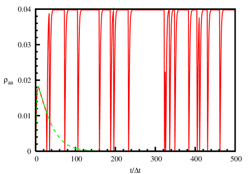
Figure 1: Typical quantum trajectories of the detector. Figure shows the probability $\rho_{aa}$ of being in the excited level of the detector. The solid line corresponds to the case when the measured system collapses to the ground state and the dashed line corresponds to the case when the measured system collapses to the excited state. The parameters used for numerical calculation are $\Delta t=0.1$, $\Gamma=10$, $\lambda=1$, and $\Omega_{D}=1$.

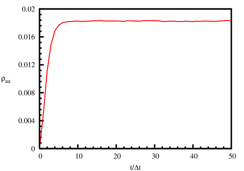
Figure 2: Probability for the detector to be in the excited state, after performing an ensemble average over 1000 trajectories. The parameters used are the same as in Fig. 1.

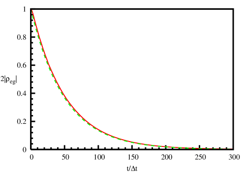
Figure 3: Non-diagonal matrix elements of the density matrix of the measured system. The solid line corresponds to the numerical calculations and the dashed line corresponds to the exponential decay with the characteristic time given by Eq. (22). The parameters used are the same as in Fig. 1.

For numerical simulation we take the measured system in an initial superposition state $\frac{1}{\sqrt{2}}(|e\rangle+|g\rangle)$. The typical quantum trajectories of the detector are shown in Fig. 1. There are two kinds of trajectories corresponding to the collapse of the measured system to the excited or the ground states. The trajectories corresponding to the collapse of the measured system to the ground state show the repeated jumps. The mean interval between jumps, obtained from the numerical simulation is of the same order of magnitude as $\tau_{M}=5$ according to Eq. (22). After averaging over the realizations the probability for the detector to be in the excited state is shown in Fig. 2. The figure shows that this probability reaches the stationary value. The time dependency of the non-diagonal matrix elements of the density matrix of the measured system is shown in Fig. 3. The figure shows a good agreement between the results of numerical calculations and the exponential decay with the characteristic time estimated from Eq. (22).

VI Frequently measured perturbed two level system

We consider an atom interacting with the classical external electromagnetic field as the measured system. Interaction of the atom with the field is described by the operator

$$\hat{V}=-\hbar\Omega_{R}(|e\rangle\langle g|+|g\rangle\langle e|)\cos\Omega t,$$ (46)

where $\Omega$ is the frequency of the field and $\Omega_{R}$ is the Rabi frequency. In the interaction representation and using the rotating-wave approximation the perturbation $\hat{V}$ is

$$\tilde{V}(t)=-\hbar\frac{\Omega_{R}}{2}(e^{i\Delta\omega t}|e\rangle\langle g|+e^{-i\Delta\omega t}|g\rangle\langle e|),$$ (47)

where

$$\Delta\omega=\omega_{A}-\Omega$$ (48)

is the detuning. Here $\hbar\omega_{A}=\hbar\omega_{e}-\hbar\omega_{g}$ is the energy difference between the excited and the ground levels of the measured atom.

If the measurements are not performed, the atom exhibits Rabi oscillations with the frequency $\Omega_{R}$. If the measured atom is initially in the state $|g\rangle$, the time dependence of the coefficient $c_{g}$ of the wavefunction $|\Psi\rangle=c_{e}|e\rangle+c_{g}|g\rangle$ is

$$c_{g}(t)=e^{-\frac{1}{2}it\Delta\omega}\left(\cos\left(\frac{1}{2}t\sqrt{\Delta\omega^{2}+\Omega_{R}^{2}}\right)+i\frac{\Delta\omega}{\sqrt{\Delta\omega^{2}+\Omega_{R}^{2}}}\sin\left(\frac{1}{2}t\sqrt{\Delta\omega^{2}+\Omega_{R}^{2}}\right)\right).$$ (49)

In particular, if the detuning $\Delta\omega$ is zero, we have

$$c_{g}(t)=c_{g}(0)\cos\left(\frac{\Omega_{R}}{2}t\right).$$ (50)

When the measured atom interacts with the detector, we take the wavefunction of the measured system and of the detector as in Eq. (39). In the interaction representation the equations for the coefficients, when the evolution is governed by the effective Hamiltonian $\hat{H}_{\mathrm{eff}}$, defined by Eq. (31), are

$$\dot{c}_{ea} = i\frac{\Omega_{R}}{2}e^{it\Delta\omega}c_{ga}-i\frac{\Omega_{D}}{2}c_{ea}-\frac{\Gamma}{2}c_{ea}$$ (51)

$$\dot{c}_{eb} = i\frac{\Omega_{R}}{2}e^{it\Delta\omega}c_{gb}+i\frac{\Omega_{D}}{2}c_{eb}$$ (52)

$$\dot{c}_{ga} = i\frac{\Omega_{R}}{2}e^{-it\Delta\omega}c_{ea}-i\lambda c_{gb}-i\frac{\Omega_{D}}{2}c_{ga}-\frac{\Gamma}{2}c_{ga}$$ (53)

$$\dot{c}_{gb} = i\frac{\Omega_{R}}{2}e^{-it\Delta\omega}c_{eb}-i\lambda c_{ga}+i\frac{\Omega_{D}}{2}c_{gb}$$ (54)

The evolution of the measured atom significantly differs from the Rabi oscillations. We are interested in the case when the duration of the measurement $\tau_{M}$ is much shorter than the period of Rabi oscillations $2\pi/\Omega_{R}$. In such a situation the non diagonal matrix elements of the density matrix of the measured system remain small and the time evolution of the diagonal matrix elements can be approximately described by the rate equations

$$\frac{d}{dt}\rho_{gg} = \Gamma_{e\rightarrow g}\rho_{ee}(t)-\Gamma_{g\rightarrow e}\rho_{gg}(t),$$ (55)

$$\frac{d}{dt}\rho_{ee} = \Gamma_{g\rightarrow e}\rho_{gg}(t)-\Gamma_{e\rightarrow g}\rho_{ee}(t).$$ (56)

If the measured atom is initially in the state $|g\rangle$, the solution of Eqs. (55) and (56) is

$$\rho_{gg}(t)=\frac{\Gamma_{e\rightarrow g}+\Gamma_{g\rightarrow e}e^{-(\Gamma_{e\rightarrow g}+\Gamma_{g\rightarrow e})t}}{\Gamma_{e\rightarrow g}+\Gamma_{g\rightarrow e}}=\frac{1}{2}\left(1+e^{-2\Gamma_{g\rightarrow e}t}\right).$$ (57)

We can estimate the rates $\Gamma_{e\rightarrow g}$ and $\Gamma_{g\rightarrow e}$ using equations from Ref. Ruseckas and Kaulakys (2004), i.e.,

$$\Gamma_{e\rightarrow g} = 2\pi\int_{-\infty}^{\infty}G(\omega)P_{eg}(\omega)d\omega,$$ (58)

$$\Gamma_{g\rightarrow e} = 2\pi\int_{-\infty}^{\infty}G(\omega)P_{ge}(\omega)d\omega,$$ (59)

where

$$P_{eg}(\omega) = \frac{1}{\pi}\mathop{\mathrm{Re}}\int_{0}^{\infty}F_{eg}(\tau)e^{i(\omega-\omega_{A})\tau}d\tau$$ (60)

$$P_{ge}(\omega) = \frac{1}{\pi}\mathop{\mathrm{Re}}\int_{0}^{\infty}F_{ge}(\tau)e^{i(\omega+\omega_{A})\tau}d\tau$$ (61)

and

$$G(\omega)=\left(\frac{\Omega_{R}}{2}\right)^{2}[\delta(\omega-\omega_{A}+\Delta\omega)+\delta(\omega+\omega_{A}-\Delta\omega)]\,.$$ (62)

Here the expression for $G(\omega)$ is derived using Eq. (47). In contrast to Ref. Ruseckas and Kaulakys (2004) in the expression for $P(\omega)$ we extended the range of the integration to the infinity since $F_{eg}(\tau)$ naturally limits the duration of the measurement. Expressions, analogous to (58), were obtained in Refs. Kofman and Kurizki (2000); Kofman et al. (2001), as well.

Using Eqs. (58)–(62) we can estimate the transition rates as

$$\Gamma_{e\rightarrow g}\approx\Gamma_{g\rightarrow e}\approx\frac{\Omega_{R}^{2}}{2}\mathop{\mathrm{Re}}\int_{0}^{\infty}F_{eg}(\tau)e^{-i\tau\Delta\omega}d\tau=\frac{\Omega_{R}^{2}}{2}\int_{0}^{\infty}e^{-\frac{\tau}{\tau_{M}}-i\tau\Delta\omega}d\tau=\frac{\Omega_{R}^{2}}{2}\frac{\tau_{M}}{1+(\tau_{M}\Delta\omega)^{2}}.$$ (63)

Here we used the expression $\exp(-\tau/\tau_{M})$ for $F_{eg}(\tau)$. When the detuning $\Delta\omega$ is zero the transition rates are

$$\Gamma_{e\rightarrow g}\approx\Gamma_{g\rightarrow e}\approx\frac{\Omega_{R}^{2}\tau_{M}}{2}.$$ (64)

The transition rates are smaller for the shorter measurements. This is a manifestation of the quantum Zeno effect.

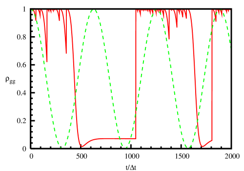
Figure 4: Typical quantum trajectory of the measured two level system (solid line). Figure shows the probability $\rho_{gg}$ for the measured atom to be in the ground level. The dashed line shows the Rabi oscillations in the measurement-free evolution. The detuning $\Delta\omega$ is zero. The parameters used for the numerical calculation are $\Delta t=0.1$, $\Gamma=10$, $\lambda=1$, $\Omega_{D}=1$, and $\Omega_{R}=0.1$.

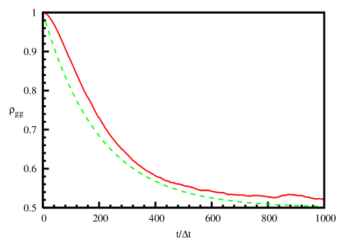
Figure 5: Probability for the measured atom to be in the ground level, after performing an ensemble average over 1000 trajectories. The solid line shows the results of the numerical calculations, the dashed line shows the approximation according to Eq. (57). The parameters used are the same as in Fig. 4.

For numerical simulation we take the measured system in an initial state $|g\rangle$. The typical quantum trajectory of the measured system is shown in Fig. 4. The behaviour of the measured system strongly differs from the measurement-free evolution. The measurement-free system oscillates with the Rabi frequency, while the measured system stays in one of the levels and suddenly jumps to the other. The probability for the measured atom to be in the ground state calculated after averaging over the realizations is shown in Fig. 5. The figure shows that this probability exhibits almost the exponential decay and after some time reaches the stationary value close to $1/2$. The figure shows a good agreement between the results of the numerical calculations and the estimate (57).

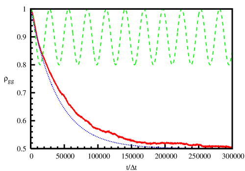
Figure 6: Probability for the atom with the nonzero detuning to be in the ground level. The solid line shows the results of the numerical simulation. The dotted line shows the approximation according to Eq. (57), using the decay rate from Eq. (63). The dashed line shows the evolution of a not measured system. The parameters used for numerical calculation are $\Delta t=0.001$, $\Gamma=10$, $\lambda=1$, $\Omega_{D}=1$, $\Omega_{R}=0.1$, and $\Delta\omega=0.2$.

When the detuning $\Delta\omega$ is not zero, the frequently measured two level system can exhibit the anti-Zeno effect. This is pointed out in Ref. Luis (2003). For the case of nonzero detuning the probability that the atom is in the ground state is shown in Fig. 6. The figure shows that the probability for the atom to be in the initial (ground) state is smaller, and, consequently, to be in the excited state is greater when the atom is measured. This is the manifestation of the quantum anti-Zeno effect in the two level system.

VII Decaying system

We model the decaying system as two level system $A$ interacting with the reservoir $F$ consisting of many levels. The full Hamiltonian of the system is

$$\hat{H}=\hat{H}_{A}+\hat{H}_{F}+\hat{V},$$ (65)

where

$$\hat{H}_{A}=\hbar\omega_{A}|e\rangle\langle e|$$ (66)

is the Hamiltonian of the two level system,

$$\hat{H}_{F}=\sum_{k}\hbar\omega_{k}|k\rangle\langle k|.$$ (67)

is the Hamiltonian of the reservoir, and

$$\hat{V}=\hbar\sum_{k}(g(k)|e\rangle\langle k|+g(k)^{*}|k\rangle\langle e|)$$ (68)

describes the interaction of the system with the reservoir, with $g(k)$ being the strength of the interaction with reservoir mode $k$. In the interaction representation the perturbation $V$ has the form

$$\tilde{V}(t)=e^{\frac{i}{\hbar}(\hat{H}_{A}+\hat{H}_{F})t}\hat{V}e^{-\frac{i}{\hbar}(\hat{H}_{A}+\hat{H}_{F})t}=\hbar\sum_{k}(g(k)e^{i(\omega_{A}-\omega_{k})t}|e\rangle\langle k|+g(k)^{*}e^{-i(\omega_{A}-\omega_{k})t}|k\rangle\langle e|).$$

The wavefunction of the system $A+F$ in the interaction representation is expressed as

$$|\tilde{\Psi}\rangle=c_{e}(t)|e\rangle|0\rangle+\sum_{k}c_{k}|g\rangle|k\rangle.$$ (69)

One can then obtain from the Schrödinger equation the following equations for the coefficients

$$\dot{c}_{e} = -i\sum_{k}g(k)e^{i(\omega_{A}-\omega_{k})t}c_{k},$$ (70)

$$\dot{c}_{k} = -ig(k)^{*}e^{-i(\omega_{A}-\omega_{k})t}c_{e}.$$ (71)

The initial condition is $|\Psi\rangle=|e\rangle|0\rangle$. Formally integrating the equation (71) we obtain the expression

$$c_{k}=-ig(k)^{*}\int_{0}^{t}e^{-i(\omega_{A}-\omega_{k})t^{\prime}}c_{e}(t^{\prime})dt^{\prime}.$$ (72)

Inserting Eq. (72) into Eq. (70), we obtain the exact integro-differential equation

$$\frac{d}{dt}c_{e}=-\int_{0}^{t}dt^{\prime}\sum_{k}|g(k)|^{2}e^{i(\omega_{A}-\omega_{k})(t-t^{\prime})}c_{e}(t^{\prime}).$$ (73)

The sum over $k$ may be replaced by an integral

$$\sum_{k}\rightarrow\int d\omega_{k}\rho(\omega_{k})$$

with $\rho(\omega_{k})$ being the density of states in the reservoir. The integration in Eq. (73) can be carried out in the Weisskopf-Wigner approximation. We get the equation

$$\frac{d}{dt}c_{e}=-\frac{\Gamma_{e\rightarrow g}^{(0)}}{2}c_{e},$$ (74)

where the decay rate $\Gamma_{e\rightarrow g}^{(0)}$ is given by the Fermi’s Golden Rule:

$$\Gamma_{e\rightarrow g}^{(0)}=2\pi\rho(\omega_{A})|g(\omega_{A})|^{2}.$$ (75)

In order to observe the quantum anti-Zeno effect one needs to have sufficiently big derivative of the quantity $\rho(\omega)|g(\omega)|^{2}$. In such a case the decay rate given by Fermi Golden Rule (75) is no longer valid. The corrected decay rate may be obtained solving Eq. (73) by the Laplace transform method Lewenstein et al. (1988). The the Laplace transform of the solution of Eq. (73) is

$$\tilde{c}_{e}(z)=\frac{1}{\mathcal{H}(z)},$$ (76)

where $\mathcal{H}(z)$ is the resolvent function

$$\mathcal{H}(z)=z+\int\frac{\rho(\omega)|g(\omega)|^{2}}{z+i(\omega-\omega_{A})}d\omega.$$ (77)

In the numerical calculations we take the frequencies of the reservoir $\omega$ distributed in the region $[\omega_{A}-\Lambda,\omega_{A}+\Lambda]$ with the constant spacing $\Delta\omega$. Therefore, the density of states is constant $\rho(\omega)=1/\Delta\omega\equiv\rho_{0}$. The simplest choice of the interaction strength $g(\omega)$ is to make it linearly dependent on $\omega$,

$$g(\omega)=g_{0}\left(1+\frac{a}{\Lambda}(\omega-\omega_{A})\right),$$ (78)

where $a$ is dimensionless parameter. Using Eq. (78) one obtains the expression for the resolvent

$$\mathcal{H}(z)=z+\pi\rho_{0}g_{0}^{2}\left[1-\frac{2}{\pi}\arctan\left(\frac{z}{\Lambda}\right)+\left(a^{2}\frac{z}{\Lambda}-i2a\right)\left(\frac{2}{\pi}-\frac{z}{\Lambda}+\frac{2}{\pi}\frac{z}{\Lambda}\arctan\left(\frac{z}{\Lambda}\right)\right)\right].$$

The real part of $z$ at which the resolvent $\mathcal{H}(z)$ is equal to zero gives the decay rate. Expanding the resolvent into the series of powers of $\Lambda^{-1}$ and keeping only the first-order terms we obtain the decay rate

$$\Gamma_{e\rightarrow g}^{(1)}\approx\Gamma_{e\rightarrow g}^{(0)}\left(1-\frac{\Gamma_{e\rightarrow g}^{(0)}}{\pi\Lambda}(5a^{2}-1)\right).$$ (79)

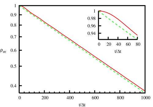
Figure 7: Time dependence of the occupation of the exited level of the decaying system. Solid line shows the results of the numerical calculation, dashed line shows the exponential decay according to the Fermi’s Golden Rule. The parameters used for the numerical calculation are $\Delta t=0.1$, $\Delta\omega=0.001$, $\Lambda=0.5$, and $g_{0}=0.001262$. For the parameters used the decay rate is $\Gamma_{e\rightarrow g}^{(0)}=0.01$.

We solve Eqs. (70) and (71) numerically, replacing them with discretized versions with the time step $\Delta t$. For calculations we used $N=1000$ levels in the reservoir. The numerical results for constant interaction strength are $g(k)=g_{0}$ presented in Fig. 7. The figure shows a good agreement between the numerical results and the exponential law according to the Fermi’s Golden Rule at intermediate times. At very short time the occupation of the excited level exhibits quadratic behaviour, which, for the repeated frequent measurements, may result in the quantum Zeno effect.

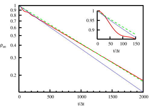
Figure 8: Time dependence of the occupation of the exited level of the decaying system when the interaction with the reservoir modes is described by Eq. (78). Solid line shows results of numerical calculation, dashed line shows exponential decay using the decay rate from Eq. (79), dotted line shows exponential decay according to Fermi’s Golden Rule (75). In the calculations we used $a=2$, other parameters are the same as in Fig. 7.

Numerical results in the case when the interaction with the reservoir modes is described by Eq. (78) with nonzero parameter $a$ are presented in Fig. 8. The figure shows good agreement between the numerical results and the exponential decay with the decay rate given by Eq. (79) at intermediate times. For very short time we observe the acceleration of the decay due to the interaction with the reservoir. This acceleration for the repeated frequent measurements results in the quantum anti-Zeno effect.

VIII Measurement of the decaying system

In this section we consider the decaying system, described in Sec. VII and interacting with the detector. The wavefunction of the measured system and the detector, when the detector interacts with the decaying system in the ground state only, we take in the form

$$|\Psi_{c}\rangle=c_{ea}|e\rangle|0\rangle|a\rangle+c_{eb}|e\rangle|0\rangle|b\rangle+\sum_{k}(c_{ka}|g\rangle|k\rangle|a\rangle+c_{kb}|g\rangle|k\rangle|b\rangle).$$ (80)

The equations for the coefficients, when the evolution is governed by the effective Hamiltonian $\hat{H}_{\mathrm{eff}}$, are

$$\dot{c}_{ea} = -i\sum_{k}g(k)e^{i(\omega_{A}-\omega_{k})t}c_{ka}-i\frac{\Omega_{D}}{2}c_{ea}-\frac{\Gamma}{2}c_{ea},$$ (81)

$$\dot{c}_{eb} = -i\sum_{k}g(k)e^{i(\omega_{A}-\omega_{k})t}c_{kb}+i\frac{\Omega_{D}}{2}c_{eb},$$ (82)

$$\dot{c}_{ka} = -ig(k)^{*}e^{-i(\omega_{A}-\omega_{k})t}c_{ea}-i\lambda c_{kb}-i\frac{\Omega_{D}}{2}c_{ka}-\frac{\Gamma}{2}c_{ka},$$ (83)

$$\dot{c}_{kb} = -ig(k)^{*}e^{-i(\omega_{A}-\omega_{k})t}c_{eb}-i\lambda c_{ka}+i\frac{\Omega_{D}}{2}c_{kb}.$$ (84)

After the jump in the detecting atom the unnormalized wavefunction becomes

$$\hat{C}|\Psi_{c}\rangle=\sqrt{\Gamma}(c_{ea}|e\rangle|0\rangle|b\rangle+\sum_{k}c_{ka}|g\rangle|k\rangle|b\rangle).$$ (85)

According to Ref. Ruseckas and Kaulakys (2004), the decay rate of the measured system is given by expression (58) with

$$G(\omega)=\rho(\omega)|g(\omega)|^{2}$$ (86)

and

$$P(\omega)=\frac{1}{\pi}\mathop{\mathrm{Re}}\int_{0}^{\infty}F_{eg}(\tau)e^{i(\omega-\omega_{A})\tau}d\tau.$$ (87)

Using $F_{eg}(\tau)=\exp(-\tau/\tau_{M})$ we obtain

$$P(\omega)=\frac{1}{\pi}\frac{\tau_{M}}{1+(\omega-\omega_{A})^{2}\tau_{M}^{2}}.$$ (88)

In order to obtain the quantum Zeno effect we take $G(\omega)$ as a constant

$$G(\omega)=\frac{\hbar^{2}g_{0}^{2}}{\Delta\omega},\quad\omega_{A}-\Lambda\leq\omega\leq\omega_{A}+\Lambda.$$ (89)

Here $\Delta\omega$ is the spacing between the modes of the reservoir. Using Eq. (58) we get the decay rate of the measured decaying system

$$\Gamma_{e\rightarrow g}=\Gamma_{e\rightarrow g}^{(0)}\frac{2}{\pi}\arctan(\Lambda\tau_{M}).$$ (90)

When $\Lambda\tau_{M}$ is big, we obtain the expression

$$\Gamma_{e\rightarrow g}=\Gamma_{e\rightarrow g}^{(0)}\left(1-\frac{2}{\pi}\frac{1}{\Lambda\tau_{M}}+\cdots\right)$$ (91)

by expanding Eq. (90) into series of the powers of $(\Lambda\tau_{M})^{-1}$. The second term in Eq. (91) shows that the decay rate decreases with the decreasing duration of the measurement $\tau_{M}$. This is the manifestation of the quantum Zeno effect.

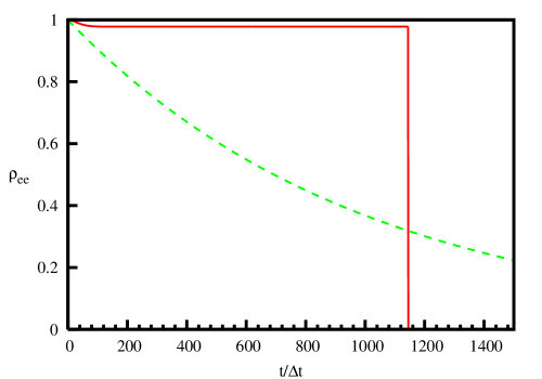
Figure 9: Typical quantum trajectory (solid line) of the measured decaying system when the detector interacts with the ground state of the measured system. Figure shows the probability $\rho_{ee}$ that the measured atom is in the excited level. The dashed line shows the exponential decay according to the Fermi’s Golden Rule in the measurement-free evolution. The parameters used for the numerical calculation are $\Delta t=0.1$, $\Gamma=10$, $\lambda=1$, $\Omega_{D}=1$, $\Delta\omega=0.001$, $\Lambda=0.5$, and $g_{0}=0.001262$. For the parameters used the decay rate is $\Gamma_{e\rightarrow g}=0.01$.

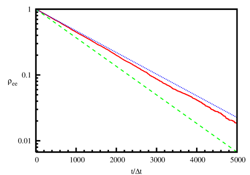
Figure 10: Time dependence of the occupation of the exited level of the decaying system. Solid line shows results of numerical calculation, dashed line shows exponential decay according to Fermi’s Golden Rule. The dotted line shows approximation according to Eq. (90). The parameters used are the same as in Fig. 9.

The results of the numerical simulation are presented in Figs. 9 and 10. Typical quantum trajectory of the measured decaying system is shown in Fig. 9. This trajectory is compatible with the intuitive quantum jump picture: the system stays in the excited state for some time and then suddenly jumps to the ground state. The probability that the measured system stays in the excited state is presented in Fig. 10. Figure shows a good agreement between the numerical simulation and the exponential law approximation with the exponent given in Eq. (90). Also the quantum Zeno effect is apparent.

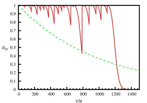
Figure 11: Typical quantum trajectory of the measured decaying system (solid line) when the detector interacts with the excited level. Figure shows the probability $\rho_{ee}$ that the measured atom is in the excited level. The dashed line shows exponential decay according to the Fermi’s Golden Rule in the measurement-free evolution. The parameters used are the same as in Fig. 9.

When the detector interacts with the excited state of the decaying system the interaction term is

$$\hat{H}_{I}=\hbar\lambda|e\rangle\langle e|(\hat{\sigma}_{+}+\hat{\sigma}_{-})$$ (92)

and the quantum trajectories are different. Typical quantum trajectory is shown in Fig. 11. This difference can be explained in the following way: when the detector interacts with the ground state, the interaction effectively begins only after some time, when the probability to find the system in the ground state is sufficiently big. This explains the absence of the collapses at short times in Fig. 9. Then, the measurement result after the collapse most likely will be that the system is found in the ground state. When the detector interacts with the excited state of the system, the interaction starts immediately and soon after that the most probable result of the measurement is that the measured system is in the excited state. It should be noted, that the averaged evolution shown in Fig. 10 does not depend on the state the detector is interacting.

The model used for the decaying system when $g(\omega)=\mathrm{const}$ does not allow to obtain the quantum anti-Zeno effect, since the conditions for the quantum anti-Zeno effect, presented in Ref. Kofman and Kurizki (2000), are not satisfied. In order to obtain the quantum ant-Zeno effect we use the interaction with the reservoir modes described by Eq. (78). In such a case we have

$$G(\omega)=\frac{\hbar^{2}g_{0}^{2}}{\Delta\omega}\left(1+\frac{a}{\Lambda}(\omega-\omega_{A})\right)^{2},\quad\omega_{A}-\Lambda\leq\omega\leq\omega_{A}+\Lambda.$$ (93)

Equation (58) in this case does not give correct decay rate of the measured system. In order to estimate the decay rate, we solve the Liouville-von Neumann equation $i\hbar\dot{\rho}=[\hat{H},\rho]$ for the density matrix of the system with the Hamiltonian (65)–(68), including additional terms describing decay of the non-diagonal elements with rate $1/\tau_{M}$, i.e.,

$$\dot{\rho}_{e0,e0} = -i\sum_{k}(g(k)\rho_{gk,e0}-\rho_{e0,gk}g(k)^{*}),$$ (94)

$$\dot{\rho}_{gk,gk^{\prime}} = -i\omega_{kk^{\prime}}\rho_{gk,gk^{\prime}}-i(g(k)^{*}\rho_{e0,gk^{\prime}}-\rho_{gk,e0}g(k^{\prime})),$$ (95)

$$\dot{\rho}_{e0,gk} = \left(-i(\omega_{A}-\omega_{k})-\frac{1}{\tau_{M}}\right)\rho_{e0,gk}-i(\sum_{k^{\prime}}g(k^{\prime})\rho_{gk^{\prime},gk}-\rho_{e0,e0}g(k)),$$ (96)

$$\dot{\rho}_{gk,e0} = \left(-i(\omega_{k}-\omega_{A})-\frac{1}{\tau_{M}}\right)\rho_{gk,e0}-i(g(k)^{*}\rho_{e0,e0}-\sum_{k^{\prime}}\rho_{gk,gk^{\prime}}g(k^{\prime})^{*}).$$ (97)

We solve equations (94)–(97) using the Laplace transform method. Eliminating $\tilde{\rho}_{e0,gk}$ and $\tilde{\rho}_{gk,e0}$ from the Laplace transform of Eqs. (94)–(97) one gets the equations for the Laplace transforms of the matrix elements of the density matrix,

$$z\tilde{\rho}_{e0,e0}(z)-1 = -\sum_{k}|g(k)|^{2}\left(\frac{1}{z+i(\omega_{k}-\omega_{A})+\frac{1}{\tau_{M}}}+\frac{1}{z+i(\omega_{A}-\omega_{k})+\frac{1}{\tau_{M}}}\right)\tilde{\rho}_{e0,e0}(z)$$ (98)

$$+\sum_{k,k^{\prime}}\left(\frac{1}{z+i(\omega_{k}-\omega_{A})+\frac{1}{\tau_{M}}}+\frac{1}{z+i(\omega_{A}-\omega_{k^{\prime}})+\frac{1}{\tau_{M}}}\right)$$

$$\times g(k)g(k^{\prime})^{*}\tilde{\rho}_{gk,gk^{\prime}}(z),$$

$$(z+i\omega_{kk^{\prime}})\tilde{\rho}_{gk,gk^{\prime}}(z) = -\sum_{k^{\prime\prime}}\left(\frac{g(k^{\prime})g(k^{\prime\prime})^{*}}{z+i(\omega_{k}-\omega_{A})+\frac{1}{\tau_{M}}}\tilde{\rho}_{gk,gk^{\prime\prime}}(z)+\frac{g(k^{\prime\prime})g(k)^{*}}{z+i(\omega_{A}-\omega_{k^{\prime}})+\frac{1}{\tau_{M}}}\tilde{\rho}_{gk^{\prime\prime},gk^{\prime}}(z)\right)$$ (99)

$$+g(k^{\prime})g(k)^{*}\left(\frac{1}{z+i(\omega_{k}-\omega_{A})+\frac{1}{\tau_{M}}}+\frac{1}{z+i(\omega_{A}-\omega_{k^{\prime}})+\frac{1}{\tau_{M}}}\right)\tilde{\rho}_{e0,e0}(z).$$

On the r.h.s. of Eq. (99) we will neglect the small terms not containing $\tilde{\rho}_{e0,e0}(z)$. Expressing $\tilde{\rho}_{gk,gk^{\prime}}(z)$ via $\tilde{\rho}_{e0,e0}(z)$ from Eq. (99), substituting into Eq. (98) and replacing the sum over $k$ by an integral we obtain

$$\frac{1}{\tilde{\rho}_{e0,e0}(z)} = z+\int d\omega G(\omega)\left(\frac{1}{z+i(\omega-\omega_{A})+\frac{1}{\tau_{M}}}+\frac{1}{z+i(\omega_{A}-\omega)+\frac{1}{\tau_{M}}}\right)$$ (100)

$$-\int d\omega\int d\omega^{\prime}G(\omega)G(\omega^{\prime})\frac{1}{z+i(\omega-\omega^{\prime})}$$

$$\times\left(\frac{1}{z+i(\omega-\omega_{A})+\frac{1}{\tau_{M}}}+\frac{1}{z+i(\omega_{A}-\omega^{\prime})+\frac{1}{\tau_{M}}}\right)^{2}\,.$$

The value of $z$ at which the r.h.s of Eq. (100) is equal to zero gives the decay rate. Using the expression (93) for $G(\omega)$ and keeping only the first-order terms of the expansion into series of the powers of $\Lambda^{-1}$ we get the measurement-modified decay rate

$$\Gamma_{e\rightarrow g}=\Gamma_{e\rightarrow g}^{(0)}\left(1-\frac{\Gamma_{e\rightarrow g}^{(0)}}{\pi\Lambda}(5a^{2}-1)\right)+\Gamma_{e\rightarrow g}^{(0)}\frac{2}{\pi}\frac{(a^{2}-1)}{\Lambda\tau_{M}}.$$ (101)

Equation (101) is valid only for sufficiently large duration of the measurement $\tau_{M}$, since expansion into series requires that $\Lambda\tau_{M}\gg 1$. From Eq. (101) one can see that in order to obtain the quantum anti-Zeno effect the parameter $a$ should be greater than $1$. When the parameter $a$ is less than $1$ we get the Zeno effect, and when $a=1$ the decay rate coincides with the decay rate of the free system.

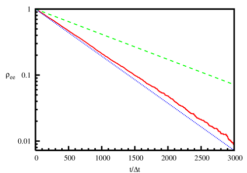
Figure 12: Time dependence of the occupation of the exited level of the decaying system when the interaction with the reservoir modes is described by Eq. (78). Solid line shows results of the numerical calculation, dashed line shows exponential decay of the measurement-free system with the decay rate given by Eq. (79). The dotted line shows approximation according to Eq. (101). In the calculations we used $a=2$, while other parameters are the same as in Fig. 9.

The probability that the measured system stays in the excited state, obtained from numerical simulation is presented in Fig. 12. Figure clearly demonstrates the quantum anti-Zeno effect, the decay rate of the measured system is bigger than that of the measurement-free system.

IX Conclusions

We model the evolution of the measured quantum system as a detector using a two level system interacting with the environment. The influence of the environment is taken into account using quantum trajectory method. The quantum trajectories produced by stochastic simulations show the probabilistic behavior exhibiting the collapse of the wave-packet in the measured system, although the quantum jumps were performed only in the detector. Both quantum Zeno and anti-Zeno effects were demonstrated for the measured two level system and for the decaying system.

The results of the numerical calculations are compared with the analytical expressions for the decay rate of the measured system. It is found that the general expression (58), obtained in Ref. Ruseckas and Kaulakys (2004), gives good agreement with the numerical data for the measured two level system and for the decaying one showing the quantum Zeno effect. Nevertheless, when the interaction of the measured system with the reservoir is strongly mode-dependent, this expression does not give the correct decay rate. The decay rate in this case was estimated including additional terms describing decay of non-diagonal elements into the equation for the density matrix of the measured system and a good agreement with the numerical calculations is found. A good agreement of the numerical results with the analytical estimates of the decay rates of the measured system shows that the particular model of the detector is not important, since the decay rates mostly depend only on one parameter, i.e., the duration of the measurement (22).

References

- Khalfin (1958) L. A. Khalfin, Sov. Phys. JETP 6, 1503 (1958).
- Wilkinson et al. (1997) S. R. Wilkinson, C. F. Bharucha, M. C. Fisher, K. W. Mardison, P. R. Morrow, Q. Niu, B. Sundaram, and M. G. Raizen, Nature (London) 387, 575 (1997).
- Mishra and Sudarshan (1977) B. Mishra and E. C. G. Sudarshan, J. Math. Phys. 18, 756 (1977).
- Itano et al. (1990) W. M. Itano, D. J. Heinzen, J. J. Bollinger, and D. J. Wineland, Phys. Rev. A 41, 2295 (1990).
- Kwiat et al. (1995) P. Kwiat, H. Weinfurter, T. Herzog, A. Zeilinger, and M. A. Kasevich, Phys. Rev. Lett. 74, 4763 (1995).
- Nagels et al. (1997) B. Nagels, L. J. F. Hermans, and P. L. Chapovsky, Phys. Rev. Lett. 79, 3097 (1997).
- Toschek and Wunderlich (2001) P. E. Toschek and C. Wunderlich, Eur. Phys. J. D 14, 387 (2001).
- Kaulakys and Gontis (1997) B. Kaulakys and V. Gontis, Phys. Rev. A 56, 1131 (1997).
- Kofman and Kurizki (2000) A. G. Kofman and G. Kurizki, Nature (London) 405, 546 (2000).
- Lewenstein and Rza̧žewski (2000) M. Lewenstein and K. Rza̧žewski, Phys. Rev. A 61, 022105 (2000).
- Facchi et al. (2001) P. Facchi, H. Nakazato, and S. Pascazio, Phys. Rev. Lett. 86, 2699 (2001).
- Ruseckas and Kaulakys (2001) J. Ruseckas and B. Kaulakys, Phys. Rev. A 63, 062103 (2001).
- Kofman et al. (2001) A. G. Kofman, G. Kurizki, and T. Opatrny, Phys. Rev. A 63, 042108 (2001).
- Fischer et al. (2001) M. C. Fischer, B. Gutiérrez-Medina, and M. G. Raizen, Phys. Rev. Lett. 87, 040402 (2001).
- Facchi and Pascazio (2002) P. Facchi and S. Pascazio, Phys. Rev. Lett. 89, 080401 (2002).
- Facchi and Pascazio (2001) P. Facchi and S. Pascazio, Progr. Opt. 42, 147 (2001).
- Simonius (1978) M. Simonius, Phys. Rev. Lett. 40, 980 (1978).
- Harris and Stodolsky (1982) R. A. Harris and L. Stodolsky, Phys. Lett. 116B, 464 (1982).
- Schulman (1998) L. S. Schulman, Phys. Rev. A 57, 1509 (1998).
- Panov (1999) A. D. Panov, Phys. Lett. A 260, 441 (1999).
- Mensky (1999) M. B. Mensky, Phys. Lett. A 257, 227 (1999).
- Petrosky et al. (1990) T. Petrosky, S. Tasaki, and I. Prigogine, Phys. Lett. A 151, 109 (1990).
- Frerichs and Schenzle (1991) V. Frerichs and A. Schenzle, Phys. Rev. A 44, 1962 (1991).
- Pascazio and Namiki (1994) S. Pascazio and M. Namiki, Phys. Rev. A 50, 4582 (1994).
- Zurek (1984) W. H. Zurek, Phys. Rev. Lett. 53, 391 (1984).
- Vaidman et al. (1996) L. Vaidman, L. Goldenberg, and S. Wiesner, Phys. Rev. A 54, R1745 (1996).
- Beige (2004) A. Beige, Phys. Rev. A 69, 012303 (2004).
- Erez et al. (2004) N. Erez, Y. Aharonov, B. Reznik, and L. Vaidman, Phys. Rev. A 69, 062315 (2004).
- Franson et al. (2004) J. D. Franson, B. C. Jacobs, and T. B. Pittman, Phys. Rev. A 70, 062302 (2004).
- Brion et al. (2005) E. Brion, V. M.Akulin, D. Comparat, I. Dumer, G. Harel, N. Kébaili, G. Kurizki, I. Mazets, and P. Pillet, Phys. Rev. A 71, 052311 (2005).
- Zurek (1981) W. H. Zurek, Phys. Rev. D 24, 1516 (1981).
- Zurek (1982) W. H. Zurek, Phys. Rev. D 26, 1862 (1982).
- Walls et al. (1985) D. F. Walls, M. J. Collet, and G. J. Milburn, Phys. Rev. D 32, 3208 (1985).
- Unruh and Zurek (1989) W. G. Unruh and W. H. Zurek, Phys. Rev. D 40, 1071 (1989).
- Zurek (1991) W. H. Zurek, Phys. Today 44, 36 (1991), and references therein.
- Walls and Milburn (1994) D. F. Walls and G. J. Milburn, Quantum Optics (Springer, Berlin, 1994).
- Guilini et al. (1996) D. Guilini, E. Joos, C. Keffer, J. Kupsh, I. O. Stamatescu, and H. D. Zeh, Decoherence and the Appearance of a Classical World in Quantum Theory (Springer, New York, 1996).
- Carmichael (1993) H. Carmichael, An Open Systems Approach to Quantum Optics (Springer-Verlag, 1993).
- Dalibard et al. (1992) J. Dalibard, Y. Castin, and K. Mølmer, Phys. Rev. Lett. 68, 580 (1992).
- Gisin and Percival (1992) N. Gisin and I. C. Percival, J. Phys. A 25, 5677 (1992).
- Hegerfeldt (1993) G. C. Hegerfeldt, Phys. Rev. A 47, 449 (1993).
- Mølmer et al. (1993) K. Mølmer, Y. Castin, and J. Dalibard, J. Opt. Soc. Am. B 10, 524 (1993).
- Power and Knight (1996) W. L. Power and P. L. Knight, Phys. Rev. A 53, 1052 (1996).
- Unruh (1979) W. G. Unruh, Phys. Rev. D 19, 2888 (1979).
- Caves et al. (1980) C. M. Caves, K. S. Thorne, R. W. P. Drever, V. D. Sandberg, and M. Zimmermann, Rev. Mod. Phys. 57, 341 (1980).
- Braginsky et al. (1980) V. B. Braginsky, Y. I. Vorontsov, and K. S. Thorne, Science 209, 547 (1980).
- Braginsky and Khalili (1996) V. B. Braginsky and F. Y. Khalili, Rev. Mod. Phys. 68, 1 (1996).
- Dum et al. (1992) R. Dum, P. Zoller, and H. Ritsch, Phys. Rev. A 45, 4879 (1992).
- Gardiner et al. (1992) C. W. Gardiner, A. S. Parkins, and P. Zoller, Phys. Rev. A 46, 4363 (1992).
- Gisin (1984) N. Gisin, Phys. Rev. Lett. 52, 1657 (1984).
- Schack et al. (1995) R. Schack, T. A. Brun, and I. C. Percival, J. Phys. A 28, 5401 (1995).
- Ruseckas and Kaulakys (2004) J. Ruseckas and B. Kaulakys, Phys. Rev. A 69, 032104 (2004).
- Luis (2003) A. Luis, Phys. Rev. A 67, 062113 (2003).
- Lewenstein et al. (1988) M. Lewenstein, J. Zakrzewski, and T. W. Mossberg, Phys. Rev. A 38, 808 (1988).