Photon Distribution Function for Long-Distance Propagation of Partially Coherent Beams through the Turbulent Atmosphere

Abstract

The photon density operator function is used to calculate light beam propagation through turbulent atmosphere. A kinetic equation for the photon distribution function is derived and solved using the method of characteristics. Optical wave correlations are described in terms of photon trajectories that depend on fluctuations of the refractive index. It is shown that both linear and quadratic disturbances produce sizable effects for long-distance propagation. The quadratic terms are shown to suppress the correlation of waves with different wave vectors.

We examine the intensity fluctuations of partially coherent beams (beams whose initial spatial coherence is partially destroyed). Our calculations show that it is possible to significantly reduce the intensity fluctuations by using a partially coherent beam. The physical mechanism responsible for this pronounced reduction is similar to that of the Hanbury-Braun, Twiss effect.

LAUR-06-1605

1 Introduction

The study of the interaction of light beams with a random media is of great importance for applications in such areas as astronomy, laser communication, laser radar systems, etc. Fluctuations of the atmospheric refractive index, caused by turbulent eddies, affect electromagnetic waves. The effects of turbulence have been investigated both theoretically and experimentally over the past few decades. (See, for example, the monographs [1]-[3] and the surveys [4]-[7].) Additional beam spreading, beam wandering (“dancing”), intensity fluctuations (known as “scintillations”), etc. caused by turbulence limit significantly the range and the performance of free-space communication systems.

It has been established that coherent laser beams are very sensitive to atmospheric conditions. Realizing this, the idea of utilizing of partially coherent beams (PCB) for practical purposes has arisen. It was shown by numerous researchers (see, for example, publications [8]-[14]) that partially coherent beams are less affected by turbulence than fully coherent beams. A specific case (in which the spatial coherence of the signal-carrying laser beam is partially destroyed before it is launched into the atmospheric channel) was considered by many researchers. This beam has the angular spread in free space of the order of $\lambda/l_{c}$ ($\lambda$ and $l_{c}$ are the wavelength and the transverse correlation length of phase distortion at the source aperture, respectively), which is larger than that of the coherent beam. For not too large distances of propagation, beam spreading due to the small initial coherence length, $l_{c}$, may dominate throughout the trajectory. One can say that the effects of turbulence are masked by the larger initial free-space spreading. At the same time it is evident that, with increasing propagation distance, the atmospheric inhomogeneity becomes the dominating factor. This results in a beam size that is almost independent of the initial correlation length.

The dependence of the intensity fluctuations on the initial coherence is more intricate than the dependence of beam spreading. Provided the dependence of the intensity fluctuations on the initial coherence is given, the noise/signal ratio can be controlled by choosing the optimal initial coherence length, $l_{c}$. This tempting opportunity has stimulated many studies in this field [9], [15]-[21]. It was shown that control is possible for small fluctuations (weak turbulence or short-distance propagation).

At moderate and strong fluctuations the situation is more complicated. Banakh et al. [18] have shown that for long distances of propagation or for strong turbulence the intensity fluctuations have a tendency to saturate at a level which depends on the initial spatial coherence. This level may be much lower than that of the coherent beam by the factor, $(r_{0}/l_{c})^{2}$, where $r_{0}$ is the initial radius of the beam. The paper deals with the physical model when the measuring device (detector) has the response time, $\tau_{d}$, greater than the coherence time, $\tau_{s}$, of the radiation at the beginning of the trajectory. In this case, the detector averages the signal over the initial fluctuations, which are due to temporal intensity fluctuations of the source and (or) may be generated when a coherent beam is transformed into PCB. The authors of [18] have solved an equation for the fourth-order coherence function (the fourth moment of the field). The derivation of the equation for fourth moment in the limit of Markov approximation is given in [1], [4]. Its solution is based on the approximate method developed by Yakushkin in [22]. The authors of [18] have modified the Yakushkin approach to be applicable to the case of PCB. The Yakushkin method is based on the observation that, for long distance propagation, the dominant contribution to the fourth-order correlation function comes from the products of two second-order coherence functions just as if Gaussian statistics for radiation field were valid. The Dashen analysis [23] in terms of the path integral formalism and the results of Fante [24] obtained by employing the extended Huygens-Fresnel principle have justified the Yakushkin idea. It seems to be quite reasonable to consider that after long-distance propagation through a medium with a random refractive index, the statistics of the photon flux acquires some of the properties of thermal radiation.

For similar conditions, when the coherence time of the quasimonochromatic laser source is much smaller than the detector’s integration time interval, $\tau_{d}$, Korotkova et al. [21] have derived an analytical expression (see Eq. (33) in [21]) for the intensity fluctuations. The paper [21] has generalized the analytical approach developed by Andrews and Phillips (see monographs [2] and [3]) to the case of PCB. This approach is a modification of the Rytov theory. Namely, in addition to the first-order perturbation of the complex phase of the field caused by refractive index fluctuations (as in Rytov theory), second-order perturbation terms are taken into account. The results of [21] differs from those in [18]. More comments are presented in Section 4.

The purpose of our paper is to develop a new quantum perturbation theory based on path integrals. This approach allows us to obtain the scintillation index for the case of a PCB, including a limit of a strong turbulence and long-distance propagation. Our approach uses the distribution function of photons (for photon density in phase space), $f({\bf r},{\bf q},t)$, where ${\bf r}$ and ${\bf q}$ are the coordinate and the momentum of photon, to describe the beam characteristics at an arbitrary instant, $t$. The first and second moments of the distribution function ($<f>$ and $<ff>$) are used to obtain the beam size and intensity fluctuations, respectively. Also, higher-order moments will be obtained for long propagation paths.

The next Section deals with the definition of the distribution function. The equation governing the evolution of the distribution function will be derived.

2 The photon distribution function and its evolution

The Hamiltonian of photons in a medium with a fluctuating refractive index is given by

$$H=\sum_{\bf k}\hbar\omega_{\bf k}b^{+}_{\bf k}b_{\bf k}-\sum_{{\bf k},{\bf k^{\prime}}}\hbar\omega_{\bf k}n_{\bf k^{\prime}}b^{+}_{\bf k}b_{{\bf k}+{\bf k^{\prime}}},$$ (1)

where the two terms on the right-hand side describe photons in a vacuum and the effect of refractive index fluctuations, respectively; $b^{+}_{\bf k}$ and $b_{\bf k}$ are creation and annihilation operators of photons with momentum ${\bf k}$, $\hbar\omega_{\bf k}\equiv\hbar ck$ is the photon energy, $c$ is the speed of light in a vacuum, and $n_{\bf k}$ is the Fourier transform of the refractive index fluctuations $\delta n({\bf r})$. The Fourier transform is defined by

$$n_{\bf k}=\frac{1}{V}\int dVe^{i{\bf kr}}\delta n({\bf r}),$$ (2)

were $V\equiv L_{x}L_{y}L_{z}$ is the normalizing volume.

Eq. (1) follows from the representation of the energy of the random medium + electromagnetic field given in [25] (Chapter 15) in the limit of small wave-vectors ${\bf{k^{\prime}}}$ ($k^{\prime}\ll k$) and of atmosphere refractive index close to unity ($n({\bf r})-1<<1$). The former means that the scale of spatial inhomogeneity of turbulence is much greater than the wavelength of the radiation. For simplicity, we consider here only the case of polarized light with a fixed polarization throughout the distance of propagation. Depolarization effects due to atmosphere turbulence are very small. (See, for example, papers [26] and [27].) Also, the terms describing the zero-point electromagnetic energy are omitted in Eq. (1).

The photon distribution function is defined by analogy with the distribution functions for electrons, phonons [28], etc. It is given by

$$f({\bf r},{\bf q},t)=\frac{1}{V}\sum_{\bf k}e^{-i{\bf kr}}b^{+}_{{\bf q}+{\bf k}/2}b_{{\bf q}-{\bf k}/2},$$ (3)

The distribution function will be used to describe beams with characteristic sizes much larger than the photon wave-length. Thus, we will restrict a sum over ${\bf k}$ by some $k_{0}$ ($k<k_{0}<<q_{0}$, where $q_{0}$ is the wave vector corresponding to the central frequency $\omega_{0}$ of radiation, $\omega_{0}=cq_{0}$). At the same time $k_{0}$ is chosen to be large enough to sample the spatial variation of the light intensity.

After integration of the operator function $f({\bf r},{\bf q},t)$ over the volume $V$, we obtain the operator for the total number of photons with momentum ${\bf q}$:

$$\int dVf({\bf r},{\bf q},t)=b^{+}_{\bf q}b_{\bf q}.$$ (4)

Similarly, the quantity obtained after a summation of $f({\bf r},{\bf q},t)$ over ${\bf q}$ may serve as a photon density averaged over a small spatial area with the size $\pi/k_{0}$. This is very similar to the Mandel operator [29] (Chapter 12) introduced in [30].

Here and in the remainder of this paper, we use the Heisenberg representation for all operators. Thus, the evolution of $f({\bf r},{\bf q},t)$ is determined by the commutator with the total Hamiltonian:

$$\partial_{t}f{\bf r},{\bf q},t)=\frac{1}{i\hbar}[f{\bf r},{\bf q},t),H].$$ (5)

Eq. (5) can be written explicitly as

$$\partial_{t}f({\bf r},{\bf q},t)+{\bf c_{q}}\partial_{\bf r}f({\bf r},{\bf q},t)-i\omega_{0}\sum_{\bf k}e^{-i{\bf kr}}n_{\bf k}\Bigg{[}f\Bigg{(}{\bf r},{\bf q}+\frac{\bf k}{2},t\Bigg{)}-f\Bigg{(}{\bf r},{\bf q}-\frac{\bf k}{2},t\Bigg{)}\Bigg{]}=0,$$ (6)

where ${\bf c_{q}}=\partial_{\bf q}\omega_{\bf q}$.

Considering the characteristic values of the photon momentum to be much greater than the wave vectors of turbulence, we can express the difference of functions in square brackets by the corresponding derivative. A detailed discussion of this approximation is given in Section 6. Then, after summing over ${\bf k}$, we obtain

$$\{\partial_{t}+{\bf c_{q}}\partial_{\bf r}+{\bf F}({\bf r})\partial_{\bf q}\}f({\bf r},{\bf q},t)=0,$$ (7)

where ${\bf F}({\bf r})=\omega_{0}\partial_{\bf r}n({\bf r})$. As we see, the photon distribution function is governed by a kinetic equation in which the random force ${\bf F}({\bf r})$ originates from atmospheric turbulence.

The distribution function determines density of photons at a point (${\bf r}$,${\bf q}$) of the phase space at time $t$. Eq. (7) may be interpreted as the equation governing the evolution of a particle distribution function in which the state of each particle is described by the individual coordinate ${\bf r}$ and the momentum ${\bf q}$. The trajectories of these particles may be obtained from the solution of the equations of motion:

$$\frac{\partial{\bf r}(t)}{\partial t}={\bf c}({\bf q}(t)),$$

$$\frac{\partial{\bf q}(t)}{\partial t}={\bf F}({\bf r}(t)).$$ (8)

Then, the general solution of Eq. (7) is given by

$$f({\bf r},{\bf q},t)=\phi\Bigg{\{}{\bf r}-\int_{0}^{t}dt^{\prime}\frac{\partial{\bf r}(t^{\prime})}{\partial t^{\prime}};{\bf q}-\int_{0}^{t}dt^{\prime}\frac{\partial{\bf q}(t^{\prime})}{\partial t^{\prime}}\Bigg{\}},$$ (9)

where the function $\phi({\bf r},{\bf q})$ is the “initial” value of $f({\bf r},{\bf q},t)$, i.e.

$$\phi({\bf r},{\bf q})=\frac{1}{V}\sum_{\bf k}e^{-i{\bf kr}}(b^{+}_{{\bf q}+{\bf k}/2}b_{{\bf q}-{\bf k}/2})|_{t=0}\equiv\sum_{\bf k}e^{-i{\bf kr}}\phi({\bf k},{\bf q}),$$ (10)

and the “trajectories” ${\bf r}(t^{\prime})$ and ${\bf q}(t^{\prime})$ pass through the point ${\bf r},{\bf q}$ at $t^{\prime}=t$ [i.e. ${\bf r}(t^{\prime}=t)={\bf r},{\bf q}(t^{\prime}=t)={\bf q})$]. As one can see, the photon distribution function at an arbitrary instant $t$ is expressed via the operators $b^{+}_{\bf q},b_{\bf q}$ defined for some fixed $t_{0}$ ($t_{0}$ is chosen to be equal to $0$ in Eq. (9). It is convenient to put $t-t_{0}=z/c$. Thus, $t_{0}$ is the instant when photons exit from the source. The initial photon statistics (at $t_{0}$), determined by the source properties, is assumed to be given.

We consider here the propagation of light beams with narrow spread (paraxial beams). In this case, $k_{\bot},q_{\bot}\ll q_{0}$, where index (_⊥) means perpendicular to the direction of propagation (the $z$-axis) components. The relative effect of turbulence on $q_{z}$ is negligible because of the large value of $q_{0}$. At the same time, $q_{\bot}$, which determines a beam divergence, can be increased considerably due to turbulence (compared to the initial value). Therefore, beam characteristics should be modified significantly for the case of long distance propagation.

It follows from Eq. (8) that the evolution of transverse photon momentum is given by

$${\bf q}_{\bot}(t^{\prime})={\bf q}_{\bot}+\int_{t}^{t^{\prime}}dt^{\prime\prime}{\bf F}_{\bot}[{\bf r}(t^{\prime\prime})].$$ (11)

Similarly, we obtain an expression for ${\bf r}(t^{\prime})$

$${\bf r}(t^{\prime})={\bf r}-{\bf c_{q}}(t-t^{\prime})-\frac{c}{q_{0}}\int_{t}^{t^{\prime}}dt^{\prime\prime}(t^{\prime\prime}-t^{\prime}){\bf F}_{\bot}[{\bf r}(t^{\prime\prime})].$$ (12)

Then, Eq. (9) can be written as

$$f({\bf r},{\bf q},t)=\phi\Bigg{\{}{\bf r}-{\bf c_{q}}t+\frac{c}{q_{0}}\int_{0}^{t}dt^{\prime}t^{\prime}{\bf F}_{\bot}[{\bf r}(t^{\prime})];{\bf q}-\int_{0}^{t}dt^{\prime}{\bf F}_{\bot}[{\bf r}(t^{\prime})]\Bigg{\}}.$$ (13)

A regular iterative procedure is applicable here to expand ${\bf r}(t^{\prime})$ in powers of ${\bf F}$. Then, substituting the explicit terms ${\bf r}(t^{\prime})$ into Eq. (13), we will obtain solution of the problem. In particular, the first and second moments of $f$, which describe beam spreading and intensity fluctuation, can be calculated. Applying this perturbation method, we can investigate the effects of the initial partial (spatial) coherence on beam spreading and scintillations.

3 Beam spread and intensity fluctuations

The intensity of radiation in the $z$-direction at ${\bf r}$ can be presented in the form

$$I({\bf r})=c\sum_{\bf q}\hbar\omega_{\bf q}f({\bf r},{\bf q},t).$$ (14)

This can be rewritten as

$$I({\bf r})=c\hbar\omega_{0}\sum_{\bf q,k}e^{-i{\bf k}\{{\bf r}-{\bf c}({\bf q})t+(c/q_{0})\int_{0}^{t}dt^{\prime}t^{\prime}{\bf F}_{\bot}[{\bf r}(t^{\prime})]\}}\phi_{\bf k}\Bigg{\{}{\bf q}-\int_{0}^{t}dt^{\prime}t^{\prime}{\bf F}_{\bot}[{\bf r}(t^{\prime})]\Bigg{\}}.$$ (15)

Let us restrict ouselves to only linear in ${\bf F}$ terms in Eq. (12). In other words, we put ${\bf r}-{\bf c_{q}}(t-t^{\prime})$ for ${\bf r}(t^{\prime})$ in arguments of ${\bf F}_{\bot}$ of Eq. (15). After changing variables ${\bf q}_{\bot}-\int_{0}^{t}dt^{\prime}t^{\prime}{\bf F}_{\bot}[{\bf r}(t^{\prime})]\rightarrow{\bf q}_{\bot}$ and using the relation $z=ct$, Eq. (15) is transformed to

$$I({\bf r})=c\hbar\omega_{0}\sum_{\bf q,k}e^{-i{\bf k}_{\bot}\{{\bf r}_{\bot}-{\bf q}_{\bot}(z/q_{0})+(c/q_{0})\int_{0}^{t}dt^{\prime}(t-t^{\prime}){\bf F}_{\bot}[{\bf r}-c({\bf q})(t-t^{\prime})]\}}\phi_{\bf k}({\bf q}).$$ (16)

The stochastic variables ${\bf F}$ and $\phi_{\bf k}({\bf q})$, which are of different nature, are separated in Eq. (16). Averaging of each factor in the sum can be performed independently because of the absence of correlations between the source fluctuations and the refractive index fluctuations. Thus, we have

$$<I({\bf r})>=c\hbar\omega_{0}\sum_{\bf q,k}<e^{-i{\bf k}_{\bot}\{{\bf r}_{\bot}-{\bf q}_{\bot}(z/q_{0})+(c/q_{0})\int_{0}^{t}dt^{\prime}t^{\prime}{\bf F}_{\bot}[{\bf r}-c({\bf q})t^{\prime}]\}}><\phi_{\bf k}({\bf q})>.$$ (17)

In Eq. (17) and throughout this paper, we shall calculate average values of functionals of $\delta n$. This can be carried out when the statistics of $\delta n$ is known. Usually, $\delta n$ is assumed to be a Gaussian random variable with known covariance $<\delta n({\bf r})\delta n({\bf r}^{\prime})>$. The covariance is defined by its Fourier transform, $\psi({\bf g})$, with respect to the difference ${\bf r}-{\bf r}^{\prime}$. The dependence $\psi({\bf g})$ is often approximated by the von Karman formula

$$\psi({\bf g})=0.033C_{n}^{2}\frac{exp[-(gl_{0}/2\pi)^{2}]}{[g^{2}+L_{0}^{-2}]^{11/6}}.$$ (18)

The quantities $L_{0}$ and $l_{0}$ are the outer and inner scales sizes of the turbulent eddies, respectively. In atmospheric turbulence, $L_{0}$ may range from 1 to 100 meters, and $l_{0}$ is usually on the order of several millimeters. $C_{n}^{2}$ is known as the index-of-refraction structure constant. In most physically important cases the quantity $L_{0}^{-2}$ in the denominator of Eq. (18) can be omitted. In this case, the von Karman spectrum is reduced to the Tatarskii spectrum [1].

Using the explicit form for the turbulence fluctuations, Eq. (17) becomes

$$<I({\bf r})>=c\hbar\omega_{0}\sum_{\bf q,k}e^{-i{\bf k}_{\bot}[{\bf r}_{\bot}-{\bf q}_{\bot}(z/{q_{0}})]-k^{2}_{\bot}z^{3}T}<\phi_{\bf k}({\bf q})>,$$ (19)

where the effect of turbulence is represented by a quantity $T$ ($T=0.558C_{n}^{2}l_{0}^{-1/3}$). When obtaining Eq. (19) we have assumed that the distance of propagation is much greater than the characteristic length of the turbulence. The condition $z>>L_{0}$ is sufficient to satisfy this requirement for any regime of propagation. Also, the Tatarskii expression for the turbulence spectrum was used.

Now we consider the average value of $<\phi_{\bf k}({\bf q})>$. It depends entirely on the source properties. Let us consider a source field with the following mode structure

$$E^{s}({\bf r})=\sum_{n}\Bigg{(}\frac{2\pi\hbar\omega_{n}}{L_{z}}\Bigg{)}^{1/2}[e^{iq_{n}z}\Phi_{n}({\bf r}_{\bot})b_{n}+e^{-iq_{n}z}\Phi^{*}_{n}({\bf r}_{\bot})b^{+}_{n}],$$ (20)

where the normalized function, $\Phi({\bf r}_{\bot})$, wave vector, $q_{n}$, and frequency, $\omega_{n}$, describe the profile and eigenfrequency of $n$-th mode, respectively. This field should be matched with the field in the atmosphere,

$$E^{atm}({\bf r})=\sum_{\bf q}\Bigg{(}\frac{2\pi\hbar\omega_{\bf q}}{V}\Bigg{)}^{1/2}[e^{i{\bf qr}}b_{\bf q}+e^{-i{\bf qr}}b^{+}_{\bf q}],$$ (21)

in the plane of the transmitter, where functions $\Phi_{n}({\bf r}_{\bot})$ are assumed to be known. When we deal with single-mode laser radiation (for example, with the $n=0$ mode), only one term in the sum in Eq. (20) should be retained. The other terms can be omitted. It is important to point out that rigorous matching conditions would also involve the vacuum fields to maintain correct commutation relations for all field operators. Nevertheless, the vacuum fields may be neglected in our case for two reasons: (i) the photon detectors are assumed to be of the absorbing type, hence they are not sensitive to vacuum fields, and (ii) we consider only linear (in $E$) propagation of the radiation. In this case,

$$b_{{\bf q}_{\bot},q_{0}}=b(L_{x}L_{y})^{-1/2}\int d{\bf r}_{\bot}e^{-i{\bf q}_{\bot}{\bf r}_{\bot}}\Phi({\bf r}_{\bot}),$$ (22)

where the index in $\Phi$ is dropped for brevity.

Until now, all phase distortions were not considered. In practice, stochastic phase distortions may be introduced by means of a rotating phase diffuser placed in front of the aperture. Mathematically, the effect of the phase diffuser may be taken into account by introducing the multiplier $e^{-i\varphi({\bf r}_{\bot})}$ (see, for example, [17]) into the integrand of Eq. (22), where $\varphi({\bf r}_{\bot})={\bf a}{\bf r}_{\bot}$ and ${\bf a}$ is a Gaussian random variable with covariance $<(a_{x,y})^{2}>=\lambda_{c}^{-2}$. Then, considering $\Phi$ to be a Gaussian-type function ($\Phi=\frac{\sqrt{2}}{{\sqrt{\pi}}r_{0}}e^{-r^{2}_{\bot}/r_{0}^{2}}$), we obtain

$$<\phi_{\bf k}({\bf q})>=\frac{2\pi r_{1}^{2}}{VL_{x}L_{y}}<b^{+}b>e^{-k^{2}(r_{0}^{2}/8)-q^{2}(r_{1}^{2}/2)},$$ (23)

where $r^{2}_{1}=r_{0}^{2}/(1+2r_{0}^{2}\lambda_{c}^{-2})$ and $<b^{+}b>=|\beta|^{2}$ for the coherent state $|\beta>$ of the laser radiation. Here, symbols ${\bf q}$ and ${\bf k}$ are the perpendicular components of the wave vectors. As we see, the effect of partial coherence is represented by the value of $r_{1}^{2}$. In the limiting case of $\lambda_{c}\rightarrow\infty$, $r_{1}^{2}$ tends to $r_{0}^{2}$. In the opposite case of small correlation length $\lambda_{c}\rightarrow 0$, $r_{1}^{2}$ tends to $\lambda^{2}_{c}/2$. Hence, the quantity $b=r_{1}^{2}/r_{0}^{2}$ is a measure of a spatial coherence of the beam.

Using Eqs. (19) and (23), it is found that

$$<I(z,{\bf r}_{\bot}=0)>=I_{0}\Bigg{[}1+\frac{4z^{2}}{q_{0}^{2}r_{0}^{2}r_{1}^{2}}+\frac{8z^{3}T}{r_{0}^{2}}\Bigg{]}^{-1},$$ (24)

where $I_{0}$ is equal to $<I({\bf r})>$ at ${\bf r}_{\bot}=0$ and $z=0$. Eq. (24) coincides with the corresponding Eq. (39) of [4] when $C_{n}^{2}$ does not depend on distance $z$ and $r_{1}=r_{0}$.

Figure 1: The dependence of beam radius on the coherence length parameter $(r_{1}/r_{0})^{2}$ for $q_{0}=10^{7}m^{-1},(l_{0}/2\pi)=10^{-3}m$. There is a wide range of $(r_{1}/r_{0})^{2}$ for which the beam radius is almost constant.

The intensity for arbitrary $\bf r_{\bot}$ can be obtained from (Eq. 24) by multiplying its right-hand side by the factor $exp\{-\frac{2r_{\bot}^{2}}{r_{0}^{2}}[1+\frac{4z^{2}}{q_{0}^{2}r_{0}^{2}r_{1}^{2}}+\frac{8z^{3}T}{r_{0}^{2}}]^{-1}\}$. The average beam radius $R$ defined as,

$$R^{2}=\frac{\int d{\bf r}_{\bot}r_{\bot}^{2}<I(r_{\bot})>}{\int d{\bf r}_{\bot}<I(r_{\bot})>},$$ (25)

is given by

$$R^{2}=\frac{r_{0}^{2}}{2}\Bigg{[}1+\frac{4z^{2}}{q_{0}^{2}r_{0}^{2}r_{1}^{2}}+\frac{8z^{3}T}{r_{0}^{2}}\Bigg{]}.$$ (26)

This coincides with Eq. (4) of the paper [14], where the effect of partial coherence was studied. As one can see, only the second term in the square brackets depends on the initial coherence via $r_{1}^{2}$. This term describes the diffraction spreading of the beam in free space. It depends on both the initial beam radius $r_{0}/{\sqrt{2}}$ and the coherence length $l_{c}$ via $r_{1}$. The spreading may be enhanced considerably, if $\lambda_{c}$ is decreasing. In this way, the diffraction divergence may exceed the divergence due to turbulence (the third term) for a broad range of distances. In this case, we note the independence of the beam radius on the turbulence strength, i.e. on the weather conditions. Nevertheless, it follows from Eq. (24) that the “turbulent” term dominates in the limit of $z\rightarrow\infty$. Fig. 1 shows the dependence $R^{2}(r_{1}^{2}/r_{0}^{2})$ for two different distances and turbulence strengths.

Prior to considering the intensity fluctuations, it is useful to analyse qualitatively peculiarities of the wave correlations in the course of their propagation through the atmosphere. It follows from Eqs. (23) and (19) that the characteristic values of $k$ contributing to $<I>$ are less than or of the order of the smallest of the quantities $\frac{2{\sqrt{2}}}{r_{0}}$, $\frac{q_{0}r_{1}}{z{\sqrt{2}}},(z^{3}T)^{-1/2}$. This means that the two waves, $b_{{\bf q}+{\bf k}/2}^{+}$ and $b_{{\bf q}-{\bf k}/2}$, are correlated ($<b_{{\bf q}+{\bf k}/2}^{+}b_{{\bf q}-{\bf k}/2}>{\not=}0$) if $k$ satisfies the above requirement. In the limit of $z\rightarrow\infty$, each wave correlates with itself only as if the beam originates from a thermal source. The characteristic distance for wave randomization can be obtained from the requirement that the “turbulent” term should be dominant term in Eq. (26). The corresponding criteria are given by

$$8z^{3}T>r_{0}^{2},4z^{2}q_{0}^{-2}r_{1}^{-2}.$$

These inequalities distinguish the range of strong turbulence, which is of the most interest for our studies.

The intensity fluctuations are determined by the expression

$$<:I^{2}({\bf r}):>=\frac{(c\hbar\omega_{0})^{2}}{V^{2}}\sum_{\bf q,k}\sum_{{\bf q}^{\prime},{\bf k}^{\prime}}e^{-i({\bf k}+{\bf k}^{\prime}){\bf r}}<b_{{\bf q}+{\bf k}/2}^{+}b_{{\bf q}^{\prime}+{\bf k}^{\prime}/2}^{+}b_{{\bf q}^{\prime}-{\bf k}^{\prime}/2}b_{{\bf q}-{\bf k}/2}>,$$ (27)

where the symbol $\{::\}$ means the normal ordering of the creation and annihilation operators. (See more detail in [29].)

Let us introduce the notation:

$$G({\bf q},{\bf q}^{\prime};{\bf k},{\bf k}^{\prime})\equiv b_{{\bf q}+{\bf k}/2}^{+}b_{{\bf q}^{\prime}+{\bf k}^{\prime}/2}^{+}b_{{\bf q}^{\prime}-{\bf k}^{\prime}/2}b_{{\bf q}-{\bf k}/2}.$$

In the limit $z\rightarrow\infty$ we have

$$<G>=<b_{{\bf q}+{\bf k}/2}^{+}b_{{\bf q}-{\bf k}/2}><b_{{\bf q}^{\prime}+{\bf k}^{\prime}/2}^{+}b_{{\bf q}^{\prime}-{\bf k}^{\prime}/2}>$$ (28)

$$+<b_{{\bf q}+{\bf k}/2}^{+}b_{{\bf q}^{\prime}-{\bf k}^{\prime}/2}><b_{{\bf q}^{\prime}+{\bf k}^{\prime}/2}^{+}b_{{\bf q}-{\bf k}/2}>=n_{\bf q}n_{{\bf q}^{\prime}}\delta_{{\bf k},0}\delta_{{\bf k}^{\prime},0}+n_{{\bf q}+{\bf k}/2}n_{{\bf q}-{\bf k}/2}\delta_{{\bf q},{\bf q}^{\prime}}\delta_{{\bf k},-{\bf k}^{\prime}},$$

where $n_{\bf q}\equiv<b^{+}_{\bf q}b_{\bf q}>$. The terms which describe two pairs of waves with coinciding indices in each pair, have nonzero values. At large but finite $z$, correlation of waves with somewhat different indices (“nondiagonal” terms) may also occur. These are terms with: (i) $k,k^{\prime}\leq(z^{3}T)^{-1/2}$ or (ii) $|{\bf q}-{\bf q}^{\prime}+({\bf k}+{\bf k}^{\prime})/2|,|{\bf q}^{\prime}-{\bf q}+({\bf k}+{\bf k}^{\prime})/2|\leq(z^{3}T)^{-1/2}$. The estimates, (i) and (ii), follow from the requirement that the deviations of the wave-vectors from their “diagonal” values are less than or of the order of the reduced beam radius. The last condition is determined by the “turbulent” term in Eq. (26) for the case of long distance propagation. The intersection of both ranges of wave-vectors confined by inequalities (i) and (ii) may be neglected because of small volume in wave-vector space. Then, Eq. (28) is reduced to

$$<:I^{2}({\bf r}):>=\frac{(c\hbar\omega_{0})^{2}}{V^{2}}(\Sigma_{1}+\Sigma_{2})<G({\bf q},{\bf q}^{\prime};{\bf k},{\bf k}^{\prime})>,$$ (29)

where $\Sigma_{1,2}$ means summation, with the restrictions (i) and (ii), respectively. The second sum is reduced to the first one by renaming the indices. Then considering the quantity $(1/V)b^{+}_{{\bf q}+{\bf k}/2}b_{{\bf q}-{\bf k}/2}$ as a spatial Fourier component of the distribution function, we have

$$\frac{<:I^{2}({\bf r}):>}{2(c\hbar\omega_{0})^{2}}=\Sigma<e^{-i\{{\bf k}[{\bf r}-{\bf c}({\bf q})t]+{\bf k}^{\prime}[{\bf r}-{\bf c}({\bf q}^{\prime})t]+(c/q_{0})\int_{0}^{t}dt^{\prime}t^{\prime}({\bf k}{\bf F}[{\bf r}({\bf q},t^{\prime})]+{\bf k}^{\prime}{\bf F}[{\bf r}({\bf q}^{\prime},t^{\prime})])\}}$$ (30)

$$\times:\phi_{\bf k}\{{\bf q}-\int_{0}^{t}dt^{\prime}{\bf F}[{\bf r}({\bf q},t^{\prime})]\}\phi_{{\bf k}^{\prime}}\{{\bf q}^{\prime}-\int_{0}^{t}dt^{\prime}{\bf F}[{\bf r}({\bf q}^{\prime},t^{\prime})]\}:>,$$

where the summation is with restriction (i). For the sake of brevity, we again denote by ${\bf F}$ the component of the force perpendicular to the $z$-axis.

The averaging of the product $:\phi\phi:$ with respect to source variables can be performed straightforwardly. (See the derivation of Eq. (23).) It is given by

$$<:\phi_{\bf k}({\bf Q})\phi_{{\bf k}^{\prime}}({\bf Q}^{\prime}):>=\Bigg{(}\frac{2\pi r_{0}r_{2}}{VL_{x}L_{y}}\Bigg{)}^{2}<b^{+}b^{+}bb>$$ (31)

$$\times e^{-({\bf Q}-{\bf Q}^{\prime})^{2}r_{0}^{2}/4-({\bf Q}+{\bf Q}^{\prime})^{2}r_{2}^{2}/4-(k^{2}+k^{\prime 2})r_{0}^{2}/8},$$

where $<b^{+}b^{+}bb>=|\beta|^{4}$,

$${\bf Q}={\bf q}-\int_{0}^{t}dt^{\prime}{\bf F}[{\bf r}({\bf q},t^{\prime})],{\bf Q}^{\prime}={\bf q}^{\prime}-\int_{0}^{t}dt^{\prime}{\bf F}[{\bf r}({\bf q}^{\prime},t^{\prime}),$$

and the quantity $r_{2}$ is defined (similarly to $r_{1}$) as $r_{2}^{2}=r_{0}^{2}/(1+4r_{0}^{2}\lambda_{c}^{-2})$.

The rest of the calculations required for obtaining $<:I^{2}:>$ can be carried out according to the scheme outlined for the case of $<I>$.

Up to now, we have dealt with the equal-time correlation function $<:~{}I(t)I(t):>$. This analysis is relevant to the experimental situation in which the response time of the detector, $\tau_{d}$, is much less than the characteristic time of the phase diffuser, $\tau_{s}$. In what follows, we consider the opposite case, $\tau_{d}>>\tau_{s}$. The detector averages intensity fluctuations during the time interval $\tau_{d}$. Lowering of the noise level may be expected for this detector. Although the time interval, $\tau_{d}$, is much larger than, $\tau_{s}$, at the same time it should be much shorter than the characteristic time of the turbulence evolution (frozen turbulence), i.e. $\tau_{d}<<\tau_{a}=l/v_{a}$, where $l$ and $v_{a}$ are the characteristic radius of the turbulent eddies and their transverse flow velocity across the beam, respectively. The average value $<:I(t)I(t+\tau):>$ with $\tau\sim\tau_{d}$ gives the dominant contribution to the quantity measured by this detector. In this case, the atmospheric conditions of light propagations may be considered to be fixed, while the initial correlations of four field operators $b_{\bf q}^{+},b_{\bf q}$, which enter $<:I(t)I(t+\tau):>$, should be calculated accounting for the very different random phases $\varphi(t_{0})$ and $\varphi(t_{0}+\tau)$ introduced by the diffuser. These phases do not correlate ($<\varphi({\bf r},t)\varphi({\bf r}^{\prime},t+\tau)>=0$) even at ${\bf r}={\bf r}^{\prime}$. Hence, averaging over the random phases of each of the product of four operators is reduced to calculations of $<e^{-i\{\varphi[{\bf r}_{1}(t_{0})]+\varphi[{\bf r}_{2}(t_{0}+\tau)]-\varphi[{\bf r}_{3}(t_{0}+\tau)]-\varphi[{\bf r}_{4}(t_{0})]\}}>$, that is equal to $<e^{-i\{\varphi({\bf r}_{1})-\varphi({\bf r}_{4})\}}><e^{-i\{\varphi({\bf r}_{2})-\varphi({\bf r}_{3})\}}>$. As a result, the general expression for the intensity correlations will become different from Eq. (30). The difference is that Eq. (31) should become

$$2\Bigg{(}\frac{\pi r_{1}^{2}}{VL_{x}L_{y}}\Bigg{)}^{2}<b^{+}b^{+}bb>\Bigg{\{}e^{-(Q^{2}+{Q^{\prime}}^{2})r_{1}^{2}/2-(k^{2}+{k^{\prime}}^{2})r_{0}^{2}/8}$$ (32)

$$+e^{-[({\bf Q}-{\bf Q}^{\prime})^{2}+({\bf k}+{\bf k}^{\prime})^{2}/4]r_{0}^{2}/4-[({\bf Q}+{\bf Q}^{\prime})^{2}+({\bf k}-{\bf k}^{\prime})^{2}/4]r_{1}^{2}/4}\Bigg{\}}.$$

The two terms in the braces of Eq. (32) correspond to the two summands in Eq. (29) which describe two types of wave correlations in the course of four waves propagation through turbulent atmosphere. As we see, the contributions of both trajectories are not equivalent when $r_{1}\not=r_{0}$. The effect is entirely due to partial coherence and may be controlled by means of variation of $r_{1}$. For the case of $r_{1}=r_{0}$, Eq. (32) is reduced to Eq. (31).

The relative contributions of the two terms in Eq. (32) to the intensity correlation function can be easily estimated. The effective volumes of integration of the first and second terms over ${\bf q}$ and ${\bf q}^{\prime}$ are of the order of $r_{1}^{-4}$ and $r_{1}^{-2}r_{0}^{-2}$, respectively. Moreover, for long-distance propagation, the integrations over ${\bf k}$ and ${\bf k}^{\prime}$ are confined to the “turbulent” terms, but not by $r_{1}^{-1}$ or $r_{0}^{-1}$. Hence the second term gives a contribution, which is $(r_{0}/r_{1})^{2}$ times less than the first one. It follows from a comparison of Eqs. (31) and (32) that the intensity correlation function measured by a fast detector is approximately twice the value of a slow-detector measurement when $r_{0}>>r_{1}$. Of course, this estimate is only valid for long-distance propagation. The next section deals with the case of a slow detector in more detail.

4 Calculations of the intensity fluctuations

It follows from previous considerations that the intensity correlation function for a slow detector is given by

$$<:I(t+\tau)I(t):>=\Bigg{(}\frac{2\pi c\hbar\omega_{0}r_{1}^{2}}{VL_{x}L_{y}}\Bigg{)}^{2}<b^{+}b^{+}bb>\times$$ (33)

$$\Sigma<\Bigg{\{}e^{-(Q^{2}+{Q^{\prime}}^{2})r_{1}^{2}/2-(k^{2}+{k^{\prime}}^{2})r_{0}^{2}/8}+e^{-[({\bf Q}-{\bf Q}^{\prime})^{2}+({\bf k}+{\bf k}^{\prime})^{2}/4]r_{0}^{2}/4-[({\bf Q}+{\bf Q}^{\prime})^{2}+({\bf k}-{\bf k}^{\prime})^{2}/4]r_{1}^{2}/4}\Bigg{\}}$$

$$\times e^{-i\{{\bf k}[{\bf r}-{\bf c}({\bf q})t]+{\bf k}^{\prime}[{\bf r}-{\bf c}({\bf q}^{\prime})t]+(c/q_{0})\int_{0}^{t}dt^{\prime}t^{\prime}({\bf k}{\bf F}[{\bf r}({\bf q},t^{\prime})]+{\bf k}^{\prime}{\bf F}[{\bf r}({\bf q}^{\prime},t^{\prime})])\}}>.$$

As we see, the problem is reduced to averaging over the refractive index fluctuations and many-fold integrations. It is worthwhile to recall here that ${\bf Q}$ and ${\bf Q}^{\prime}$ are dependent on the fluctuating force ${\bf F}$. To get a linear form with respect to ${\bf F}$ in the exponents of Eq. (33), the integral representations for the factors containing ${\bf Q}$ and ${\bf Q}^{\prime}$ may be used:

$$e^{-Q^{2}r_{1}^{2}/2}=\int\frac{d{\bf p}}{2\pi r_{1}^{2}}e^{i{\bf pQ}-p^{2}/(2r_{1}^{2})},$$ (34)

$$e^{-({\bf Q}+{\bf Q}^{\prime})^{2}r_{1}^{2}/4-({\bf Q}-{\bf Q}^{\prime})^{2}r_{0}^{2}/4}=\int\frac{d{\bf p}d{\bf p}^{\prime}}{(2\pi r_{0}r_{1})^{2}}e^{i{\bf pQ}+i{\bf p}^{\prime}{\bf Q}^{\prime}-({\bf p}-{\bf p}^{\prime})^{2}/(4r_{0}^{2})-({\bf p}+{\bf p}^{\prime})^{2}/(4r_{1}^{2})}.$$ (35)

After substitution of expressions (34) and (35) into Eq. (33), further analysis is facilitated considerably. In this case the fluctuating field enters the intensity correlation function only via the factor

$$e^{-i\int_{0}^{t}dt^{\prime}\{({\bf p}+{\bf k}t^{\prime}s/q_{0}){\bf F}[{\bf r}({\bf q},t^{\prime})]+({\bf p}^{\prime}+{\bf k}^{\prime}t^{\prime}s/q_{0}){\bf F}[{\bf r}({\bf q}^{\prime},t^{\prime})]\}}.$$ (36)

The averaging of Eq. (36) over the refractive index fluctuations may be performed straightforwardly if we consider the trajectories ${\bf r}({\bf q},t^{\prime})$ and ${\bf r}({\bf q}^{\prime},t^{\prime})$ to be unperturbed by the turbulence, i.e. ${\bf r}({\bf q},t^{\prime})={\bf r}+{\bf c}({\bf q})(t^{\prime}-t)$, and ${\bf r}({\bf q}^{\prime},t^{\prime})={\bf r}+{\bf c}({\bf q}^{\prime})(t^{\prime}-t)$. Then, the average value of Eq. (36) is given by

$$exp\Bigg{\{}-0.033C_{n}^{2}\pi^{2}q_{0}^{2}\int_{0}^{z}dx\int_{0}^{\infty}dgg^{-2/3}e^{-(gl_{0}/2\pi)^{2}}[({\bf p}+{\bf k}x/q_{0})^{2}+({\bf p}^{\prime}+{\bf k}^{\prime}x/q_{0})^{2}$$ (37)

$$+2(p_{\parallel}+k_{\parallel}x/q_{0})(p_{\parallel}^{\prime}+k_{\parallel}^{\prime}x/q_{0})(J_{0}-J_{2})+2(p_{\perp}+k_{\perp}x/q_{0})(p_{\perp}^{\prime}+k_{\perp}^{\prime}x/q_{0})(J_{0}+J_{2})]\Bigg{\}},$$

where $J_{0}$ and $J_{2}$ are zeroth and second order Bessel functions with the arguments equal to $g|{\bf q}-{\bf q}^{\prime}|(z-x)/q_{0}$. The indices $\{_{\parallel}\}$ and $\{_{\perp}\}$ indicate the parallel and perpendicular to ${\bf q}-{\bf q}^{\prime}$ components of the corresponding 2D vectors. In the derivation of Eq. (37) we have used the relations

$$<{\bf F}[{\bf r}({\bf q},t^{\prime})]{\bf F}[{\bf r}({\bf q},t^{\prime\prime})]>=<{\bf F}[{\bf r}({\bf q},t^{\prime})-{\bf r}({\bf q},t^{\prime\prime})]{\bf F}(0)>=<{\bf F}[{\bf c}_{\bf q}(t^{\prime}-t^{\prime\prime})]{\bf F}(0)>$$ (38)

and

$$<{\bf F}[{\bf r}({\bf q},t^{\prime})]{\bf F}[{\bf r}({\bf q}^{\prime},t^{\prime\prime})]>=<{\bf F}[{\bf r}({\bf q},t^{\prime})-{\bf r}({\bf q}^{\prime},t^{\prime\prime})]{\bf F}(0)>$$ (39)

$$=<{\bf F}[c_{{\bf q}^{\prime}}(t^{\prime}-t^{\prime\prime})-{\bf c}_{{\bf q}-{\bf q}^{\prime}}(t-t^{\prime})]{\bf F}(0)>\approx<{\bf F}[c{\bf e}_{z}(t^{\prime}-t^{\prime\prime})-{\bf c}_{{\bf q}-{\bf q}^{\prime}}(t-t^{\prime})]{\bf F}(0)>,$$

where ${\bf e_{z}}$ is a unit vector in the $z$-direction. The two first terms in square brackets of Eq. (37) describe correlations of waves with the same ${\bf q}$ and ${\bf q}^{\prime}$, while two other terms describe cross-correlations. The contribution of the last terms decreases with increasing distance of propagation, $z$, because $J_{0,2}(y)\rightarrow 0$ when $y\rightarrow\infty$. Neglecting the cross-correlation terms, we can easily obtain the asymptotic value ($z\rightarrow\infty$) of the intensity fluctuations and the scintillation index. The scintillation index is given by

$$\sigma^{2}=\frac{<:I(t+\tau)I(t):>-<I>^{2}}{<I>^{2}}=\frac{r_{1}^{2}}{r_{0}^{2}}.$$ (40)

Similar result for the limiting case $\frac{r_{1}}{r_{0}}\rightarrow 0$ was obtained in [18]. At the same time, this result differs from the asymptotic value equal to 1, obtained in [21]. The difference may arise because of a different assumptions on the coherent properties of the sourse used by the authors of [21]. Namely, in [21] the authors consider a small coherence time equal to inverse bandwidth of the laser generation, while our results are valid for small characteristic times of local phase fluctuations introduced by the dynamic phase screen.

As we see, the scintillation index tends to zero when $z\rightarrow\infty,(r_{1}/r_{0})^{2}\rightarrow 0$. This property of partially coherent radiation is favorable for practical utilization.

Similar reasonings may be used to obtain the correlator of arbitrary (the $m$th) order. It is given by

$$\frac{<:\prod_{i=1}^{m}[I(t_{i})-<I>]:>}{<I>^{m}}=a_{m}\Bigg{(}\frac{r_{1}}{r_{0}}\Bigg{)}^{m},$$ (41)

where $\tau_{s}<|t_{i}-t_{j}|<\tau_{d}$ and $a_{m}=1,2,9,44,265..$ for $m=2,3,4,5,6..$, respectively.

Taking into account Eqs. (33)-(36) and all terms in Eq. (37) we obtain an analytic expression for the intensity fluctuations in which many integrations can be performed analytically. The rest (three-fold integral) can be evaluated numerically. This allows us to analyze the effect of turbulence on $\sigma^{2}$ at large but finite distances.

Eq. (37) is derived under the assumption that the trajectories ${\bf r}({\bf q},t^{\prime})$ in the fluctuating force $F$ are straight lines. Let us analyse the effect of distortion of trajectories due to the fluctuating force. With regard for the fact that the force $\bf F$ is responsible for changing the photon transverse momentum (and the transverse velocity), the account for the dependence of $\bf F$ on $\bf F$ means the account of nonlinear in $\bf F$ effects in the photon transverse displacements. These effects are beyond the applicability of the fourth-moment equation [1], [4], therefore, their studies are impossible by means of the Yakushkin method. Also, this means that papers [18], [19], which are based on the Yakushkin method, stay this problem out of consideration.

First of all, it should be noted that the correlation function $<{\bf F}({\bf r}_{1}){\bf F}({\bf r}_{2})>$ depends on ${\bf r}_{1}-{\bf r}_{2}$. If both points belong to the same trajectory [${\bf r}_{1}\equiv{\bf r}({\bf q},t^{\prime}),{\bf r}_{2}\equiv{\bf r}({\bf q},t^{\prime\prime})$] this difference is equal to ${\bf r}({\bf q},t^{\prime})-{\bf r}({\bf q},t^{\prime\prime})\approx c{\bf e}_{z}(t^{\prime}-t^{\prime\prime})$. [See Eq. (38).] Consequently $|t^{\prime}-t^{\prime\prime}|\leq L_{0}/c$ and only negligible particle displacements in perpendicular to the $z$-direction may occur for such very short time intervals. In the other case, when two points belong to different trajectories [${\bf r}_{1}\equiv{\bf r}({\bf q},t^{\prime}),{\bf r}_{2}\equiv{\bf r}({\bf q}^{\prime},t^{\prime\prime})$] we have

$${\bf r}_{1}-{\bf r}_{2}\approx c{\bf e}_{z}(t^{\prime}-t^{\prime\prime})-{\bf c}_{{\bf q}-{\bf q}^{\prime}}(t-t^{\prime})+\frac{c}{q_{0}}\int_{t^{\prime}}^{t}dt_{1}(t_{1}-t^{\prime})\{{\bf F}[{\bf r}({\bf q},t_{1})]-{\bf F}[{\bf r}({\bf q}^{\prime},t_{1})]\}.$$ (42)

It can be easily seen from Eq. (42) that for any given $|t^{\prime}-t^{\prime\prime}|\leq L_{0}/c$, the last two terms on the right-hand side may be comparable with the first term for sufficiently large values of $t-t^{\prime}$. In this case, the deviations of the trajectories from straight lines, which enter arguments in the left hand side of Eq. (39), should be taken into account. One can say that the deviations are accumulated throughout the whole propagation path and, in contrast to the case of the same trajectory, may become sufficiently large to influence the wave correlations.

For further analysis, an important property of the correlation function $<{\bf F}({\bf r}_{1}-{\bf r}_{2}){\bf F}>$, where ${\bf r}_{1}-{\bf r}_{2}$ is given by Eq. (42), has to be noted. There is almost no correlation between ${\bf F}$ entering the argument of ${\bf F}$ and the function itself. This is because of the negligibly small time intervals (or characteristic distances) where these functions correlate: $0<t_{1}-t^{\prime},t^{\prime\prime}\leq L_{0}/c$. Then, if we consider as previously that $L_{0}<<z$, the averaging of $<{\bf F}({\bf r}_{1}-{\bf r}_{2}){\bf F}>$ may be undertaken in two steps: firstly, we average this quantity considering ${\bf r}_{1}-{\bf r}_{2}$ as a fixed parameter and after that the remaining averaging should be performed. The result is

$$<F_{i}({\bf r}_{1}-{\bf r}_{2})F_{j}(0)>=\int d{\bf g}g_{i}g_{j}\psi({\bf g})<e^{-i{\bf g}({\bf r}_{1}-{\bf r}_{2})}>,$$ (43)

where ${\bf g}$ is a three-dimensional vector and the indices $i,j$ denote the components perpendicular to $z$. The procedure described above may be repeated to obtain $<e^{-i{\bf g}({\bf r}_{1}-{\bf r}_{2})}>$. Again, this function may be expressed in terms of two-point correlation functions in which the points belong to the same or different trajectories. At this stage we will simplify further analysis by imposing the approximation

$$<e^{-i{\bf g}({\bf r}_{1}-{\bf r}_{2})}>\approx<e^{-i{\bf g}{\bf r}_{1}}><e^{i{\bf g}{\bf r}_{2}}>,$$ (44)

where the correlation of different trajectories is neglected. Physically, this approximation requires that two photons with different transverse momenta propagate in spatial areas with different refractive indices and experience different fluctuating forces. Therefore they gain different values of the transverse velocity and transverse displacements. It is evident that for any finite value of ${\bf q}-{\bf q}^{\prime}$, the displacements become uncorrelated when $z\rightarrow\infty$.

Within the approximation (44), the effect of refractive index fluctuations on trajectories in Eq. (36) may be accounted for by multiplying all the Bessel functions in Eq. (37) by the factor $e^{-\gamma(z-x)^{3}}$, where

$$\gamma=\gamma(g)=0.011\pi^{2}(2\pi)^{1/3}\Gamma\Bigg{(}\frac{1}{6}\Bigg{)}C_{n}^{2}l_{0}^{-1/3}g^{2}.$$

This factor reduces the effect of correlations of different trajectories by taking into account randomization of the particle displacements from straight lines.

5 Weak irradiance fluctuations

For the case of weak turbulence or short distance propagation, the beam characteristics are the same as for propagation in free space. Small deviations from free space regime may be accounted using perturbation methods. As previously, the intensity fluctuations may be described in terms of the function $G({\bf q},{\bf q}^{\prime};{\bf k},{\bf k}^{\prime})$. Further analysis is simplified if one uses an iterative procedure not for $G$, but for its fluctuating part, $\Upsilon$, defined as

$$\Upsilon({\bf q},{\bf q}^{\prime};{\bf k},{\bf k}^{\prime})=G({\bf q},{\bf q}^{\prime};{\bf k}{\bf k}^{\prime})-<b^{+}_{{\bf q}+{\bf k}/2}b_{{\bf q}-{\bf k}/2}><b^{+}_{{\bf q}^{\prime}+{\bf k}^{\prime}/2}b_{{\bf q}^{\prime}-{\bf k}^{\prime}/2}>.$$ (45)

The equation of motion for $\Upsilon$ is given by

$$[\partial_{t}-i\Delta({\bf q},{\bf q}^{\prime};{\bf k},{\bf k}^{\prime})]\Upsilon({\bf q},{\bf q}^{\prime};{\bf k},{\bf k}^{\prime})=i\omega_{0}\sum_{\bf g}n_{\bf g}\{\Upsilon({\bf q}+{\bf g}/2,{\bf q}^{\prime};{\bf k}-{\bf g},{\bf k}^{\prime})$$ (46)

$$-\Upsilon({\bf q}-{\bf g}/2,{\bf q}^{\prime};{\bf k}-{\bf g},{\bf k}^{\prime})+[{\bf q},{\bf k}\leftrightarrow{\bf q}^{\prime},{\bf k}^{\prime}]\},$$

where the symbol $[{\bf q},{\bf k}\leftrightarrow{\bf q}^{\prime},{\bf k}^{\prime}]$ indicates two summands, which are similar to previous ones but with the variables interchanged as indicated, and

$$\Delta({\bf q},{\bf q}^{\prime};{\bf k},{\bf k}^{\prime})\equiv\omega_{{\bf q}+{\bf k}/2}+\omega_{{\bf q}^{\prime}+{\bf k}^{\prime}/2}-\omega_{{\bf q}^{\prime}-{\bf k}^{\prime}/2}-\omega_{{\bf q}-{\bf k}/2}.$$

It follows from Eq. (46) that the average value of $\Upsilon$ may be written as

$$<\Upsilon({\bf q},{\bf q}^{\prime};{\bf k},{\bf k}^{\prime})>=i\omega_{0}\sum_{\bf g}\int_{0}^{t}dt^{\prime}e^{i\Delta({\bf q},{\bf q}^{\prime};{\bf k},{\bf k}^{\prime})(t-t^{\prime})}$$ (47)

$$\times<n_{\bf g}\{\Upsilon({\bf q}+{\bf g}/2,{\bf q}^{\prime};{\bf k}-{\bf g},{\bf k}^{\prime})-\Upsilon({\bf q}-{\bf g}/2,{\bf q}^{\prime};{\bf k}-{\bf g},{\bf k}^{\prime})+[{\bf q},{\bf k}\leftrightarrow{\bf q}^{\prime},{\bf k}^{\prime}]\}|_{t=t^{\prime}}>,$$

where the initial condition $<\Upsilon({\bf q},{\bf q}^{\prime};{\bf k},{\bf k}^{\prime})>|_{t=0}=0$ corresponding to the case of slow detector, was used. The right-hand side of Eq. (47), dependent on average value of $<n_{\bf g}\Upsilon>$, is still unknown. An expression similar to Eq. (47) may be derived again for $<n_{\bf g}\Upsilon>$. Then, we will simplify the problem by considering the time dependence of all operators in the integrand to be determined by free-space propagation laws. The approach is in the spirit of the classical Rytov approximation [1]. This will make it possible to integrate all terms and to get explicit forms for $<n_{\bf g}\Upsilon>$ as well as for $<\Upsilon>$. Using some simple algebra, it can be proved that the scintillation index is given by

$$\sigma^{2}=\sigma_{1}^{2}K(z,r_{0},r_{1}),$$ (48)

where $\sigma_{1}^{2}$ is the Rytov variance defined by $\sigma_{1}^{2}=1.23C_{n}^{2}q_{0}^{7/6}z^{11/6}$ and

$$K(z,\rho_{0},\rho_{1})=4.24\int_{0}^{1}d\tau\int_{0}^{\infty}dxx^{-8/3}exp\Bigg{\{}-x^{2}\Bigg{[}\frac{q_{0}l_{0}^{2}}{4\pi^{2}z}+\tau^{2}\frac{\rho_{0}^{2}+\rho_{1}^{2}}{4+\rho_{0}^{2}\rho_{1}^{2}}\Bigg{]}\Bigg{\}}$$ (49)

$$\times sin^{2}\Bigg{(}\frac{\tau x^{2}}{2}-\frac{2\tau^{2}x^{2}}{4+\rho_{0}^{2}\rho_{1}^{2}}\Bigg{)},$$

where $\rho_{0,1}^{2}={r_{0,1}^{2}q_{0}}/z$. As done previously, in course of derivation of Eq. (48), we have considered the propagation distance to be much longer than the characteristic scale of turbulence variation ($z\gg L_{0}$).

Figure 2: Dependence of scintillation index on turbulence strength for weak fluctuations; $q_{0}$ and $l_{0}$ are as in Fig. 1. Decreasing of scintillation index with the decrease of source coherence is seen (similar to results of O. Korotkova et al. [21]).

It follows from Eq. (49) that in the limit of $\rho_{1}\rightarrow\infty,l_{0}\rightarrow 0$, we have the result of Rytov theory ($\sigma^{2}=\sigma_{1}^{2}$) because $K\rightarrow 1$. The quantity in the square brackets of Eq. (49) is negligible in this case. With decreasing initial beam coherence, $r_{1}$ becomes smaller and it may occur that the quantity in square brackets becomes sufficiently large to influence the result of integration. The character of wave propagation becomes modified from the plane wave regime to the spherical wave regime. This is accompanied by a decrease of $\sigma^{2}$. The effect is saturated at some small values of $r_{1}\sim 2z/r_{0}q_{0}$ and further decrease of the coherent length $\lambda_{c}$ has no effect on $\sigma^{2}$. Also, when $\rho_{0}$ is small, the effect of $r_{1}$ variation is of no significance. Therefore, there is the opportunity to control $\sigma^{2}$ but this is only possible at a sufficiently large aperture radius $r_{0}$ and small distance $z$. Furthermore, the reduction of $\sigma^{2}$ is limited by some finite value. Fig. 2 illustrates the effect of partial coherence just for the favorable case when $\rho_{0}=5$.

6 Discussion

Figs. 3 and 4 show the dependence of scintillation index on the turbulence for two different distances, $z$. A well-pronounced effect for the decreasing of $\sigma^{2}$ with the decrease of the initial coherence can be seen in the range of strong turbulence.

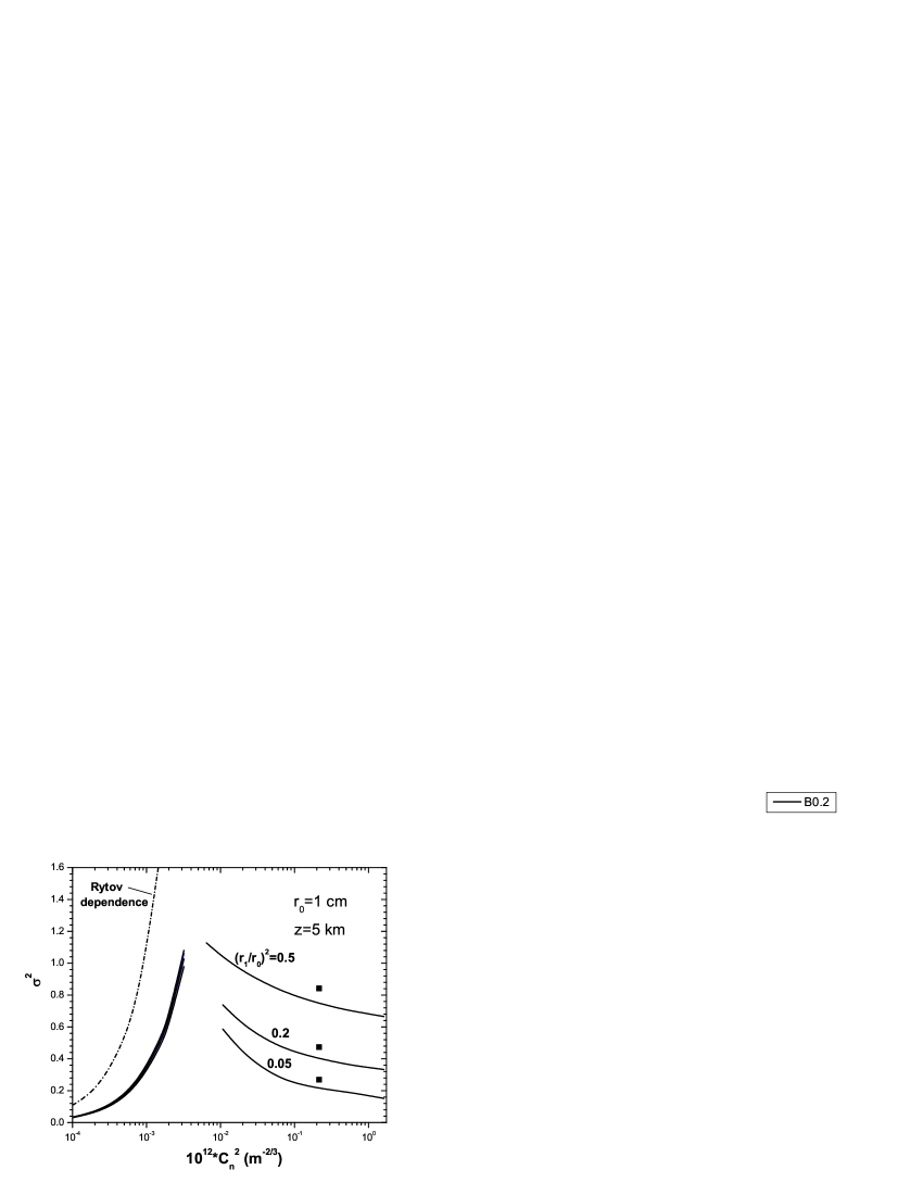
Figure 3: Plots $\sigma^{2}(C_{n}^{2})$ for different initial coherence $(r_{1}/r_{0})^{2}$; $q_{0}$ and $l_{0}$ are as in Fig. 1. Left-side curves calculated with employing Eqs. (48) and (49) exhibit negligible effect of partial coherence (merged curves), that is in contrast to results shown in Fig. 2. Two very different parameters $\rho_{0}^{2}$ are used in these cases. Black squares show $\sigma^{2}$ obtained with the assumption of straight trajectories in Eq. (36).

There is a very simple physical explanation of the reduction of $\sigma^{2}$. Two things are very important for understanding this phenomenon. First of all, in the course of the irradiance propagation the beam acquires the properties of Gaussian statistics. Therefore, the asymptotic value of the intensity correlations $<I(t)I(t)>$ is given by $2<I>^{2}$. On the other hand, the quadratic detector counts are determined not by simultaneous correlations, but by the average $<I(t)I(t+\tau)>$, where the characteristic value of $\tau$ is of the order of $\tau_{d}$. In the limiting case of $\lambda_{c}\rightarrow 0$ and $\tau>>\tau_{s}$ (slow detector), there are no correlations between $I(t)$ and $I(t+\tau)$. Hence, $<I(t)I(t+\tau)>=<~{}I>^{2}$, and the normalized variance of the intensity fluctuations is negligible ($\sigma^{2}\rightarrow 0$). This physical picture is quite similar to the well-known Hanbary-Braun-Twiss effect [29], or photon bunching for thermal light: at zero delay the correlation function has twice the value for long delays.

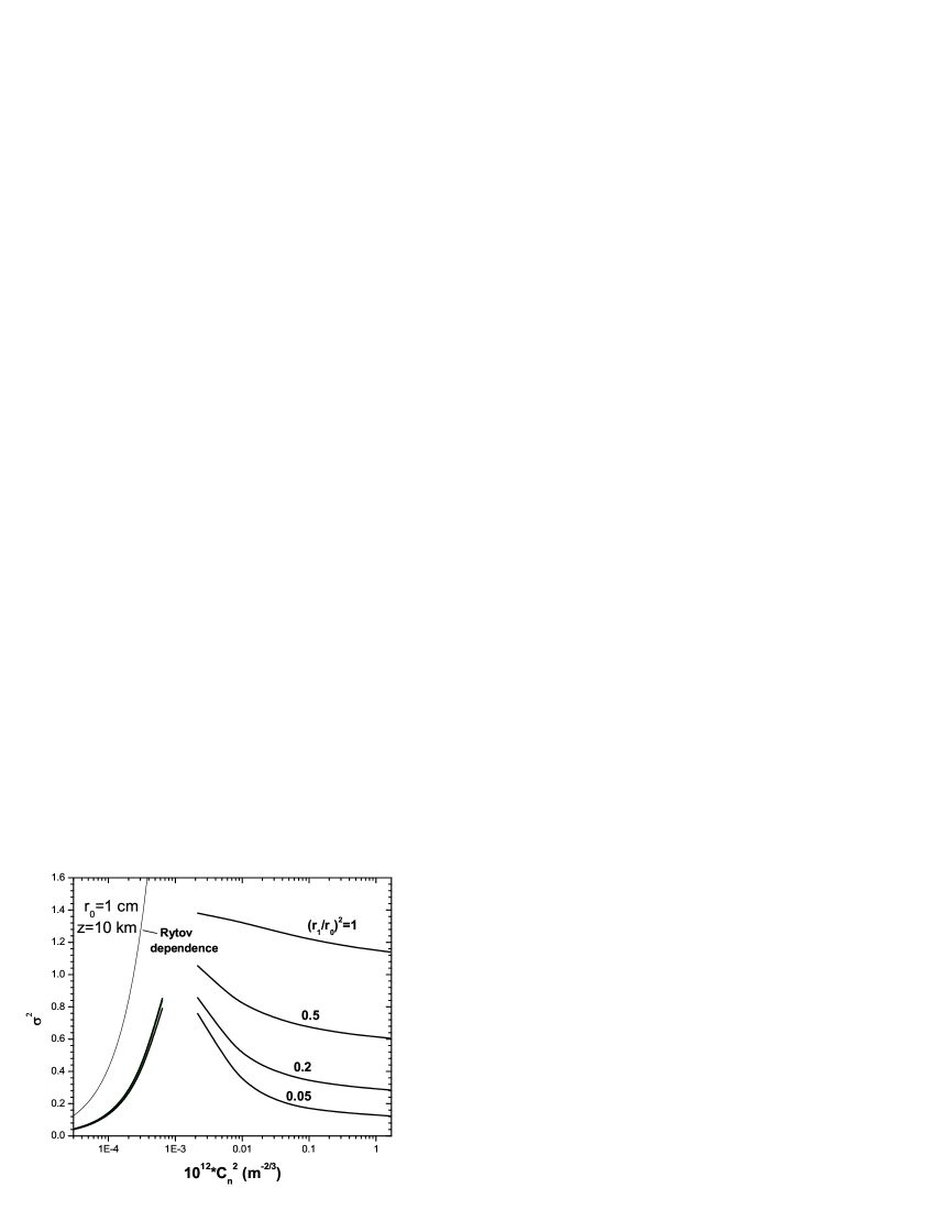
Figure 4: The same as in Fig. 3 but for longer distance. The upper curve corresponds to coherent beam. It approaches asymptotically to value $\sigma^{2}=1$.

For finite values of $\lambda_{c}$, the irradiance differs from thermal light resulting in a finite value of the scintillation index. Our theory gives the scintillation index equal to $r_{1}^{2}/r_{0}^{2}$, that is the relative part of the aperture where the exiting light may be considered as a coherent light.

It should be noted that the finite value of $\sigma^{2}$ shows an absence of full thermalization because the memory of the photon flux about source correlations still exists. This memory may be lost due to fluctuations of the photon transit time $\delta t$. [The transit time was assumed to be constant (equal to $z/c$) in the previous analysis.] When $\delta t\not=0$, the initial conditions for $f({\bf r},{\bf q},t)$ correspond not to its value at the aperture plane, but, for example, to some outlying point $\delta z=c|\delta t|$ where the turbulence has already modified the waves. The estimate of $\delta z$ is given by its rms value. Setting

$$\delta z=\int_{0}^{z}dz^{\prime}\delta n(z^{\prime}),$$

we can easily obtain $<(\delta z)^{2}>\sim 0.066\pi^{2}zC_{n}^{2}L_{0}^{5/3}$. When $C_{n}^{2}=10^{-13}m^{-2/3}$, $L_{0}=10m,z=10^{5}m$, we have $<(\delta z)^{2}>^{1/2}\sim 0.55*10^{-3}m$ and $|\delta t|\sim 2*10^{-12}s$, which is negligibly small.

Other causes of transit time fluctuations arise from fluctuations of the transverse velocity of the photons. For nonzero $q_{\bot}$ the photon velocity in the $z$ direction is given by

$$c_{z}=\frac{\partial\omega_{\bf q}}{\partial q_{z}}\approx c\Bigg{(}1-\frac{q_{\bot}^{2}}{2q_{0}^{2}}\Bigg{)}.$$ (50)

Assuming $q_{\bot}$ to be caused by the turbulence, we have

$${\bf q}(z)=\int_{0}^{z}{\bf F}(z^{\prime})dz^{\prime}/c,$$ (51)

where indices _⊥ are omitted again. Then, using Eqs. (50) and (51) we may estimate $\delta t$ as

$$\delta t\sim\int_{0}^{z}\frac{dz^{\prime}}{c}\Bigg{<}\frac{1}{1-q^{2}/2q_{0}^{2}}-1\Bigg{>}\approx\int_{0}^{z}\frac{dz^{\prime}}{c}\frac{<q^{2}(z^{\prime})>}{2q_{0}^{2}}\approx 1.7\frac{z^{2}C_{n}^{2}}{cl_{0}^{1/3}}.$$ (52)

For the same parameters used previously, $\delta t\sim 3*10^{-11}s$ and $<(\delta z)^{2}>^{1/2}\approx 9*10^{-3}m$, which is negligible again.

The most serious assumption of our approach is that the influence of the turbulence on the photon distribution can be described in terms of a random force ${\bf F}({\bf r})$ (see Eq. (7)) modifying photon momentum ${\bf q}\bot z$. Mathematically, this approximation can be justified when the width of the photon distribution in momentum space is greater than those turbulence wave vectors, which give the dominant contribution to $\sigma^{2}$. In the vicinity of the source, the photon momentum is distributed within the range of the order of $\pi/r_{1}$. (See Eq. (23).) The turbulence spectrum covers very broad interval of wave vectors $[\pi/L_{0},\pi/l_{0}]$ where $L_{0}/l_{0}\sim 10^{5}$. Therefore, it is not clear a priori what wave vector should be taken for the comparison. Of course, the condition $r_{1}\leq l_{0}$ is sufficient to validate our approach. At the same time, this condition imposes very rigid restriction on real optical systems. Fortunately, it is not obligatory for a reliable solution for long-distance propagation. Fist of all, it may be assumed that a broad range of the turbulence spectrum, rather than wave vectors equal to $\pi/l_{0}$, contributes significantly to measured quantities. If this is true, these quantities would not be sensitive to the boundary values of wave vectors. In this context, it is important to note that the beam radius really does exhibit a weak dependence on $l_{0}$. [It depends on $l_{0}$ through $T\sim l_{0}^{-1/3}$, see Eq. (26).] Hence, it is reasonable to consider the characteristic value of the turbulence wave vector to be much smaller than $\pi/l_{0}$.

On the other hand, due to the action of the random force, there is a diffusion-like increase in the transverse momentum of photons in the course of their propagation. It is just that quantity (not $\pi/r_{1}$) which should be compared with the turbulence wave vectors for large $z$. Using Eq. (51) we may estimate the increase of the transverse momentum as

$$<q^{2}>=0.066{\pi}^{2}\Gamma\Bigg{(}\frac{1}{6}\Bigg{)}q_{0}^{2}zC_{n}^{2}(2\pi/l_{0})^{1/3}.$$ (53)

Substituting the previous parameters into Eq. (53), we get $<q^{2}>/{\pi}^{2}l_{0}^{-2}\approx 10^{2}$. This estimate shows our approach to be reliable for long distance propagation. At small distances, the perturbation theory is applicable.

7 Conclusion

The approach presented in this paper can be used for both stationary beams as well as for beams with varying intensity. Also, the statistics of the exiting irradiance may differ from the statistics of coherent or partially coherent beams. Our method of obtaining the correlation function for the intensity fluctuations is not based on the solution of an equation for the fourth-order correlation function. Moreover, we have obtained the asymptotic value for all moments of the intensity fluctuations. Our method does not employ Markov approximation used previously to derive the equation for the fourth-order correlation function. Also, we do not use the so-called quadratic approximation, which like the Markov approximation is nothing more than an artificial modification of the refractive index covariance in order to simplify the theoretical treatment. Both simplifications are inherent to papers [18] and [19]. Besides that, there was assumed $l_{0}=0$, that is impossible within our consideration. Suffice it to say that in the case of $l_{0}=0$, the quantities $T$ and $\gamma$ lose their physical sense because of infinitely large values. In spite of the presence of so serious approximations, the asymptotic ($z\rightarrow\infty$ or $C_{n}^{2}\rightarrow\infty$) results of [18] and our paper results are very similar. The explanation of this follows from the result obtained: the asymptotic value of $\sigma^{2}$ does not depend on the atmosphere turbulence mechanism. Therefore, it does not matter what kind of turbulence spectrum is employed in the case of saturated fluctuations. At the same time, our calculations show (see Figs. 3 and 4) that the distinct asymptotic regime scarcely can be reached in real experiments. Thus, for practice, it is more important to know the behavior of $\sigma^{2}$ at large but finite $C_{n}^{2}$ and $z$ than its asymptotic value. In this case, the real turbulence spectrum as well as an adequate theoretical analysis are required. In this context, the motivations of our studies are evident.

Our calculations show how to suppress the intensity fluctuations using a PCB. The conditions required for this are a random phase modulation of the signal and the use of a slow detector. Estimations of the utility of the PCB should take into account the negative factor of worsening for the receiving system resolution when $\tau_{d}$ is increased. Also, it is important for the experiment performance, that the ratio $\tau_{s}/\tau_{d}$ is always finite, and just this ratio rather than $(r_{1}/r_{0})^{2}$ determines the asymptotic value of $\sigma$ when $(\tau_{s}/\tau_{d})>(r_{1}/r_{0})^{2}$. Hence, the regime of fast phase modulations (but not the increase of $\tau_{d}$) is preferable in both cases.

8 Acknowledgment

We are grateful to V.N. Gorshkov for helping us with illustrative material, and to L.C. Andrews and B.M. Chernobrod for useful discussions. This work was supported by the Department of Energy (DOE) under Contract No. W-7405-ENG-36.

References

- [1] V.I. Tatarskii, The Effects of the Turbulent Atmosphere on Wave Propagation (National Technical Information Service, U.S. Dept. of Commerce, Springfield, Va., 1971).
- [2] L.C. Andrews and R.L. Phillips, Laser Beam propagation through Random Media, SPIE Press, Bellingham, WA (1998).
- [3] L.C. Andrews, R.L. Phillips, and C.Y.Hopen, Laser Beam Scintillation with Applications, SPIE Press, Bellingham, WA (2001).
- [4] R.L. Fante, Proc. IEEE, 63, 1669 (1975).
- [5] R.L. Fante, Proc. IEEE, 68, 1424 (1980).
- [6] I.G. Yakushkin, Izv. VUZ Radiofiz. 28 795 (1985)(Radiophys. Quantum Electron. 28)
- [7] Yu.A. Kravtsov, Rep. Prog. Phys., 39, (1992).
- [8] R.L. Fante, J. Opt. Soc. Am., 69, 71 (1979).
- [9] V.I. Polejaev and J.C. Ricklin, ”Controlled phase diffuser for a laser communication link,” in Artificial Turbulence for Imaging and Wave Propagation, SPIE, 3432, 103 (1998).
- [10] J.C. Ricklin and F.M. Davidson, J. Opt. Soc. Am. A 19 1794 (2002).
- [11] A. Dogariu and S. Amarande, Opt. Lett. 28, 10 (2003).
- [12] G. Gbur and E. Wolf, Opt.Comm., 199, 295 (2001).
- [13] G. Gbur and E. Wolf, J. Opt. Soc. Am. A, 19, 1592 (2002)
- [14] M. Salem, T. Shirai, A. Dogariu, and E. Wolf, Opt. Comm., 216, 261 (2003)
- [15] J.C. Ricklin and F.M. Davidson, SPIE 4885 (2002).
- [16] Y. Baykal, M.A. Plonus, and S.J. Wang, Radio. Sci. 18, 551 (1983).
- [17] Y. Baykal and M.A. Plonus, J. Opt. Soc. Am. A 2, 2124 (1985).
- [18] V.A. Banakh, V.M. Buldakov, and V.L. Mironov, Opt. Spectrosk., 54, 1054 (1983).
- [19] V.A. Banakh and V.M. Buldakov, , Opt. Spectrosk., 55, 707 (1983).
- [20] O. Korotkova, L.C. Andrews, and R.L. Phillips, Proc. SPIE, 4821, 98 (2002).
- [21] O. Korotkova, L.C. Andrews, and R.L. Phillips, Opt. Eng., 43, 330 (2004).
- [22] I.G. Yakushkin, Izv. Vyssh. Uchebn. Zaved., Radiofyz., 18, 1660 (1975).
- [23] R. Dashen, J. Math. Phys., 20, 894 (1979).
- [24] R.L. Fante, Radio Sci., 15, 757 (1980).
- [25] L.D. Landau and E.M. Lifshitz, Electrodynamics of Continuous Media (Pergamon, London 1960)
- [26] J. Strohbehn and S. Clifford, IEEE Trans. Antennas. Propagat., AP-15, 416 (1967).
- [27] E. Collett and R. Alferness, J. Opt. Soc. Amer., 62, 529 (1972).
- [28] P.M. Tomchuk and A.A. Chumak, Sov. Solid State Physics, 15, 1011 (1973).
- [29] L. Mandel and E.Wolf, Optical coherence and quantum optics, Cambridge University, Cambridge, 1995.
- [30] L. Mandel, Phys. Rev. 144, 1071 (1966).