Unitary invariants of qubit systems

Abstract

We give an algorithm allowing to construct bases of local unitary invariants of pure $k$-qubit states from the knowledge of polynomial covariants of the group of invertible local filtering operations. The simplest invariants obtained in this way are explicited and compared to various known entanglement measures. Complete sets of generators are obtained for up to four qubits, and the structure of the invariant algebras is discussed in detail.

1 Introduction

From a mathematical point of view, Quantum Information Theory deals with finite dimensional Hilbert spaces, the state spaces of finite $k$-partite systems, which have the special form

$${\cal H}=V_{1}\otimes V_{2}\otimes\cdots\otimes V_{k}\,,$$ (1)

where $V_{i}$ is the finite dimensional state space of the $i$th part (or particle) of the system, most of the time assumed to be a qubit, which means that $\dim\,V_{i}=2$.

The interesting non-classical behaviors on which the theory is based already occur for two-qubit systems, for the so-called entangled states, those $\psi\in V_{1}\otimes V_{2}$ which cannot be written in the form $v_{1}\otimes v_{2}$. The properties of such states are the basis of the EPR paradox [Einstein et al. 1935], and since its discovery, the entanglement phenomenon has been thoroughly investigated by physicists, cf. [Bell 1966, Clauser et al. 1969, Aspect et al. 1982, Bennett and Wiesner 1992], and more recently by mathematicians, e.g., [Brylinski and Brylinsky 2002, Klyachko 2002, Meyer and Wallach 2002].

There is, however, no general agreement on the definition of entanglement for systems with more than two parts. Klyachko has proposed [Klyachko 2002, Klyachko and Shumovsky 2003] to regard as entangled the states which are semi-stable for the action of the group of invertible local filtering operations, also called SLOCC,

$$G=SL(V_{1})\times\cdots\times SL(V_{k})$$ (2)

in the sense of geometric invariant theory, which means those states on which at least one non trivial $G$-invariant polynomial does not vanish. The point of introducing geometric invariant theory is that this theory provides methods for characterizing such states without explicitly computing the invariants. In order to explore the significance of this property, the invariants have been explicited in the simplest cases (up to 4 qubits, and 3 qutrits, with partial results for 5 qubits, [Luque and Thibon 2003, Luque and Thibon 2005, Verstraete et al. 2002]).

One would also like to quantify entanglement. The non-locality properties of an entangled state does not change under unitary operations acting independently on each of its sub-systems. The idea of describing entanglement by means of local unitary invariants is explored in [Grassl et al. 1998], see also [Schlienz and Mahler 1996, Schlienz and Mahler 1995]. However, except for the simplest systems, there are far too many orbits and a complete classification is out of reach.

An intermediate possibility is to look at the $G$-orbits. The knowledge of the $G$-invariant polynomials is not sufficient to separate the $G$-orbits, and in general, one has to look for the covariants in the sense of classical invariant theory.

In [Briand et al. 2003], the algebra of $G$-covariants for $4$ qubits has been investigated, and a complete set of generators has been obtained.

In the present article, we will explain how these results can be applied to the calculation of bases of unitary invariants. As an application, we compute bases of the spaces of local unitary and special unitary invariants of degree $4$ of $k$ qubits for arbitrary $k$, and recover the results of [Grassl et al. 2002] for 3 and 4 qubits.

The paper is organized as follows. In Section 3 we recall some background on SLOCC covariants, and we describe a method allowing to obtain from them local unitary (LUT) and special unitary (LSUT) invariants. Section 4 is devoted to the computation of the simplest LUT and LSUT invariants from SLOCC covariants. Finally, we give some examples and applications in Section 5.

2 Invariants and covariants of qubit systems

2.1 Group actions on state spaces

Let $V={\mathbb{C}\,}^{2}$ be the local Hilbert space of a two-state system (a qubit), and ${\cal H}=V^{\otimes k}$ be the state space of a system of $k$ qubits. We shall regard it as the natural representation of the group $G=G_{{\mbox{\tiny SLOCC}}}=SL(2,{\mathbb{C}\,})^{k}$, known in quantum information theory as the group of reversible local filtering operations, or stochastic local quantum operations assisted by classical communication (SLOCC) [Bennett and Wiesner 1992, Dür et al. 2001]. This is a semisimple complex Lie group, whose representation theory follows immediately from that of $SL(2,{\mathbb{C}\,})$. The maximal compact subgroup of $G$ is $K=G_{{\mbox{\tiny LSUT}}}=SU(2)^{k}$, the group of local special unitary transformations. We shall also be interested in arbitrary local unitary transformations, which form the group $U=G_{{\mbox{\tiny LUT}}}=U(2)^{k}$.

If $|j\rangle$, $j=0,1$ is a basis of $V$, a state $|\Psi\rangle$ can be written as

$$|\Psi\rangle=\sum_{i_{1},\ldots,i_{k}=0}^{1}a_{i_{1}i_{2}\cdots i_{k}}|i_{1}i_{2}\cdots i_{k}\rangle$$ (3)

where, as customary in the physics literature,

$$|i_{1}i_{2}\cdots i_{k}\rangle=|i_{1}\rangle\otimes\cdots\otimes|i_{k}\rangle\,.$$ (4)

It will be convenient to interpret such a state as a multilinear form

$$f({\bf x})=f(x^{(1)},\ldots,x^{(k)})=\sum_{i_{1},\ldots,i_{k}=0}^{1}a_{i_{1}i_{2}\cdots i_{k}}x^{(1)}_{i_{1}}\cdots x^{(k)}_{i_{k}}\,,$$ (5)

where $x^{(j)}=(x^{(j)}_{0},x^{(j)}_{1})$ are pairs of variables.

The action of a $k$-tuple of matrices ${\bf g}=(g^{(1)},\ldots,g^{(k)})$ on the various vector spaces introduced so far is defined by ${\bf g}{\bf x}={\bf x}^{\prime}$, $x^{\prime(i)}=g^{(i)}x^{(i)}$ and the components $a^{\prime}_{i_{1}i_{2}\cdots i_{k}}$ of $f^{\prime}={\bf g}f$ are defined by the condition

$$\sum_{i_{1},\ldots,i_{k}}a_{i_{1}i_{2}\cdots i_{k}}x^{(1)}_{i_{1}}\cdots x^{(k)}_{i_{k}}=\sum_{i_{1},\ldots,i_{k}}a^{\prime}_{i_{1}i_{2}\cdots i_{k}}x^{\prime(1)}_{i_{1}}\cdots x^{\prime(k)}_{i_{k}}\,.$$ (6)

In the following, we shall be interested in LUT and LSUT invariants of a state $|\psi\rangle$, i.e. polynomial functions $I({\bf a},\bar{\bf a})$ in the components of $|\psi\rangle$, such that

$$I({\bf a},\bar{\bf a})=I({\bf a}^{\prime},\bar{\bf a}^{\prime})\,$$ (7)

where $a^{\prime}_{i_{1}\cdots i_{k}}$ are the components of $f^{\prime}={\bf g}f$ for ${\bf g}$ a LUT or a LSUT. Our main point will be the application of the SLOCC invariant theory to the calculation of such unitary invariants.

2.2 SLOCC Invariants

The SLOCC invariants are the holomorphic polynomials $I({\bf a})$ such that $I({\bf a})=I({\bf a}^{\prime})$ for ${\bf g}\in G_{\mbox{\tiny SLOCC}}$. Of course, the squared modulus $|I|^{2}$ of a SLOCC invariant is a LSUT invariant, but only a small subset of unitary invariant are of this form.

The methods of classical invariant theory can be applied to the determination of the SLOCC invariants of $k$ qubits for small $k$. An important preliminary step is the determination of the Hilbert series

$$h(t)=\sum_{d\geq 0}t^{d}\dim S^{d}({\cal H})^{G_{\mbox{\tiny SLOCC}}},$$ (8)

the generating series of the dimension of the space of homogeneous polynomial invariants of degree $d$.

For $k=3$, the only fundamental polynomial invariant of three qubits is known since the nineteenth century, it is the Cayley hyperdeterminant [Le Paige 1881], see also [Miyake 2003]:

$${\bf Det}(A)=(a_{000}^{2}a_{111}^{2}+a_{001}^{2}a_{110}^{2}+a_{010}^{2}a_{101}^{2}+a_{011}^{2}a_{100}^{2})\\ -2(a_{000}a_{001}a_{110}a_{111}+a_{000}a_{010}a_{101}a_{111}+a_{000}a_{011}a_{1000}a_{1111}\\ +a_{001}a_{010}a_{101}a_{110}+a_{001}a_{011}a_{110}a_{100}+a_{010}a_{011}a_{101}a_{100}\\ ++4(a_{000}a_{011}a_{101}a_{110}+a_{001}a_{010}a_{100}a_{111})$$ (9)

The polynomial invariants of four qubits were constructed in [Luque and Thibon 2003]. Here, the Hilbert series is

$$h(t)=\frac{1}{(1-t^{2})(1-t^{4})^{2}(1-t)^{6}}\,.$$ (10)

For five qubits, the Hilbert series and a few fundamental invariants were obtained in [Luque and Thibon 2005].

2.3 Covariants

To construct the invariants, as well as for the more difficult problem of classifying the orbits, one needs of the classical notion of a covariant. A covariant $\Phi$ of $f$ is a multi- homogeneous $G_{\mbox{\tiny SLOCC}}$-invariant polynomial in the form coefficients $a_{i_{1}\ldots i_{k}}$ and in the original variables $x^{(i)}_{j}$, that is, an invariant in some space

$$\Phi\in S^{(d)}({\cal H})\otimes S^{\alpha_{1}}(V^{*})\otimes\cdots\otimes S^{\alpha_{k}}(V^{*})\,,$$ (11)

where $\alpha$ is the multidegree of $\Phi$ in the $x^{(i)}_{j}$.

Clearly, a covariant can be interpreted as an equivariant map $u_{\Phi}$ from the irreducible representation

$$S_{\alpha}(V):=S^{\alpha_{1}}(V)\otimes\cdots\otimes S^{\alpha_{k}}(V)$$ (12)

of $G$ to $S^{d}({\cal H})$. Such a map is uniquely determined by the image of the highest weight vector $v_{\alpha}$ of $S_{\alpha}(V)$. This highest weight vector is the coefficient of the highest monomial in $\Phi$, classically called the source of the covariant. The coefficients of the other monomials form a basis of weight vectors in the image of $u_{\Phi}$.

The covariants form an algebra, which is naturally graded with respect to $d$ and $\alpha$. We denote by ${\cal C}_{d;\alpha}$ the corresponding graded pieces. The knowledge of their dimensions $c_{d;\alpha}$ is equivalent to the decomposition of the character of $S^{d}({\cal H})$ into irreducible characters of $G$, and the knowledge of a basis of ${\cal C}_{d;\alpha}$ allows one to write down a Clebsch-Gordan series with respect to $G$ for any polynomial in ${\bf a}$. Also, it is known that the equations of any $G$-invariant closed subvariety of the projective space ${\mathbb{P}}({\cal H})$ are given by the simultaneous vanishing of the coefficients of some covariants.

A modern introduction to classical invariant theory can be found in the book [Olver 1999].

3 LUT-invariants from SLOCC-covariants

3.1 General construction

A generating set of the algebra of the polynomial covariants for the action of the SLOCC group can be in principle computed by a slight adaptation of the classical method (the Cayley Omega process, see, e.g., [Olver 1999]). The covariants can be obtained recursively from the simplest one (the ground form $f$)

$$f=\sum_{i_{1}\cdots i_{k}}a_{i_{1}\cdots i_{k}}x^{(1)}_{i_{1}}\cdots x^{(k)}_{i_{k}},$$ (13)

by iterating an operation called transvection, defined by

$$\begin{array}[]{ll}(\Psi,\Phi)^{\epsilon_{1}\cdots\epsilon_{k}}=&{\rm tr\,}\Omega_{x^{(1)}}^{\epsilon_{1}}\cdots\Omega_{x^{(k)}}^{\epsilon_{k}}\Psi({x^{\prime}}^{(1)},\cdots,{x^{\prime}}^{(k)})\times\\ &\times\Phi({x^{\prime\prime}}^{(1)},\cdots,{x^{\prime\prime}}^{(k)})\end{array}$$ (14)

where

$$\Omega_{x}=\det\left|\begin{array}[]{cc}\partial\over\partial{x^{\prime}}_{0}&\partial\over\partial{x^{\prime}}_{1}\\ \partial\over\partial{x^{\prime\prime}}_{0}&\partial\over\partial{x^{\prime\prime}}_{1}\end{array}\right|$$ (15)

and ${\rm tr\,}:x^{\prime},x^{\prime\prime}\rightarrow x$.

In practice, obtaining a description of the algebra in terms of generators and syzygies seems to be out of reach for more than four qubits [Briand et al. 2003, Luque and Thibon 2005]. Nevertheless it may be always possible to compute the smallest covariants with relevant geometric properties.

As already mentioned, a basis ${\rm Cov}_{k}$ of the space of the polynomial SLOCC-covariants can be identified with a basis of highest weight vectors in the symmetric algebra $S({\cal H})$, so that one can write

$$S(V^{\otimes k})=\bigoplus_{\phi\in{\rm Cov}_{k}}V_{\phi},$$

where $V_{\phi}$ denotes the irreducible representation of $G$ whose highest weight vector corresponds to the covariant $\phi$.

Polynomial invariants under LUT (resp. LSUT) live in $S(V^{\otimes k})\otimes S(V^{*\otimes k})$ and hence in

$$\displaystyle\bigoplus_{\phi,\phi^{\prime}\in{\rm Cov}_{k}\atop{\rm deg}\phi={\rm deg}\phi^{\prime}}\left(V_{\phi}\otimes V_{\phi^{\prime}}^{*}\right)^{{\mbox{\tiny LUT}}}$$ (16)

$$\displaystyle(\mbox{resp. }\bigoplus_{\phi,\phi^{\prime}\in{\rm Cov}_{k}}\left(V_{\phi}\otimes V_{\phi^{\prime}}^{*}\right)^{{\mbox{\tiny LSUT}}})\,,$$ (17)

where deg$\phi$ denotes the degree of $\phi$ in the variables $a_{i_{1}\dots i_{k}}$.

Note that if $\phi$ is a covariant whose multidegree in the auxiliary variables is $(n_{1},\dots,n_{k})$ the corresponding irreducible representation is

$$V_{\phi}\simeq S^{n_{1}}\left({\mathbb{C}\,}^{2}\right)\otimes\cdots\otimes S^{n_{k}}\left({\mathbb{C}\,}^{2}\right).$$ (18)

If $\phi$ and $\phi^{\prime}$ are two polynomial covariants whose respective multidegrees are $(n_{1},\dots,n_{k})$ and $(m_{1},\dots,m_{k})$, then $V_{\phi}\otimes V_{\phi^{\prime}}^{*}$ contains polynomial invariants under LUT (resp. LSUT) if and only if $n_{1}=m_{1},\cdots,n_{k}=m_{k}$. Moreover, combining the previous abstract nonsense identifying covariants with $G$-highest weight vectors and $G$-equivariant maps, and the canonical antilinear isomorphism of a Hilbert space with its hermitian dual implies the following result:

Proposition 3.1

Denoting by $\Phi_{d,i}^{\alpha}$ a basis of SLOCC covariants of degree $d$ in the entries of the tensor and multidegree $\alpha$ in the auxiliary variables, one has:

1. The scalar products $\langle\Phi_{d,i}^{\alpha}|{{\Phi}_{d,j}^{\alpha}}\rangle$ with respect to the auxiliary variables, the $a_{i_{1}\ldots i_{k}}$ being regarded as scalars, form a basis of the space of LUT invariants.

2. Similarly, the scalar products $\langle\Phi_{d,i}^{\alpha}|{{\Phi}_{d^{\prime},i}^{\alpha}}\rangle$ (where $d^{\prime}$ is not necessarily equal to $d$), form a basis of the space of LSUT invariants.

The hermitian scalar product induced by the one of $V$ can be calculated by the formula

$$\langle x_{1}\cdots x_{m}|y_{1}\cdots y_{m}\rangle={\rm perm}\left(\langle x_{i}|y_{j}\rangle\right)$$

if $\langle x_{i}|y_{j}\rangle=1$ when $x_{i}=y_{j}$ and $0$ otherwise.

This property should be of interest for the study of entanglement measures, which are special LSUT invariants. Indeed, expressing such a measure as a simple combination of scalar products of covariants with known geometric properties might lead to interesting insights.

In the sequel, we will denote by ${\rm Cov}_{{\mbox{\tiny SLOCC}}}(k)$ (resp. ${\rm Inv}_{{\mbox{\tiny LUT}}}$, ${\rm Inv}_{{\mbox{\tiny LSUT}}}$) the algebra of polynomial SLOCC-covariants (resp. LUT-invariants, LSUT-invariants). Note that these algebras are multigraded. The space of multihomogeneous SLOCC-covariants (resp. LUT-invariants, LSUT -invariants) of degree $n$ in the $a_{i_{1}\cdots i_{k}}$ and ${\bf d}=(d_{1},\cdots,d_{k})$ in the auxiliary variables (resp. degree $n$ in the $a_{i_{1}\cdots i_{k}}$’s and the $\overline{a}_{i_{1}\cdots i_{k}}$’s, degree $n_{1}$ in the $a_{i_{1}\cdots i_{k}}$’s and degree $n_{2}$ the $\overline{a}_{i_{1}\cdots i_{k}}$’s) will be denoted by ${\rm Cov}_{{\mbox{\tiny SLOCC}}}(k;n;{\bf d})$ (resp. ${\rm Inv}_{{\mbox{\tiny LUT}}}(k;n)$, ${\rm Inv}_{{\mbox{\tiny LSUT}}}(k;(n_{1},n_{2}))$).

3.2 Hilbert series

From Proposition 3.1, we see that the knowledge of the Hilbert series of the SLOCC-convariants allows one to compute the Hilbert series of the LUT and LSUT-invariants. We will denote by

$${h}_{{\mbox{\tiny SLOCC}}}(k;z;{\bf u})=\sum\dim{\rm Cov}_{{\mbox{\tiny SLOCC}}}(n;k;{\bf d})z^{n}{\bf u}^{\bf d}$$ (19)

where ${\bf u}^{\bf d}=u_{1}^{d_{1}}\cdots u_{k}^{d_{k}}$, the Hilbert series of ${\rm Inv}_{{\mbox{\tiny SLOCC}}}$. The Hilbert series of the algebras ${\rm Inv}_{{\mbox{\tiny LUT}}}$ and ${\rm Inv}_{{\mbox{\tiny LSUT}}}$ are obtained from ${h}_{{\mbox{\tiny SLOCC}}}(k;z;{\bf u})$ by the formulae

$$\begin{array}[]{rcl}{h}_{{\mbox{\tiny LUT}}}(k;z)&=&\sum_{n}\dim{\rm Inv}_{{\mbox{\tiny LUT}}}(k;2n)z^{2n}\\ &=&\left.{h}_{{\mbox{\tiny SLOCC}}}(k;z^{2};{\bf u})\odot{h}_{{\mbox{\tiny SLOCC}}}(k;z^{2};{\bf u})\right|_{u_{i}=1}\\ &=&{\rm CT}_{z,u_{1},\dots,u_{k}}\left\{{h}_{{\mbox{\tiny SLOCC}}}(k;zt;(u_{1},\dots,u_{k})){h}_{{\mbox{\tiny SLOCC}}}(k;{z\over t};(u_{1}^{-1},\dots,u_{k}^{-1})\right\}\,,\end{array}$$ (20)

where $\odot$ denotes the Hadamard product of the power series ring ${\mathbb{C}\,}[[z,u_{1},\dots,u_{k}]]$ (that is, ${\bf u}^{\alpha}\odot{\bf u}^{\beta}=\delta_{\alpha\beta}{\bf u}^{\alpha}$), and ${\rm CT}_{x_{1},\dots,x_{n}}f$ means the constant term of the series $f$ with respect to the variables $x_{1},\dots,x_{n}$.

Similarly, one has

$$\begin{array}[]{rcl}{h}_{{\mbox{\tiny LSUT}}}(k;z)&=&\sum_{n_{1},n_{2}}\dim{\rm Inv}_{{\mbox{\tiny LUT}}}(k;(n_{1},n_{2}))z^{n_{1}}\overline{z}^{n_{2}}\\ &=&\left.{h}_{{\mbox{\tiny SLOCC}}}(k;z;{\bf u})\odot_{{\mathbb{C}\,}[[z,\overline{z}]]}{h}_{{\mbox{\tiny SLOCC}}}(k;\overline{z};{\bf u})\right|_{u_{i}=1}\\ &=&{\rm CT}_{u_{1},\dots,u_{k}}\left\{{h}_{{\mbox{\tiny SLOCC}}}(k;z;(u_{1},\cdots,u_{k}){h}_{{\mbox{\tiny SLOCC}}}(k;\overline{z};(u_{1}^{-1},\cdots,u_{k}^{-1})\right\}\,,\end{array}$$ (21)

where $\odot_{{\mathbb{C}\,}[[z,\overline{z}]]}$ denotes the Hadamard product in ${\mathbb{C}\,}[[z,\overline{z}]][[u_{1},\cdots,u_{k}]]$ (i.e. considering ${\mathbb{C}\,}[[z,\overline{z}]]$ as the ring of scalars).

Hence,

$$\dim{\rm Inv}_{{\mbox{\tiny LUT}}}(k;2n)=\sum_{\bf d}(\dim{\rm Cov}_{{\mbox{\tiny SLOCC}}}(n;k;{\bf d}))^{2}$$ (22)

and

$$\dim{\rm Inv}_{{\mbox{\tiny LSUT}}}(k;(n_{1},n_{2}))=\sum_{{\bf d}}\dim{\rm Cov}_{{\mbox{\tiny SLOCC}}}(n_{1};k;{\bf d})\dim{\rm Cov}_{{\mbox{\tiny SLOCC}}}(n_{2};k;{\bf d}).$$ (23)

Classical methods of invariant theory allows one to express the Hilbert series of algebras of covariants as a constant term (see [Briand et al. 2003] for an example). Hence, the Hilbert series of unitary and special unitary invariants are

$${h}_{{\mbox{\tiny LUT}}}(k;z)=\frac{1}{2^{k}}{\rm CT}_{t,\bf u}\left\{{\displaystyle\prod_{i}(1-u_{i}^{-2})^{2}\over\displaystyle\prod_{\alpha\in\{-1,+1\}^{k+1}\atop a=\pm 1}(1-t^{a}z\prod_{i}{\bf u}^{\alpha})}\right\}$$ (24)

and

$${h}_{{\mbox{\tiny LSUT}}}(k;z)=\frac{1}{2^{k}}{\rm CT}_{\bf u}\left\{\displaystyle\prod_{i}(1-u_{i}^{-2})^{2}\over\displaystyle\prod_{\alpha\in\{-1,+1\}^{k}}\left[(1-z{\bf u}^{\alpha})(1-\overline{z}{\bf u}^{\alpha})\right]\right\}.$$ (25)

These expressions have been first derived by Beth et al. (unpublished, see [Grassl et al. 2002]), using a different method.

4 Simplest invariants

4.1 Dimension formulas for SLOCC-covariants

The characters of the irreducible polynomial representations of the group $GL(2,{\mathbb{C}\,})^{k}$ are the products

$$s_{\underline{\lambda}}:=s_{\lambda^{(1)}}\cdots s_{\lambda^{(k)}}$$ (26)

where $\underline{\lambda}=(\lambda^{(1)},\dots,\lambda^{(k)})$ is a tuple of partitions $\lambda^{(i)}$ of length at most 2, and $s_{\lambda^{(i)}}$ the corresponding irreducible character of $GL(2,{\mathbb{C}\,})$ i.e., a Schur function [Macdonald 1991]. In particular, the characters of the one-dimensional representations

$$\det{}^{\bf l}({\bf g})=(\det g^{(1)})^{l_{1}}(\det g^{(2)})^{l_{2}}\cdots(\det g^{(k)})^{l_{k}}\,,$$ (27)

containing the SLOCC invariants, are the products

$$s_{(l_{1}l_{1})}s_{(l_{2}l_{2})}\cdots s_{(l_{k}l_{k})}$$ (28)

and the character of $GL(V)$ in $S^{d}(V)$ is $s_{d}$.

Hence, the dimension of the space of invariants of degree $d$ and weight ${\bf l}$, which is also the multiplicity of the one-dimensional character $\det^{\bf l}$ in $S^{d}(V)$, is given by the scalar product

$$\dim{\rm Inv}_{\mbox{\tiny SLOCC}}(d,k;{\bf l})=\langle s_{d}\,|\,s_{(l_{1}l_{1})}\cdots s_{(l_{k}l_{k})}\rangle$$ (29)

of SLOCC characters (where ${\bf l}=(l_{1},\dots,l_{k})$). We see that ${\rm Inv}_{\mbox{\tiny SLOCC}}(d;k;{\bf l})$ can be nonzero only if the condition

$$d=2l_{1}=2l_{2}=\cdots=2l_{k}$$ (30)

is satisfied. Hence,

$$\dim{\rm Inv}_{\mbox{\tiny SLOCC}}(2l;k)=\sum_{\lambda\vdash 2l\atop l(\lambda)\leq 2}\frac{1}{z_{\lambda}}\chi_{\lambda}^{ll}\cdots\chi_{\lambda}^{ll}\,,$$ (31)

where $\chi_{\lambda}^{ll}$ denotes the value of the irreducible character $\chi^{ll}$ (labelled by the partition $(l,l)$) of the symmetric group ${\mathfrak{S}}_{2l}$ on the conjugacy class $\lambda=(1^{m_{1}}2^{m_{2}}\cdots n^{m_{n}})$, and $z_{\lambda}=\prod_{i}i^{m_{i}}m_{i}!$, cf. [Macdonald 1991].

In the same way, the SLOCC-covariants of a $k$-qubit system form the algebra

$${\rm Cov}=[{S}({V}^{\otimes k})\otimes{S}(V^{*}\oplus\cdots\oplus V^{*})]^{{\mbox{\tiny SLOCC}}}$$ (32)

which can be graded according both to the degree in the $a_{i_{1}\ldots i_{k}}$ and the multidegree in the auxiliary variables. A similar reasoning gives the dimension of the space of covariants of degree $d$ as

$$\dim{\rm Cov}_{\mbox{\tiny SLOCC}}(d;k)=\sum_{\mu\vdash n}\frac{1}{z_{\mu}}\left(\sum_{\lambda\vdash d\atop l(\lambda)\leq 2}\chi_{\mu}^{\lambda}\right)^{k}.$$ (33)

Although impratical for finding closed forms of the Hilbert series, these expressions are useful for computing the first terms.

4.2 Simplest SLOCC-covariants

The space of covariants of degree $1$ is generated by the ground form

$$f=\sum_{0\leq i_{1},\cdots,i_{k}\leq 1}a_{i_{1}\cdots i_{k}}x^{(1)}_{i_{1}}\cdots x^{(k)}_{i_{k}}.$$ (34)

The dimension of the space of covariants of degree 2 of a $k$- qubit system follows from formula (33)

$$\dim{\rm Cov}_{\mbox{\tiny SLOCC}}(2,k)=2^{k-1}.$$ (35)

Observe that the only multihomogeneous covariants in this space have a multidegree in the auxiliary variables belonging to $\{0,2\}^{k}$. If $\bf d$ is any tuple, we will denote by $|{\bf d}|_{a}$ the number of occurrence of $a$ in $\bf d$. The dimension of the space of covariants of degree ${\bf d}=(d_{1},\cdots,d_{k})\in\{0,2\}^{k}$ in the auxiliary variables is

$$\dim{\rm Cov}_{\mbox{\tiny SLOCC}}(2,k;{\bf d})=\langle(\chi^{2})^{(k-|{\bf d}|_{0})}(\chi^{11})^{|{\bf d}|_{0}}|\chi^{2}\rangle=\left\{\begin{array}[]{ll}0&\mbox{if }|{\bf d}|_{0}\mbox{ is odd}\\ 1&\mbox{if }|{\bf d}|_{0}\mbox{ is even}\end{array}\right..$$ (36)

Hence, we can state the following result:

Proposition 4.1

The space of the covariants of degree $2$ of a $k$-qubit system has dimension $2^{k-1}$ and is spanned by $f^{2}$ and the polynomials

$$B_{\bf d}=(f,f)^{{2-d_{1}\over 2},\dots,{2-d_{k}\over 2}}\,,$$ (37)

where ${\bf d}=(d_{1},\cdots,d_{k})\in\{0,2\}^{k}$ and $|{\bf d}|_{0}$ is even.

Note that if $k$ is odd, there are no invariants of degree $2$ and if $k$ is even the invariants are all proportional to the hyperdeterminant $(f,f)^{(1^{k})}$.

The dimension of the space of covariants of degree 3 is, from formula (33),

$$\begin{array}[]{ll}\dim{\rm Cov}_{\mbox{\tiny SLOCC}}(3,k)&=\frac{1}{2}3^{k-1}+\frac{1}{2}.\end{array}$$ (38)

The only covariants of degree $3$ in the entries of the tensor have a multidegree ${\bf d}=(d_{1},\dots,d_{k})\in\{1,3\}^{k}$ in the auxiliary variables. Let ${\bf d}=(d_{1},\dots,d_{k})\in\{1,3\}^{k}$ be a multidegree, the dimension of the space of the covariants having multidegree $\bf d$ is

$$\begin{array}[]{ll}\dim{\rm Cov}_{\mbox{\tiny SLOCC}}(3,k;{\bf d})&=\langle(\chi^{21})^{|{\bf d}|_{1}}(\chi^{3})^{|{\bf d}|_{3}}|(\chi^{3})\rangle\\ &=\frac{1}{3}\left(2^{|{\bf d}|_{1}-1}+(-1)^{|{\bf d}|_{1}}\right)\end{array}$$ (39)

if $|{\bf d}|_{1}>0$, and

$$\dim{\rm Cov}_{\mbox{\tiny SLOCC}}(3,k;(3^{k}))=\langle(\chi^{3})^{k}|\chi^{3}\rangle=1.$$ (40)

This implies that all the homogeneous covariants of multidegree $(3^{n})$ are proportional to $f^{3}$. From (39), the dimension of the space of the $k$-linear covariants of degree $3$ is

$$\begin{array}[]{ll}\dim{\rm Cov}_{\mbox{\tiny SLOCC}}(3,k;{\bf d})&=\frac{1}{3}\left(2^{k-1}+(-1)^{k}\right)\end{array}$$ (41)

Let us denote by $\{C_{i}\}_{i=1,\dots,\frac{1}{3}(2^{k-1}+(-1)^{k-1})}$ a basis of the space of covariants of multidegree $(1^{k})$. Applying transvections with the ground form to the $C_{i}$, we obtain invariants of degree $4$. Remark that the dimension of the space of invariants of degree $4$ is equal to the dimension of the space of multilinear covariants of degree $3$, so that we recover a result of [Brylinski and Brylinsky 2002]. We will denote by $(D_{i})$ a basis of the space of SLOCC invariants of degree $4$.

4.3 Polynomial LUT-invariants of degree $4$

From Proposition 4.1, one can construct a basis of the space of LUT invariants of degree $4$. If ${\bf d}=(d_{1},\dots,d_{k})$, the dimension of ${\rm Cov}_{\mbox{\tiny SLOCC}}(2,k;{\bf d})$ is $0$ or $1$. Hence, the only possibilities are the squared norms

$${\bf B}_{\bf d}:=\langle B_{\bf d}|B_{\bf d}\rangle$$ (42)

where ${\bf d}=(d_{1},\cdots,d_{k})\in\{0,2\}^{k}$ and $|{\bf d}|_{0}$ is even.

The dimension of the space is the coefficient of $z^{4}$ in the Hilbert series

$$\dim{\rm Inv_{{\mbox{\tiny LUT}}}}(4,k)=\sum_{{\bf d}}\left(\dim{\rm Cov}_{\mbox{\tiny SLOCC}}(2,k;{\bf d})\right)^{2}=2^{k-1}.$$ (43)

Thus, the following result holds:

Proposition 4.2

The space of the LUT invariants of degree $4$ of a $k$-qubit system has dimension $2^{k-1}$ and is spanned by the polynomials ${\bf B}_{\bf d}$ and $\langle f|f\rangle^{2}$.

Furthermore, one can show that

$${\bf B}_{22\dots 2}=\langle f^{2}|f^{2}\rangle=2^{k}\langle f|f\rangle^{2}-\sum_{{\bf d}\neq(2,\dots,2)}{\bf B}_{\bf d}\,.$$ (44)

Indeed, $\langle f|f\rangle^{2}=\langle f\otimes f|f\otimes f\rangle$, and the classical Clebsch-Gordan series allows one to express $f\otimes f$ in terms of transvectants, whence the result.

If we consider only the LSUT group, one has generators of bidegree $(4,0)$, $(3,1)$, $(2,2)$, $(1,3)$, $(0,4)$ in the components of the state and their conjugates. The subspace of bidegree $(2,2)$ is the space of LUT-invariants of degree $4$:

$${\rm Inv_{{\mbox{\tiny LSUT}}}}((2,2),k)={\rm Inv_{{\mbox{\tiny LUT}}}}(4,k).$$ (45)

The subspace of bidegree $(4,0)$ if the space of the SLOCC invariants of degree $4$

$${\rm Inv_{{\mbox{\tiny LSUT}}}}((4,0),k)={\rm Inv_{{\mbox{\tiny SLOCC}}}}(4,k).$$ (46)

In the same way, the subspace of bidegree $(0,4)$ is the space of the conjugates of the SLOCC invariants of degree $4$. A basis of the space of the LSUT-invariants of bidegree $(3,1)$ can be obtained from the scalar products $\langle C_{i}|f\rangle$.

Proposition 4.3

The subspace of LSUT-invariants of degree $4$ of a $k$-qubit system has dimension

$$\frac{7}{3}2^{k-1}-\frac{4}{3}(-1)^{k-1}$$

and is spanned by the polynomials $D_{i}$ (bidegree $(4,0)$), ${\bf C}_{i}=\langle C_{i}|f\rangle$ (bidegree $(3,1)$), ${\bf B}_{\bf d}$ (bidegree $(2,2)$), $\overline{\bf C}_{i}$ (bidegree $(1,3)$) and $\overline{D}_{i}$ (bidegree $(0,4)$).

5 Examples

5.1 LUT-invariants and linear entropies

Let $|\Psi\rangle=\sum a_{i_{1}\dots i_{k}}|i_{1}\cdots i_{k}\rangle$ be a pure $k$-qubit state. Meyer and Wallach [Meyer and Wallach 2002] have defined an entanglement measure $\cal Q$ by

$${\cal Q}(|\Psi\rangle)=\frac{1}{k}\sum_{i=1}^{k}D_{1}^{(i)}(|\Psi\rangle)$$ (47)

where

$$D_{1}^{(i)}(|\Psi\rangle)=2\sum_{(\epsilon_{1},\cdots,\epsilon_{k-1})\neq(\epsilon^{\prime}_{1},\cdots,\epsilon^{\prime}_{k-1})}\left|\left|\begin{array}[]{cc}\left(\epsilon_{i}^{0}|\Psi\right)&\left({\epsilon^{\prime}}_{i}^{0}|\Psi\right)\\ \left(\epsilon_{i}^{1}|\Psi\right)&\left({\epsilon^{\prime}}_{i}^{1}|\Psi\right)\end{array}\right|\right|^{2}\,.$$

In this expression, $\left(\epsilon_{i}^{\delta}|\Psi\right)$ denotes the coefficient of $\left|\epsilon_{1}\cdots\epsilon_{i-1}\delta\epsilon_{i+1}\cdots\epsilon_{k}\right\rangle$ in $|\Psi\rangle$, and the double bars mean the squared modulus of the determinant.

The interest of this measure resides in its physical interpretation, related to the average purity of the constituent qubits [Brennen 2003] or the linearised form of the Von Neumann entropy of a single qubit with the rest of the system.

Emary has remarked [Emary 2004] that the functions $D_{1}^{(i)}$ are entanglement monotones, thus in particular LU-invariants. Hence, each $D_{1}^{(i)}$ can be written in terms of squares of transvectants. We have

$$D_{1}^{(i)}=\frac{1}{2^{k-2}}\sum_{d=(d_{1},\cdots,d_{k})\in\{0,2\}^{k}\atop d_{i}=0}{\bf B}_{d}.$$ (48)

Indeed, $D_{1}^{(i)}=\|\Phi_{i}\otimes\Phi_{i}\|^{2}$, where $\Phi_{i}=B_{22\cdots 202\cdots 2}$, and the result follows again from the Clebsch-Gordan series.

Hence, in terms of our basis, the quantity ${\cal Q}(|\Psi\rangle)$ has the simple expression

$${\cal Q}(|\Psi\rangle)=\frac{1}{2^{k-2}k}\sum_{{\bf d}=(d_{1},\cdots,d_{k})\in\{0,2\}^{k}}|{\bf d}|_{0}{\bf B}_{d}.$$ (49)

5.2 LUT-invariants for $3$-qubits

The algebra of covariants of $3$ qubits is generated by the polynomials [Le Paige 1881]

$$f:=\sum a_{i_{1}i_{2}i_{3}}x_{i_{1}}y_{i_{2}}z_{i3}$$

$$H_{x}:=\left|\begin{array}[]{cc}{\partial^{2}f\over\partial y_{0}\partial z_{0}}&{\partial^{2}f\over\partial y_{1}\partial z_{0}}\\ {\partial^{2}f\over\partial y_{0}\partial z_{1}}&{\partial^{2}f\over\partial y_{1}\partial z_{1}}\end{array}\right|$$ (52)

$$H_{y}:=\left|\begin{array}[]{cc}{\partial^{2}f\over\partial x_{0}\partial z_{0}}&{\partial^{2}f\over\partial x_{1}\partial z_{0}}\\ {\partial^{2}f\over\partial x_{0}\partial z_{1}}&{\partial^{2}f\over\partial x_{1}\partial z_{1}}\end{array}\right|$$ (55)

$$H_{z}:=\left|\begin{array}[]{cc}{\partial^{2}f\over\partial x_{0}\partial y_{0}}&{\partial^{2}f\over\partial x_{1}\partial y_{0}}\\ {\partial^{2}f\over\partial x_{0}\partial y_{1}}&{\partial^{2}f\over\partial x_{1}\partial y_{1}}\end{array}\right|$$ (58)

$$T:=\left|\begin{array}[]{cc}{\partial f\over\partial x_{0}}&{\partial f\over\partial x_{1}}\\ {\partial H_{x}\over\partial x_{0}}&{\partial H_{x}\over\partial x_{1}}\end{array}\right|$$ (61)

$$\Delta:=(T,f)^{111}$$

From these polynomials, we can construct the following LU-invariants

$${\bf A}_{111}:=\langle f|f\rangle$$

$${\bf B}_{200}:=\langle H_{x}|H_{x}\rangle$$

$${\bf B}_{020}:=\langle H_{y}|H_{y}\rangle$$

$${\bf B}_{002}:=\langle H_{z}|H_{z}\rangle$$

$${\bf C}_{111}:=\langle T|T\rangle$$

$${\bf D}_{000}:=\langle\Delta|\Delta\rangle$$

$${\bf F}_{222}:=\langle\Delta f^{2}|{T}^{2}\rangle$$

Grassl et al. [Grassl et al. 2002] have computed a minimal system of seven generators (denoted by $f_{i}$) of the algebra of LU invariants. We shall give their expressions in terms of scalar products of covariants.

The generator of degree $2$, $f_{1}$ is clearly ${\bf A}_{111}$. To define generators of degree $4$ and $6$, the authors introduce the notation

$$f_{\sigma,\tau,\rho}:=\sum_{{{\bf i}=(i_{1},i_{2},\dots,i_{n}),\atop{\bf j}=(j_{1},j_{2},\dots,j_{n}),}\atop{\bf k}=(k_{1},k_{2},\dots,k_{n})}{\bf a}_{\bf ijk}{\bf\overline{a}}_{{\bf i}^{\sigma}{\bf j}^{\tau}{\bf k}^{\rho}}$$ (62)

where ${\bf i}^{\sigma}=(i_{\sigma(1)},\dots,i_{\sigma(n)})$ and ${\bf a}_{\bf ijk}=a_{i_{1}j_{1}k_{1}}\cdots a_{i_{n}j_{n}k_{n}}$. Their generators in degree $4$ and $6$ are

$$f_{2}:=f_{(12),(12),{\rm Id}}={\bf A}_{111}^{2}-{\bf B}_{200}-{\bf B}_{020}$$

$$f_{3}:=f_{(12),{\rm Id},(12)}={\bf A}_{111}^{2}-{\bf B}_{200}-{\bf B}_{002}$$

$$f_{4}:=f_{{\rm Id},(12),(12)}={\bf A}_{111}^{2}-{\bf B}_{020}-{\bf B}_{002}$$

$$f_{5}:=f_{(12),(23),(13)}={\bf A}_{111}^{3}+\frac{3}{2}{\bf C}_{111}-\frac{3}{2}{\bf A}_{111}({\bf B}_{200}$$

$$+{\bf B}_{020}+{\bf B}_{002})$$

Note that these invariants appear in many places in the literature, for example in [Kempe 1999].

The generator of degree $8$ is ${\bf D}_{000}$ and the generator of degree $12$ is

$$f_{7}:= \overline{\Delta}\left([11,00]\{00,00\}-[11,00]\{11,11\}\right.$$

$$+[11,01]\{00,01\}+[11,10]\{00,10\}$$

$$+2[11,10]\{01,11\}-2[01,00]\{10,00\}$$

$$-[01,00]\{11,01\}-[10,00]\{11,10\}$$

$$-[10,01]\{00,00\}-[10,01]\{01,01\}$$

$$+[10,01]\{10,10\}\left.+[10,01]\{11,11\}\right)^{2}$$

where $[i_{1}i_{2},j_{1}j_{2}]=a_{i_{1}i_{2}0}a_{j_{1}j_{2}1}-a_{i_{1}i_{2}1}a_{j_{1}j_{2}0}$ and $\{i_{1}i_{2},j_{1}j_{2}\}=a_{i_{1}i_{2}0}\overline{a_{j_{1}j_{2}1}}+a_{i_{1}i_{2}1}\overline{a_{j_{1}j_{2}0}}$. With our notations, one has

$$f_{7}=\frac{1}{2}{\bf D}_{000}\left(\frac{3}{2}\left({\bf B}_{200}+{\bf B}_{020}+{\bf B}_{002}\right)-{\bf A}_{111}^{2}\right)$$

$$+2{\bf C}_{111}^{2}-4{\bf B}_{200}{\bf B}_{020}{\bf B}_{002}+\frac{1}{8}{\bf F}_{222}.$$

The authors of [Grassl et al. 2002] obtained the Hilbert series using residue calculations in Magma. We have been able to reproduce their results evaluating (24) using a very efficient algorithm due to Guoce Xin [Xin 2004] in a Maple implementation. Summarizing, we have:

Proposition 5.1

The algebra of local unitary invariants pure $3$-qubit states is generated by ${\bf A}_{111}$, ${\bf B}_{200}$, ${\bf B}_{020}$, ${\bf B}_{002}$, ${\bf C}_{111}$, ${\bf D}_{000}$ and ${\bf F}_{222}$. Its Hilbert series is

$${h}_{\mbox{\tiny LUT}}(3;z)={1-t^{24}\over(1-t^{2})(1-t^{4})^{3}(1-t^{6})(1-t^{8})(1-t^{12})}$$ (63)

which where the numerator reflects the existence of a unique syzygy in degree $24$.

5.3 Classification of the orbits under SLOCC transformations

The normal forms of $3$-qubit states under SLOCC transformations are known since 1881 [Le Paige 1881]. As shown on table 1, the SLOCC orbits can be characterized by the vanishing or non vanishing of a set of four LU-invariants.

$$\begin{array}[]{ccccc}\hline\cr&{\bf B}_{200}&{\bf B}_{020}&{\bf B}_{002}&{\bf D}_{000}\\ \hline\cr|GHZ\rangle&\times&\times&\times&\times\\ |W\rangle&\times&\times&\times&0\\ |B_{1}\rangle=|001\rangle+|010\rangle&\times&0&0&0\\ |B_{2}\rangle=|001\rangle+|100\rangle&0&\times&0&0\\ |B_{3}\rangle=|010\rangle+|100\rangle&0&0&\times&0\\ |000\rangle&0&0&0&0\\ \hline\cr\end{array}$$

Table 1: SLOCC orbits of three qubit states.

In the table, a $\times$ means the non-nullity of the invariant. Hence, (48) implies that in this case, the “onion classification” [Miyake 2003] can be described only in terms of proper entanglement measures (entanglement monotones), see fig 1.

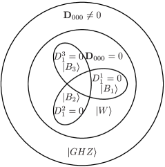
Figure 1: SLOCC orbit structure for $3$-qubits

5.4 LSUT-invariants for $3$-qubits

Another unpublished result of Grassl et al. [Grassl et al. 2002] can be recovered from (25) by means of Xin’s algorithm [Xin 2004]. It is the Hilbert series of the algebra of LSUT-invariants of three qubits,

$${z^{5}\overline{z}^{5}+z^{3}\overline{z}^{3}+z^{2}\overline{z}^{2}+1\over(1-z\overline{z})(1-z^{4})(1-z^{2}\overline{z}^{2})^{2}(1-\overline{z}^{4})(1-z\overline{z^{3}})(1-z^{3}\overline{z})}$$ (64)

This expression suggests that the algebra has a Cohen-Macaulay structure with $6$ primary invariants of respective bidegrees ($(1,1),(0,4),(2,2),(2,2),(4,0),(1,3)$ and $(3,1)$ and $3$ secondary invariants of bidegree $(2,2),(3,3),(5,5)$. The set of primary invariants is

$${\cal P}=\{{\bf A}_{111},f_{2},f_{3},\Delta,\overline{\Delta},s_{2}:=\langle A,T\rangle,\overline{s_{2}}\}\,.$$

Computing the Jacobian of ${\bf A}_{111},f_{2},f_{3},\Delta,\overline{\Delta},s_{2},\overline{s_{2}},a_{000},\dots,a_{111},\overline{a_{000}}$ with the random numerical values given in table 2, one finds

$$-53279560564736-243669580382208i\neq 0.$$

This implies that the polynomials ${\bf A}_{111},f_{2},f_{3},\Delta,\overline{\Delta},s_{2}$ and $\overline{s_{2}}$ are algebraically independent.

$$\begin{array}[]{|c|c|c|c|c|c|c|c|}\hline\cr a_{000}&a_{001}&a_{010}&a_{011}&a_{100}&a_{101}&a_{110}&a_{111}\\ \hline\cr 3+3i&3+3i&3+3i&2+i&3+2i&1+2i&2+3i&3+i\\ \hline\cr\end{array}$$

Table 2: Random values of the $a_{ijk}$’s.

The set of secondary invariants is ${\cal S}=\{f_{4},f_{5},f_{4}f_{5}\}$. The polynomial $f_{4}$ (resp. $f_{5}$) is linearly independent of all algebraic combinations of bidegree $(2,2)$ (resp. $(3,3)$) of elements of $\cal P$. Furthermore, one has two syzygies involving respectively $f_{4}^{2}$ and $f_{5}^{2}$:

$$8f_{1}f_{5}-6f_{4}f_{2}+3f_{4}^{2}-3|\Delta|^{2}+3f_{2}^{2}-6f_{4}f_{3}+f_{1}^{4}+3f_{3}^{2}-6f_{3}f_{2}-12|s_{2}|^{2}=0$$ (65)

and

$$-18f_{4}f_{1}^{4}-18f_{3}f_{1}^{4}-18f_{2}f_{1}^{4}+11f_{1}^{6}+18\overline{\Delta}s_{2}^{2}-36|s_{2}|^{2}f_{3}+18\Delta\overline{s_{2}}^{2}-72f_{4}f_{3}f_{2}\\ +30f_{4}f_{2}f_{1}^{2}+30f_{4}f_{3}f_{1}^{2}-36|s_{2}|^{2}f_{2}+60|s_{2}|^{2}f_{1}^{2}+3f_{4}^{2}f_{1}^{2}+3f_{3}^{2}f_{1}^{2}+30f_{3}f_{2}f_{1}^{2}-36|s_{2}|^{2}f_{4}\\ +3f_{2}^{2}f_{1}^{2}-3|\Delta|^{2}f_{1}^{2}+16f_{5}^{2}=0\,.$$ (66)

This implies the following property:

Proposition 5.2

The algebra of LSUT invariants of three qubits is a free module over a polynomial algebra (Cohen-Macaulay structure)

$${\rm Inv}_{{\mbox{\tiny LSUT}}}=\displaystyle\bigoplus_{{\bf c}\in{\cal S}}{\mathbb{C}\,}[{\cal P}]{\bf c}$$ (67)

5.5 LUT invariants of four qubits

$$\begin{array}[]{|c|c||c|c||c|c||c|c||c|c||c|c||c|c|}\hline\cr i&a_{i}&i&a_{i}&i&a_{i}&i&a_{i}&i&a_{i}&i&a_{i}&i&a_{i}\\ \hline\cr 2&0&4&0&6&6&8&46&10&110&12&344&14&844\\ 16&2154&18&4606&20&9397&22&16848&24&28747&26&44580&28&65366\\ 30&88036&32&111909&34&131368&36&145676&38&149860&40&145676&42&131368\\ 44&111909&46&88036&48&65366&50&44580&52&28747&54&16848&56&9397\\ 58&4606&60&2154&62&844&64&344&66&110&68&46&70&6\\ 72&0&74&0&76&1&&&&&&&&\\ \hline\cr\end{array}$$

Table 3: Hilbert series of LUT invariants for $4$ qubits: values of the $a_{i}$.

$$\begin{array}[]{|c|c||c|c||c|c||c|c||c|c|}\hline\cr(i,j)&a_{i,j}&(i,j)&a_{i,j}&(i,j)&a_{i,j}&(i,j)&a_{i,j}&(i,j)&a_{i,j}\\ \hline\cr(0,0)&1&(1,3)&-1&(2,2)&2&(2,4)&6&(2,6)&9\\ (2,8)&4&(2,10)&3&(3,3)&7&(3,5)&12&(3,7)&12\\ (3,9)&7&(3,11)&2&(3,13)&-3&(4,4)&28&(4,6)&42\\ (4,8)&52&(4,10)&36&(4,12)&12&(4,16)&1&(5,5)&43\\ (5,7)&79&(5,9)&92&(5,11)&36&(5,13)&-1&(5,15)&-12\\ (5,17)&-6&(5,19)&-1&(6,6)&132&(6,8)&199&(6,10)&161\\ (6,12)&53&(6,14)&-9&(6,16)&-27&(6,18)&-10&(7,7)&214\\ (7,9)&236&(7,11)&129&(7,13)&-12&(7,15)&-83&(7,17)&-63\\ (7,19)&-15&(7,21)&-2&(8,8)&339&(8,10)&289&(8,12)&110\\ (8,14)&-115&(8,16)&-169&(8,18)&-82&(8,20)&-21&(8,22)&-3\\ (9,9)&306&(9,11)&160&(9,13)&-154&(9,15)&-363&(9,17)&-253\\ (9,19)&-82&(9,21)&-12&(9,23)&3&(10,10)&268&(10,12)&-96\\ (10,14)&-513&(10,16)&-510&(10,18)&-234&(10,20)&-37&(10,22)&12\\ (10,24)&3&(11,11)&-126&(11,13)&-676&(11,15)&-818&(11,17)&-465\\ (11,19)&-85&(11,21)&76&(11,23)&41&(11,25)&4&(12,12)&-681\\ (12,14)&-1045&(12,16)&-763&(12,18)&-221&(12,20)&133&(12,22)&154\\ (12,24)&36&(12,26)&3&(13,13)&-1152&(13,15)&-985&(13,17)&-359\\ (13,19)&265&(13,21)&424&(13,23)&216&(13,25)&41&(13,27)&3\\ (14,14)&-1094&(14,16)&-543&(14,18)&245&(14,20)&705&(14,22)&496\\ (14,24)&154&(14,26)&12&(14,28)&-3&(15,15)&-569&(15,17)&318\\ (15,19)&1058&(15,21)&992&(15,23)&424&(15,25)&76&(15,27)&-12\\ (15,29)&-2&(16,16)&233&(16,18)&1188&(16,20)&1334&(16,22)&705\\ (16,24)&133&(16,26)&-37&(16,28)&-21&(17,17)&1333&(17,19)&1734\\ (17,21)&1058&(17,23)&265&(17,25)&-85&(17,27)&-82&(17,29)&-15\\ (17,31)&-1&(18,18)&1736&(18,20)&1188&(18,22)&245&(18,24)&-221\\ (18,26)&-234&(18,28)&-82&(18,30)&-10&(19,19)&1333&(19,21)&318\\ (19,23)&-359&(19,25)&-465&(19,27)&-253&(19,29)&-63&(19,31)&-6\\ (20,20)&233&(20,22)&-543&(20,24)&-763&(20,26)&-510&(20,28)&-169\\ (20,30)&-27&(20,32)&1&(21,21)&-569&(21,23)&-985&(21,25)&-818\\ (21,27)&-363&(21,29)&-83&(21,31)&-12&(22,22)&-1094&(22,24)&-1045\\ (22,26)&-513&(22,28)&-115&(22,30)&-9&(23,23)&-1152&(23,25)&-676\\ (23,27)&-154&(23,29)&-12&(23,31)&-1&(23,33)&-3&(24,24)&-681\\ (24,26)&-96&(24,28)&110&(24,30)&53&(24,32)&12&(25,25)&-126\\ (25,27)&160&(25,29)&129&(25,31)&36&(25,33)&2&(26,26)&268\\ (26,28)&289&(26,30)&161&(26,32)&36&(26,34)&3&(27,27)&306\\ (27,29)&236&(27,31)&92&(27,33)&7&(28,28)&339&(28,30)&199\\ (28,32)&52&(28,34)&4&(29,29)&214&(29,31)&79&(29,33)&12\\ (30,30)&132&(30,32)&42&(30,34)&9&(31,31)&43&(31,33)&12\\ (32,32)&28&(32,34)&6&(33,33)&7&(33,35)&-1&(34,34)&2\\ (36,36)&1&&&&&&&&\\ \hline\cr\end{array}$$

Table 4: Hilbert series of LSU invariants for $4$-qubits: values of the $a_{ij}=a_{ji}$.

Again, we have computed the Hilbert series of LUT covariants of $4$ qubits by means of Xin’s algorithm. This allowed us to reproduce another result of [Grassl et al. 2002].

$${h}_{{\mbox{\tiny LUT}}}(4;z)={P(z)\over Q(z)}$$ (68)

with $P(z)=1+\sum_{ij}a_{i}z^{i}\overline{z}^{j}$ where the $a_{i}$ are given in Table 3 and

$$Q(z)=(1-z^{10})(1-z^{8})^{4}(1-z^{6})^{6}(1-z^{4})^{7}(1-z^{2})\,.$$

This suggests that the algebra has a Cohen-Macaulay structure with $19$ primary invariants and $1449936$ secondary invariants. The complete knowledge of the generators is with no doubt out of reach, nevertheless one can compute the first primary invariants using the covariants obtained in a previous paper [Briand et al. 2003]. The simplest one is the scalar square of the ground form

$${\bf A}_{1111}=\langle f|f\rangle\,.$$

There are 6 bi-quadratic linear covariants of degree 2 and 1 invariant. This allows to construct unitary invariants of degree $4$:

$${\bf B}_{2200}= \langle B_{2200}|B_{2200}\rangle,$$

$${\bf B}_{2020}= \langle B_{2020}|B_{2020}\rangle,$$

$${\bf B}_{2002}= \langle B_{2002}|B_{2002}\rangle,$$

$${\bf B}_{0220}= \langle B_{0220}|B_{0220}\rangle,$$

$${\bf B}_{0202}= \langle B_{0202}|B_{0202}\rangle,$$

$${\bf B}_{0022}= \langle B_{0022}|B_{0022}\rangle,$$

$${\bf B}= B_{0000}\overline{B_{0000}}.$$

The polynomial $\langle f^{2}|f^{2}\rangle$ is algebraically dependent of the other ones:

$$\langle f^{2}|f^{2}\rangle=16{\bf A}^{2}-\left({\bf B}_{2200}+{\bf B}_{2020}+{\bf B}_{2002}+{\bf B}_{0220}+{\bf B}_{0220}+{\bf B}_{0202}+{\bf B}_{0022}+{\bf B}\right)\,.$$

The space of linear covariants of degree $3$ is spanned by two quadrilinear polynomials

$$C^{1}_{1111}=(f,B_{2200})^{1100},$$

$$C^{2}_{1111}=(f,B_{2020})^{1010}$$

and four cubico-trilinear covariants [Briand et al. 2003]

$$C_{3111}=(f,B_{2200})^{0100}$$

$$C_{1311}=(f,B_{2200})^{1000}$$

$$C_{1131}=(f,B_{2020})^{1000}$$

$$C_{1113}=(f,B_{2002})^{1000}.$$

With these polynomials, one can construct a set of twenty generators for the space of unitary invariants of degree $6$:

${\bf A}^{3}$,
${\bf A}{\bf B}$, ${\bf A}{\bf B}_{2200}$, ${\bf A}{\bf B}_{2020}$, ${\bf A}{\bf B}_{2002}$, ${\bf A}{\bf B}_{0220}$, ${\bf A}{\bf B}_{0202}$, ${\bf A}{\bf B}_{0022}$,
$\langle C^{1}_{1111},C^{1}_{1111}\rangle$, $\langle C^{1}_{1111},C^{2}_{1111}\rangle$, $\langle C^{1}_{1111},fB_{0000}\rangle$, $\langle C^{2}_{1111},C^{1}_{1111}\rangle$,
$\langle C^{2}_{1111},C^{2}_{1111}\rangle$, $\langle C^{2}_{1111},fB_{0000}\rangle$, $\langle fB_{0000},C^{1}_{1111}\rangle$, $\langle fB_{0000},C^{2}_{1111}\rangle$,
$\langle C_{3111},C_{3111}\rangle$, $\langle C_{1311},C_{1311}\rangle$, $\langle C_{1131},C_{1131}\rangle$, $\langle C_{1113},C_{1113}\rangle$.

The series suggests that the algebra has a Cohen-Macaulay structure with $19$ primary invariants (one of degree $2$, seven of degree $4$, four of degree $8$ and one of degree $10$). The polynomials

$$\begin{array}[]{l}{\bf A}_{1111},\\ {\bf B},{\bf B}_{2200},{\bf B}_{2020},{\bf B}_{2002},{\bf B}_{0220},{\bf B}_{0202},{\bf B}_{0022}\\ \langle C_{1111}^{1},C_{1111}^{1}\rangle,\langle C_{1111}^{1},AB\rangle,\langle C_{3111},C_{3111}\rangle,\langle C_{1311},C_{1311}\rangle,\langle C_{1131},C_{1131}\rangle,\langle C_{1113},C_{1113}\rangle\\ \langle D_{4000},D_{4000}\rangle,\langle D_{0400},D_{0400}\rangle,\langle D_{0040},D_{0040}\rangle,\langle D_{0004},D_{0004}\rangle\\ \langle E_{3111},E_{3111}\rangle\end{array}$$

where

$$D_{4000}=(A,C_{3111})^{0111},$$

$$D_{0400}=(A,C_{1311})^{1011},$$

$$D_{0040}=(A,C_{1131})^{1101},$$

$$D_{0004}=(A,C_{1113})^{1110},$$

$$D_{2200}=(A,C_{3111})^{1011}$$

$$\mbox{and }E_{3111}=(A,D_{2200})^{1100}$$

are algebraically independent and hence good candidates to be primary invariants.

5.6 LSUT invariants of $4$ qubits

Finally, we can compute the Hilbert series of LSUT invariants of $4$ qubits by the same method, and again recover a result of [Grassl et al. 2002].

$${h}_{{\mbox{\tiny LSUT}}}(k;z,\overline{z})={P(t)\over Q(t)}$$ (69)

with $P(t)=\sum_{ij}a_{ij}z^{i}\overline{z}^{j}$, the $a_{ij}$ being given in Table 4 and

$$\begin{array}[]{rl}Q(t)=&(1-z\overline{z})(1-z^{2}\overline{z}^{2})^{4}(1-z^{3}\overline{z}^{3})(1-z^{2})(1-z^{4})^{2}(1-z^{6})\\ &(1-\overline{z}^{2})(1-\overline{z}^{4})^{2}(1-\overline{z}^{6})(1-z^{3}\overline{z})^{3}(1-z\overline{z}^{3})^{3}(1-z^{2}\overline{z}^{4})\\ &(1-z^{4}\overline{z}^{2})(1-z\overline{z}^{5})(1-z^{5}\overline{z}))\end{array}$$

6 Conclusion

We have proposed a new method to compute bases of the algebras of unitary invariants of qubit systems. This method involves as an intermediate step the calculation of the SLOCC covariants, which have a more transparent geometrical meaning (at least in small degrees), and leads naturally to new bases in which the known entanglement measures tend to admit rather simple expressions.

The complete description of the algebra of unitary invariants for pure $k$-qubits is definitely out of reach of any computer system for $k>3$. This impossibility means that such a study is not physically relevant and that only a few invariants with interesting geometrical properties will be significant in the realm of quantum information theory. Finally, a natural question is whether these constructions can be extended to mixed states.

References

• [Aspect et al. 1982] A. Aspect, P. Grangier and G. Roger Experimental realization of Einstein-Podolsky-Rosen gedankenexperiment; a new violation of Bell’s inequalities, Phys. Rev. Lett. 49, 91–94 (1982).
• [Bell 1966] J.S. Bell, On the problem of hidden variables in quantum mechanics, Rev. Modern Phys. 38, 447–452 (1966).
• [Bennett and Wiesner 1992] C.H. Bennett and S.J. Wiesner, Communication via one- and two-particle operators on Einstein-Podolsky-Rosen states, Phys. Rev. Lett. 69, 2881–2884 (1992).
• [Brennen 2003] G.K. Brennen, An observable measure of entanglement for pure states of multi-qubit systems, Quantum. Inf. Comput. 3, 619–626 (2003).
• [Brylinski 2002] J.-L. Brylinski, Algebraic measures of entanglement, Mathematics of quantum computation, 3–23, Comput. Math. Ser., Chapman & Hall/CRC, Boca Raton, FL, 2002.
• [Brylinski and Brylinsky 2002] J.-L. Brylinski and R. Brylinski, Invariant polynomial functions on $k$ qudits, Mathematics of quantum computation, 277–286, Comput. Math. Ser., Chapman & Hall/CRC, Boca Raton, FL, 2002.
• [Briand et al. 2003] E. Briand, J.-G. Luque and J.-Y. Thibon, A complete set of covariants of the four qubit system, J. Phys. A.: Math. Gen. 38, 9915–9927 (2003).
• [Briand et al. 2004] E. Briand, J.-G. Luque, J.-Y. Thibon and F. Verstraete, The moduli space of three-qutrit states, J. Math. Phys. 45, 4855–4867 (2004).
• [Clauser et al. 1969] J.F. Clauser, M.A. Horne, A. Shimony and R.A. Holt, Proposed Experiment to Test Local Hidden-Variable Theories, Phys. Rev. Lett. 23, 880-884 (1969)
• [Dür et al. 2001] W. Dür, G. Vidal, and J.I. Cirac, Three qubits can be entangled in two inequivalent ways, Phys. Rev. A 62 062314 (2001).
• [Emary 2004] C. Emary, A bipartite class of entanglement monotones for N-qubit pure states, J. Phys. A: Math. Gen. 37, 8293-8302 (2004).
• [Einstein et al. 1935] A. Einstein, B. Podolsky and N. Rosen, Can quantum-mechanical description of physical reality be considered complete?, Phys. Rev. 47, 777-780 (1935).
• [Grassl et al. 1998] M. Grassl, M. Rötteler and T. Beth, Computing local invariants of qubit systems, Phys. Rev. A (3), 58, 1833-1839 (1998).
• [Grassl et al. 2002] M. Grassl, Entanglement and invariant theory, transparencies of a talk reporting on joint work with T. Beth, M. Rötteler and Yu. Makhlin, available at http://iaks-www.ira.uka.de/home/grassl/paper/MSRI_InvarTheory.pdf
• [Fry and Thomson 1976] E.S. Fry and R.C. Thompson, Experimental Test of Local Hidden-Variable Theories, Phys. Rev. Lett. 37, (1976),465–468.
• [Kempe 1999] J. Kempe, Multiparticle entanglement and its applications to cryptography, Phys. Rev. A 60, 910–916 (1999).
• [Klyachko 2002] A.A. Klyachko, Coherent states, entanglement, and geometric invariant theory, quant-ph/0206012
• [Klyachko and Shumovsky 2003] A.A. Klyachko and A.S. Shumovsky, Entanglement, local measurements and symmetry, Wigner centennial (Pécs, 2002); J. Opt. B Quantum Semiclass. Opt. 5, S322–S328 (2003).
• [Le Paige 1881] C. Le Paige, Sur les formes trilinéaires, C.R. Acad. Sci. Paris 92, 1103-1105 (1881).
• [Luque and Thibon 2003] J.-G. Luque and J.-Y. Thibon, Polynomial invariants of four qubits, Phys. Rev. A 67, 042303 (2003).
• [Luque and Thibon 2005] J-G. Luque and J.-Y. Thibon, algebraic invariants of five qubits, J. Phys. A Math. Gen. 39, 371–377 (2005).
• [Macdonald 1991] I.G. Macdonald, Symmetric functions and Hall polynomials, Clarendon Press, Oxford, 1991.
• [Meyer and Wallach 2002] D.A. Meyer and N.R. Wallach, Global entanglement in multiparticle systems, Quantum information theory; J. Math. Phys. 43, 4273–4278 (2002).
• [Miyake 2003] A. Miyake, Classification of multipartite entangled states by multidimensional determinants, Phys. Rev. A (3) 67, 012108 (2003)
• [Olver 1999] P.J. Olver, Classical invariant theory, Cambridge University Press, 1999.
• [Schlienz and Mahler 1996] J. Schlienz and G. Mahler, The maximal entangled three-particle state is unique, Phys. Lett. A, 224 (1996) 39-44.
• [Schlienz and Mahler 1995] J. Schlienz and G. Mahler, Description of entanglement Phys. Rev. A 52 (1995), 4396-4404 (1995).
• [Verstraete et al. 2002] F. Verstraete, J. Dehaene, B. De Moor and H. Verschelde, Four qubits can be entangled in nine different ways, Phys. Rev. A 65, 052112 (2002).
• [Xin 2004] G. Xin, A fast algorithm for MacMahon’s partition analysis, Electron. J. Combin., 11 (2004), R58. (electronic).