Momentum Dynamics of One Dimensional Quantum Walks

Abstract

We derive the momentum space dynamic equations and state functions for one dimensional quantum walks by using linear systems and Lie group theory. The momentum space provides an analytic capability similar to that contributed by the z transform in discrete systems theory. The state functions at each time step are expressed as a simple sum of three Chebyshev polynomials. The functions provide an analytic expression for the development of the walks with time.

I Introduction

The study of quantum walks has received considerable attention since the introductory papers on the subject, such as aharanov00 ; Kempe03 and references therein. In this paper, we develop an analytic approach to study the properties of these walks based on a momentum space representation.

This paper is structured such that in Section 2 of the paper the momentum space dynamic equations for one dimensional quantum walks are derived via the Z transform of the position space dynamic equations and its representation of the discrete Fourier transform when Z lies on the unit circle. An exponential form of of the momentum space time operator is derived in section 3 by using the group theory of $SU(2)$ and a matrix inner product space. The exponential form allows a simple analytic calculation of the time evolution operator for arbitrary time intervals. This is used in Section 4 to obtain analytic expressions for the momentum space wave functions of quantum walks at arbitrary times. These wave functions are expressed quite simply in terms of Chebyshev Polynomials of the second kind. Some plots of the momentum space probability densities for different parameter values and times are provided in section 5. The conclusions are summarised in Section 6.

II Momentum Space Dynamic Equations

For a given $\psi(0,0)$ we consider the evolution of a quantum state $\psi(t,x)\in C^{2}$ for discrete times $t\geq 0$ on a line $x\in Z.$ The dynamics of the state then evolve according to the difference equations,

$$\psi_{0}(t,x)=e^{i\alpha}[a\psi_{0}(t-1,x-1)+b\psi_{1}(t-1,x-1)],$$

$$\psi_{1}(t,x)=e^{i\alpha}[-b^{*}\psi_{0}(t-1,x+1)+a^{*}\psi_{1}(t-1,x+1)],$$ (1)

where $|a|^{2}+|b|^{2}=1$ and $\alpha\in R$.

Taking two-dimensional $Z$ transforms of these equations yields

$$\psi_{0}(z_{1},z_{2})=e^{i\alpha}z_{1}^{-1}z_{2}^{-1}[a\psi_{0}(z_{1},z_{2})+b\psi_{1}(z_{1},z_{2})$$

$$\psi_{1}(z_{1},z_{2})=e^{i\alpha}z_{1}^{-1}z_{2}^{-1}[-b^{*}\psi_{0}(z_{1},z_{2})+a^{*}\psi_{1}(z_{1},z_{2}).$$ (2)

Thus the transfer matrix for the system is

$$B(z_{1},z_{2})=e^{i\alpha}z_{1}^{-1}\left[\begin{array}[]{cc}az_{2}^{-1}&bz_{2}^{-1}\\ -b^{\ast}z_{2}&a^{\ast}z_{2}\end{array}\right]$$ (3)

therefore, for any iteration (time) index $n$, the quantum walk state $\ \Psi(n,x)$ has transform $x\leftrightarrow z$

$$\Psi(n,x)\leftrightarrow e^{in\alpha}C^{n}(z)\Psi(0,0),$$ (4)

where $C(z)$ is the matrix polynomial

$$C(z)=\left[\begin{array}[]{cc}az^{-1}&bz^{-1}\\ -b*z&a*z\end{array}\right].$$ (5)

It should be noted that $C$ is paraunitary, that is $C^{-1}(z)=C^{T}(1/z).$ In particular this implies that $C(z)$ is unitary on $|z|=1.$ Further we note that $detC(e^{ip)})=1$ and hence the matrix

$$S(p)=C(e^{ip})$$ (6)

is unimodular. The Fourier transform $x\leftrightarrow p$ is

$$\Psi(n,x)\leftrightarrow e^{in\alpha}S^{n}(p)\Psi(0,0).$$ (7)

Thus by choosing Planck’s constant $\hbar=1,$ the momentum space representation of the quantum walk state vector $\phi(n,p)$ evolves as

$$\phi(n,p)=e^{in\alpha}S^{n}(p)\phi(0,p),$$ (8)

where

$$\phi(0,p)=\psi(0,0)=\left[\begin{array}[]{c}\psi_{0}(0,0)\\ \psi_{1}(0,0)\end{array}\right].$$ (9)

Thus the time evolution operator in the momentum space is a $2\times 2$ matrix polynomial. Hence, the momentum space equations are much more amenable to analysis than those in position space.

III Exponentiation of the Time Evolution Operator

The unimodular matrix $S(p)$ can be written in exponential form as

$$S(p)=Exp(i\theta(p)\overrightarrow{c}(p).\overrightarrow{\sigma})$$ (10)

where $\theta$ and $\overrightarrow{c}$ are real functions of $p$ and the matrix vector $\overrightarrow{\sigma}$ has Pauli matrix components merz

$$\sigma_{1}=\left[\begin{array}[]{cc}0&1\\ 1&0\end{array}\right],$$

$$\sigma_{2}=\left[\begin{array}[]{cc}0&-i\\ i&0\end{array}\right]$$

and

$$\sigma_{3}=\left[\begin{array}[]{cc}1&0\\ 0&-1\end{array}\right].$$ (11)

The inner product

$$(A,B)=\frac{1}{2}Tr(AB)$$

defined on the vector space of $2\times 2$ unitary matrices gives an inner product space. The set of matrices $\{I,\sigma_{1},\sigma_{2,}\sigma_{3}\},$ provide an ortho-normal basis for this space.

The coefficients of the matrices can be evaluated by taking the inner product of both sides of (10)

$$(\sigma_{i},S(p))=(\sigma_{i},Exp(i\theta(p)\overrightarrow{c}(p).\overrightarrow{\sigma})$$

with each of the matrices $\sigma_{i}.$ In doing this we note that a generalised de-Moivre principle gives

$$Exp(i\theta\overrightarrow{c}.\overrightarrow{\sigma})=Icos(\theta)+i\overrightarrow{c}.\overrightarrow{\sigma}sin(\theta),$$

where the $p$ dpendence has been suppressed for simplicity. Hence,

$$(I,Exp(i\theta\overrightarrow{c}.\overrightarrow{\sigma}))=cos(\theta)$$ (12)

and

$$(\sigma_{j},Exp(i\theta\overrightarrow{c}.\overrightarrow{\sigma}))=ic_{j}sin(\theta).$$ (13)

The equivalent coefficients for $S(p)$ can be obtained by defining

$$a=cos(\beta)e^{-i\gamma},$$

$$b=sin(\beta)e^{-i\delta}.$$ (14)

Substituting in (6) gives

$$S(p)=\left[\begin{array}[]{cc}cos(\beta)e^{-i(p+\gamma)}&sin(\beta)e^{-i(p+\delta)}\\ -sin(\beta)e^{i(p+\delta)}&cos(\beta)e^{i(p+\gamma)}\end{array}\right].$$ (15)

These expressions can be simplified by setting $p^{\prime}=p+\gamma$ and $p^{\prime\prime}=p+\delta$. Using de Moivre’s principle once again we obtain the transition matrix coefficients

$$(I,S(p))=cos(\beta)cos(p^{\prime}),$$

$$(\sigma_{1},S(p))=-isin(\beta)sin(p^{\prime\prime}),$$

$$(\sigma_{2},S(p))=isin(\beta)cos(p^{\prime\prime}),$$

$$(\sigma_{3},S(p))=-icos(\beta)sin(p^{\prime}).$$ (16)

Comparing coefficients in equations (12) and (13) with those of (16) we obtain

$$cos(\theta)=cos(\beta)cos(p^{\prime}),$$

$$c_{1}sin(\theta)=-sin(\beta)sin(p^{\prime\prime}),$$

$$c_{2}sin(\theta)=sin(\beta)cos(p^{\prime\prime}),$$

$$c_{3}sin(\theta)=-cos(\beta)sin(p^{\prime}).$$ (17)

IV Momentum Space State Functions

A dynamic equation for momentum space state functions was given in (8). The exponentiation of the operator in (10) enables us to write the powers of the evolution operator as

$$S^{n}(p)=Exp(in\theta\overrightarrow{c}.\overrightarrow{\sigma})=Icos(n\theta)+i\overrightarrow{c}.\overrightarrow{\sigma}sin(n\theta).$$ (18)

The trigonometric expressions in the above equation can be expressed in terms of the Chebyshev polynomials $T_{n}$ and $U_{n}$ as Arf

$$cos(n\theta)=T_{n}(cos(\theta))$$

and

$$sin(n\theta)=U_{n-1}(cos(\theta))sin(\theta).$$ (19)

Using these expressions and writing the dot product as a sum of components (11) becomes

$$S^{n}(p)=T_{n}(cos(\theta))I+iU_{n-1}(cos(\theta))\sum_{i=1}^{3}c_{i}sin(\theta)\sigma_{i}.$$ (20)

The equalities of (17) enable us to rewrite this as

$$S^{n}(p)=T_{n}(cos(\beta)cos(p^{\prime}))I-iU_{n-1}(cos(\beta)cos(p^{\prime}))[sin(\beta)sin(p^{\prime\prime})\sigma_{1}-sin(\beta)cos(p^{\prime\prime})\sigma_{2}+cos(\beta)sin(p^{\prime})\sigma_{3}]$$ (21)

Using the Pauli matrices the matrix polynomial

$$S^{n}(p)=\left[\begin{array}[]{cc}T_{n}(cos(\beta)cos(p^{\prime})&U_{n-1}(cos(\beta)cos(p^{\prime}))sin(\beta)cos(p^{\prime\prime})\\ -U_{n-1}(cos(\beta)cos(p^{\prime}))sin(\beta)cos(p^{\prime\prime})&T_{n}(cos(\beta)cos(p^{\prime}))\end{array}\right]$$ (24)

$$- i\left[\begin{array}[]{cc}U_{n-1}(cos(\beta)cos(p^{\prime}))cos(\beta)sin(p^{\prime})&U_{n-1}(cos(\beta)cos(p^{\prime}))sin(\beta)sin(p^{\prime\prime})\\ U_{n-1}(cos(\beta)cos(p^{\prime}))sin(\beta)sin(p^{\prime\prime})&-U_{n-1}(cos(\beta)cos(p^{\prime}))cos(\beta)sin(p^{\prime})\end{array}\right]$$ (27)

is obtained.

The evolution of the quantum walk in momentum space representation given in (8 )can also be expressed as

$$\phi(n,p)e^{-in\alpha}=S^{n}(p)\phi(0,p).$$ (28)

(27) and (9) enable this expression to be written as

$$\phi_{0}(n,p)e^{-in\alpha}=[T_{n}(cos(\beta)cos(p^{\prime}))-iU_{n-1}(cos(\beta)cos(p^{\prime}))cos(\beta)sin(p^{\prime})]\Psi_{0}(0,0)$$

$$+[U_{n-1}(cos(\beta)cos(p^{\prime}))sin(\beta)cos(p^{\prime\prime})-iU_{n-1}(cos(\beta)cos(p^{\prime}))sin(\beta)sin(p^{\prime\prime})]\Psi_{1}(0,0)$$ (29)

$$\phi_{1}(n,p)e^{-in\alpha}=-[U_{n-1}(cos(\beta)cos(p^{\prime}))sin(\beta)cos(p^{\prime\prime})+iU_{n-1}(cos(\beta)cos(p^{\prime}))sin(\beta)sin(p^{\prime\prime})]\Psi_{0}(0,0)$$

$$+T_{n}(cos(\beta)cos(p^{\prime}))+iU_{n-1}(cos(\beta)cos(p^{\prime}))cos(\beta)sin(p^{\prime})]\Psi_{1}(0,0)$$ (30)

By using the relation

$$T_{n}(x)=U_{n}(x)-xU_{n-1}(x)$$ (31)

this can be written as

$$\phi_{0}(n,p)e^{-in\alpha}=[U_{n}(cos(\beta)cos(p^{\prime}))-U_{n-1}(cos(\beta)cos(p^{\prime}))cos(\beta)[cos(p^{\prime})+isin(p^{\prime})]]\Psi_{0}(0,0)$$

$$+[[U_{n-1}(cos(\beta)cos(p^{\prime}))sin(\beta)[cos(p^{\prime\prime})-sin(p^{\prime\prime})]]\Psi_{1}(0,0)$$ (32)

$$\phi_{1}(n,p)e^{-in\alpha}=-[U_{n-1}(cos(\beta)cos(p^{\prime}))sin(\beta)[cos(p^{\prime\prime})+isin(p^{\prime\prime})]]\Psi_{0}(0,0)$$

$$+[U_{n}(cos(\beta)cos(p^{\prime}))-U_{n-1}(cos(\beta)cos(p^{\prime}))cos(\beta)[cos(p^{\prime})+isin(p^{\prime})]]\Psi_{1}(0,0).$$ (33)

Inverting the de Moivre formula and moving the global phase term to the right hand side gives the analytic expressions

$$\phi_{0}(n,p)=e^{in\alpha}[U_{n}(cos(\beta)cos(p^{\prime}))-U_{n-1}(cos(\beta)cos(p^{\prime}))cos(\beta)e^{ip}]\Psi_{0}(0,0)$$

$$+e^{in\alpha}[U_{n-1}(cos(\beta)cos(p^{\prime}))sin(\beta)e^{-ip}]\Psi_{1}(0,0)$$ (34)

$$\phi_{1}(n,p)=-e^{in\alpha}[U_{n-1}(cos(\beta)cos(p^{\prime}))e^{ip}]\Psi_{0}(0,0)$$

$$+e^{in\alpha}[U_{n}(cos(\beta)cos(p^{\prime}))-U_{n-1}(cos(\beta)cos(p^{\prime}))cos(\beta)e^{-ip}]\Psi_{1}(0,0)$$ (35)

for the general momentum space state functions for a one dimensional quantum walk at time n.

V Momentum Space Densities

The denisity $|\phi_{0}(p:t)|^{2}$ for $\alpha=\gamma=\delta=0,$ $\Psi_{0}(0,0)=1$ and $\Psi_{1}(0,0)=0$ is plotted in figures 1, 2, 3 for $\beta=\frac{\pi}{8},\frac{\pi}{4}$ and $\frac{3\pi}{8}$ and for times $t=10,30,50,70.$ When $\beta$ is fixed the dominant feature of the time series is an increase in oscillation frequency with time. This corresponds to the increase in support of the position space densities with time. The effect of increasing $\beta$ is to trade a decrease in the constant component of the density function for an increase in the oscillatory component. This corresponds to a shift in the position space of probability density from the zero region of the walk to the outer edges of the walk.

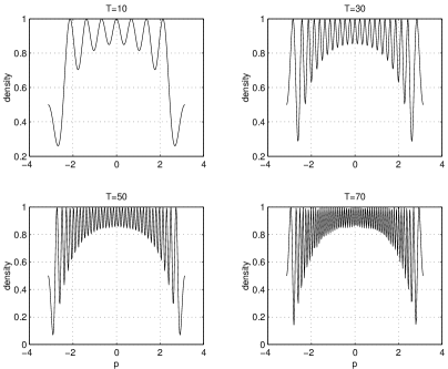
Figure 1: Momentum Space Density functions for $\beta=\frac{\pi}{8}$

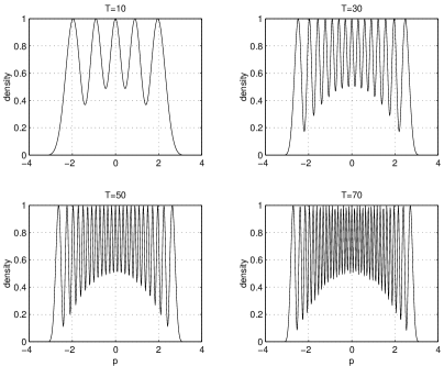
Figure 2: Momentum Space Density functions for $\beta=\frac{\pi}{4}$

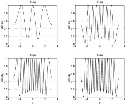
Figure 3: Momentum Space Density functions for $\beta=\frac{3\pi}{8}$

The sequences shows that the densities converge to a limit as time increases. They also illustrate the fact that the momentum space is an attractive representation in which to derive this limit because the domain of the wave functions is constant, $p\in[-\pi,\pi].$ This is in contrast to the real space where the domain expands with time.

VI Conclusions

It has been shown that the momentum space dynamic equations for a quantum walk can be derived using a z transform of the position space equations for the dynamic walk. An exponential representation of the momentum space time evolution operator was derived by using Lie group theory. This enabled the calculation of general momentum space wave functions in terms of Chebyshev polynomials. Some simple calculations of the momentum space probability densities illustrate the convergence of the momentum wave functions to a limit as time increases.

References

- (1) D. Aharanov, A. Ambainis, J. Kempe, U. Vazirani. Quantum walks on graphs. arXiv:quant-ph/0012090, 2000.
- (2) J. Kempe. Quantum walks - an introductory overview. Contemporary Physics and arXiv:quant-ph/0303081v1, 44:307–327, 2003.
- (3) E. Merzbacher. Quantum Mechanics. Wiley, 1998.
- (4) G. Arfken, H. Weber. Mathematical Methods for Physicists. Elsevier, 2005.