Semiclassical approach to Bose-Einstein condensates in a triple well potential

Abstract

We present a new approach for the analysis of Bose-Einstein condensates in a few mode approximation. This method has already been used to successfully analyze the vibrational modes in various molecular systems and offers a new perspective on the dynamics in many particle bosonic systems. We discuss a system consisting of a Bose-Einstein condensate in a triple well potential. Such systems correspond to classical Hamiltonian systems with three degrees of freedom. The semiclassical approach allows a simple visualization of the eigenstates of the quantum system referring to the underlying classical dynamics. From this classification we can read off the dynamical properties of the eigenstates such as particle exchange between the wells and entanglement without further calculations. In addition, this approach offers new insights into the validity of the mean-field description of the many particle system by the Gross-Pitaevskii equation, since we make use of exactly this correspondence in our semiclassical analysis. We choose a three mode system in order to visualize it easily and, moreover, to have a sufficiently interesting structure, although the method can also be extended to higher dimensional systems.

I Introduction

Bose-Einstein condensates form one of the main topics of research at the moment. One reason for this enormous interest is the fact that they combine concepts and techniques from different areas of physics, such as quantum optics, condensed matter physics, molecular physics and quantum chaos. On the experimental side, there has been a remarkable progress in confining and manipulating Bose-Einstein condensates Albi05 ; Schu05a , which has stimulated the theoretical research in the area.

There has been a large number of previous studies analyzing the dynamics of Bose-Einstein condensates in a double well potential using a mean-field approach, the Gross-Pitaevskii equation. In Smer97 Smerzi et al. discussed the occurrence of macroscopic self-trapping within one well. The behavior of the system during an adiabatic change of parameters was studied in 06zener_bec ; Liu03 ; Wu03 and generalizations of the linear two level crossing scenarios and the Landau-Zener formula were analyzed. Another line of investigation considers the mesoscopic regime in which the quantum and the classical, i.e. mean-field descriptions overlap and therefore semiclassical techniques can be used to study the system Milb97 ; Smer00 ; Angl01a ; Angl01b ; Thom03 ; Mahm05 .

In this paper we present a semiclassical technique to analyze the spectral properties of a Bose-Einstein condensate. This method has already been used to describe the vibrational spectra of molecules Sibe96 ; Jaco99 ; Jung02 ; Jung04 and provides an intuitive picture for the at first sight uninterpretable spectra. In this sense, the dynamics of a Bose-Einstein condensate in a triple well potential is analogous to the vibrations of a tri-atomic molecule. Using the geometrical language of classical mechanics to describe the quantum system, we introduce a simple semiclassical method of visualization and classification of the quantum eigenstates which allows a characterization of the dynamics of the system. Furthermore, we investigate how far the correspondence between the mean-field system and the quantum many body system can be extended when the number of particles decreases.

For our studies we consider a Bose-Einstein condensate in a triple well potential, since the technique easily allows us to go beyond the standard double well potential analysis. A triple well potential has a much richer structure 05level3 ; Nemo00 ; Thom03 ; Buon03 ; Fran03 ; Buon04 and the power of the method can be shown without loss of clarity, still allowing a direct visualization of all relevant structures.

II The model

In the following analysis we consider a system consisting of bosonic particles in an external periodic potential $V(\vec{r})=V(\vec{r}+\vec{r}_{\vec{l}})$ with $\vec{r}_{\vec{l}}=l_{1}d_{1}\vec{e}_{1}+l_{2}d_{2}\vec{e}_{2}+l_{3}d_{3}\vec{e}_{3}$, $l_{k}\in\mbox{$\mbox{I}\mbox{N}$}$ and $d_{k}\in{\mathbf{R}}$. If a weak two-particle point-like interaction is assumed, then the Hamiltonian in second quantization can be written as

$${\hat{H}}= \int d^{3}r\;{\hat{{\Phi}}}^{\dagger}(\vec{r})\Bigl{[}-\frac{\hbar^{2}}{2m}\Delta+V(\vec{r})\Bigr{]}{\hat{{\Phi}}}(\vec{r})$$

$$+\frac{g}{2}\int d^{3}r\;{\hat{{\Phi}}}^{\dagger}(\vec{r})\,{\hat{{\Phi}}}^{\dagger}(\vec{r})\,{\hat{{\Phi}}}(\vec{r})\,{\hat{{\Phi}}}(\vec{r})\,.$$ (1)

Here, $m$ is the particle mass, $g=4\pi a_{s}\hbar^{2}/m$ is the coupling constant describing two-body interactions and $a_{s}$ is the s-wave scattering length. For a repulsive interaction, $g$ is positive while for an attractive interaction $g$ takes a negative value. For the rest of the paper we choose scaled units with $\hbar=m=1$. The field operator ${\hat{{\Phi}}}(\vec{r})$ can be expanded in terms of bosonic annihilation operators,

$${\hat{{\Phi}}}(\vec{r})=\sum_{n,m}{\phi_{n,m}}(\vec{r})\,{\hat{a}}_{n,m}\,,$$ (2)

where we assume that the basis functions $\{\phi_{n,m}\}$ of the one-particle Hilbert space are exponentially localized in space and real, as is the case for the Wannier functions Kohn59 . The index $n$ describes basis functions in different wells and we will take into account only three different wells in order to model the three well potential. The second index $m$ labels the excited states within a single well. Assuming Bose-Einstein condensates, we can restrict ourselves to the lowest energy state $m=1$ and neglect higher excited states (see also Milb97 for a careful discussion of this topic for a two well potential). Experimentally such a system was realized in Albi05 for a two well potential but the technique can in principle also be extended to three wells.

Expanding the Hamiltonian in this basis and neglecting fourth order terms in the creation and annihilation operators from different basis functions (modes) yields the well-known Bose-Hubbard Hamiltonian Fish89b restricted to three wells. So, the Hamiltonian can be written in a symmetrized form as

$${\hat{H}}={\hat{H}}_{0}+{\hat{W}}$$ (3)

with

$${\hat{H}}_{0}= \;\omega_{1}\,\frac{{\hat{a}^{\dagger}}_{1}{\hat{a}}_{1}+{\hat{a}}_{1}{\hat{a}^{\dagger}}_{1}}{2}+\omega_{2}\,\frac{{\hat{a}^{\dagger}}_{2}{\hat{a}}_{2}+{\hat{a}}_{2}{\hat{a}^{\dagger}}_{2}}{2}$$

$$+\omega_{3}\,\frac{{\hat{a}^{\dagger}}_{3}{\hat{a}}_{3}+{\hat{a}}_{3}{\hat{a}^{\dagger}}_{3}}{2}+x_{1}\,\biggl{(}\frac{{\hat{a}^{\dagger}}_{1}{\hat{a}}_{1}+{\hat{a}}_{1}{\hat{a}^{\dagger}}_{1}}{2}\biggl{)}^{2}$$

$$+x_{2}\,\biggl{(}\frac{{\hat{a}^{\dagger}}_{2}{\hat{a}}_{2}+{\hat{a}}_{2}{\hat{a}^{\dagger}}_{2}}{2}\biggl{)}^{2}+x_{3}\,\biggl{(}\frac{{\hat{a}^{\dagger}}_{3}{\hat{a}}_{3}+{\hat{a}}_{3}{\hat{a}^{\dagger}}_{3}}{2}\biggl{)}^{2}\,,$$ (4)

$${\hat{W}}= \;-\frac{k_{12}}{2}\,({\hat{a}^{\dagger}}_{1}{\hat{a}}_{2}+{\hat{a}^{\dagger}}_{2}{\hat{a}}_{1})-\frac{k_{23}}{2}\,({\hat{a}^{\dagger}}_{2}{\hat{a}}_{3}+{\hat{a}^{\dagger}}_{3}{\hat{a}}_{2})\,.$$ (5)

Here we neglect a constant energy shift. For convenience, we will choose the nonlinear interaction strengths $x_{j}$ equal for each well in the following sections which is also in accordance with experimental realizations. Such Hamiltonians have already been studied in great detail for the more restrictive two mode model (e.g. in Spek99 ; Angl01b ; Mahm05 ).

The Hamiltonian commutes with the particle number operator ${\hat{N}}={\hat{n}}_{1}+{\hat{n}}_{2}+{\hat{n}}_{3}$ which expresses the conservation of the total number of particles. The symmetrized form is more convenient when considering the semiclassical limit, as will become clear in the next paragraph. Hamiltonians of this kind have been used in molecular physics in order to describe and assign vibrational spectra Jung04 ; Sibe96 . In the molecular case they describe all kinds of vibrational degrees of freedom like stretches, bends, torsions etc. and include various resonant interactions corresponding to different simple rational ratios between the frequencies. The conserved particle number in our case of Eq. (3) corresponds to the polyad-type conserved quantities in the molecular systems.

For the case of 30 particles considered in the following, it is an easy numerical task to diagonalize the Hamiltonian matrix and thus solve the problem. However, one cannot understand the underlying structure of this system from numerical values alone. The aim of this paper is to present a method which allows an easy visual characterization of the eigenvectors of the Hamiltonian, using the close correspondence with the classical system.

II.1 The classical system

Essential for our semiclassical classification and assignment of quantum states is a comparison between the quantum states and the corresponding classical dynamics. To this end, the first step is the construction of the classical Hamiltonian function, which corresponds to the quantum Hamiltonian given in Eqs. (3)–(5). This is done by Heisenberg’s substitution rules Heis25

$${\hat{a}}_{k}\rightarrow\sqrt{I_{k}}e^{i\varphi},\quad{\hat{a}^{\dagger}}_{k}\rightarrow\sqrt{I_{k}}e^{-i\varphi}\,.$$ (6)

There are two different lines of argumentation for this substitution. First, it is exact for the harmonic oscillator where the well known classical Hamiltonian $\omega I$ is obtained by the replacement of the symmetrized product of an annihilation and a creation operator by the classical action. This implies the correspondence

$$I\longleftrightarrow n+\frac{1}{2}$$ (7)

between the classical action $I$ and the quantum number $n$ of the oscillator ($I$ is here measured in units of $\hbar$). This correspondence of Eq. (7) is also a result of the application of the semiclassical Bohr-Sommerfeld quantization rules to the harmonic oscillator. In more general cases we have to generalize the Bohr-Sommerfeld method to the EBK quantization. Then the argument holds for any bound system of any number of degrees of freedom as long as the system is close to integrable (for general background information on semiclassics see Brac97 ). In general, the semiclassical methods give results correct in the lowest two orders in $\hbar$ (orders 0 and 1) and cause errors of order $\hbar^{2}$. The application of the substitution rules of Eq. (6) to the quantum Hamiltonian of Eqs. (3)–(5) gives

$$H(\varphi_{1},\varphi_{2},\varphi_{3},I_{1},I_{2},I_{3})$$

$$=H_{0}(I_{1},I_{2},I_{3})+W(\varphi_{1},\varphi_{2},\varphi_{3},I_{1},I_{2},I_{3})$$

$$=\omega_{1}\,I_{1}+\omega_{2}\,I_{2}+\omega_{3}\,I_{3}+x_{1}\,I_{1}^{2}+x_{2}\,I_{2}^{2}+x_{3}\,I_{3}^{2}$$ (8)

$$\quad-k_{12}\sqrt{I_{1}I_{2}}\,\cos(\varphi_{1}-\varphi_{2})-k_{23}\sqrt{I_{2}I_{3}}\,\cos(\varphi_{2}-\varphi_{3})\,.$$

A Hamiltonian for the same system but expanded in another basis was analyzed in Thom03 . This function can be interpreted as the Hamiltonian of a classical system of three coupled anharmonic oscillators described in action-angle variables $\varphi_{k}\in[0,2\pi)$ and $I_{k}>0$, where $k=1,2,3$. As a method to construct the corresponding classical Hamiltonian, the substitution rules of Eq. (6) always give the correct result since in this direction (quantum $\rightarrow$ classical) the correspondence is unique whenever it exist at all, in contrast to the other direction (classical $\rightarrow$ quantum) with its notorious $\hbar^{2}$ problems. At high excitation (large quantum numbers) there is a second argument for the semiclassical correspondence. The application of a creation or annihilation operator to a number state $|n\rangle$ has the effect

$${\hat{a}}\,|n\rangle=\sqrt{n}\,|n-1\rangle,\quad{\hat{a}^{\dagger}}\,|n\rangle=\sqrt{n+1}\,|n+1\rangle\,.$$ (9)

In the limit of a large quantum number $n$, the difference between $n$ and $n+1$ or $n-1$ is irrelevant in the square roots as well as in the states and the operators can simply be replaced by multiplication with the number $\sqrt{n}$. This argument holds for condensates where a large number of particles goes into a superfluid state which is well described by a mean-field limit. This is in line with the standard argument of semiclassical behavior in the limit of large quantum numbers. Interestingly, for systems of coupled anharmonic oscillators the semiclassical treatment is very good also for low excitation numbers. In this limit, we approach the integrable harmonic limit where the Bohr-Sommerfeld treatment gives the correct result. The experience with molecular systems of the structure of Eqs. (3)–(5) shows that a semiclassical treatment of such systems is globally quite good in most cases.

Accordingly, we base our method of semiclassical assignment on this argument. Semiclassical arguments will be used later first to convert the eigenstates of the many-body Hamiltonian (3) into wave functions on the toroidal configuration space and second to compare these functions with important structures seen in the classical dynamics.

The integrable part $H_{0}$ of the Hamiltonian, which does not contain interactions between the three oscillators, leaves all actions unchanged. In contrast, $W$ changes the values of the actions (particles in the wells) because of its dependence on angles and introduces interactions between the three oscillators. In this sense we call in the following $W$ the interaction part of the Hamiltonian. In the picture of particles in the triple well, $W$ describes tunneling terms between the various wells.

The Poisson bracket between $H$ and the observable

$$K=I_{1}+I_{2}+I_{3}\,,$$ (10)

the total action, is equal to zero, which corresponds to the quantum mechanically conserved number of particles. Note that the numerical value of $K$ differs by $3\cdot 1/2$ from the value of $N$ because of the zero point actions. The symmetry $\{H,K\}=0$ can be used to reduce the number of degrees of freedom from three to two by a canonical transformation. Using the generating function

$$G(\varphi_{1},\varphi_{2},\varphi_{3},J_{1},J_{2},K)\\ =J_{1}(\varphi_{1}-\varphi_{2})+J_{2}(\varphi_{3}-\varphi_{2})+K\varphi_{2}$$ (11)

of the old angles $(\varphi_{1},\varphi_{2},\varphi_{3})$ and the new actions $(J_{1},J_{2},K)$ results in the transformations (together with Eq. (10))

$$\psi_{1}=\varphi_{1}-\varphi_{2}\,,\quad\psi_{2}=\varphi_{3}-\varphi_{2}\,,\quad\vartheta=\varphi_{2}\,,$$

$$I_{1}=J_{1}\,,\quad I_{3}=J_{2}\,,$$ (12)

where $(\psi_{1},\psi_{2},\theta)$ are the new angles conjugate to $(J_{1},J_{2},K)$.

The Hamiltonian in the new coordinates is given by

$$H= \;\omega_{1}\,J_{1}+\omega_{2}\,(K-J_{1}-J_{2})+\omega_{3}\,J_{2}$$

$$+x_{1}\,J_{1}^{2}+x_{2}\,(K-J_{1}-J_{2})^{2}+x_{3}\,J_{2}^{2}$$

$$-k_{12}\sqrt{J_{1}(K-J_{1}-J_{2})}\,\cos\psi_{1}$$

$$-k_{23}\sqrt{J_{2}(K-J_{1}-J_{2})}\,\cos\psi_{2}\,,$$ (13)

with corresponding equations of motions

$$\dot{\psi}_{1} =(\omega_{1}+2x_{1}J_{1})-(\omega_{2}+2x_{2}(K-J_{1}-J_{2}))$$

$$\quad-\frac{k_{12}}{2}\Biggl{[}\,\sqrt{\frac{K-J_{1}-J_{2}}{J_{1}}}-\sqrt{\frac{J_{1}}{K-J_{1}-J_{2}}}\;\Biggr{]}\cos\psi_{1}$$

$$\quad+\frac{k_{23}}{2}\sqrt{\frac{J_{2}}{K-J_{1}-J_{2}}}\cos\psi_{2}\,,$$ (14)

$$\dot{\psi}_{2} =(\omega_{3}+2x_{3}J_{2})-(\omega_{2}+2x_{2}(K-J_{1}-J_{2}))$$

$$\quad-\frac{k_{23}}{2}\Biggl{[}\,\sqrt{\frac{K-J_{1}-J_{2}}{J_{2}}}-\sqrt{\frac{J_{2}}{K-J_{1}-J_{2}}}\;\Biggr{]}\cos\psi_{2}$$

$$\quad+\frac{k_{12}}{2}\sqrt{\frac{J_{1}}{K-J_{1}-J_{2}}}\cos\psi_{1}\,,$$ (15)

$$\dot{J}_{1} =-k_{12}\,\sqrt{J_{1}(K-J_{1}-J_{2})}\,\sin\psi_{1}\,,$$ (16)

$$\dot{J}_{2} =-k_{23}\,\sqrt{J_{2}(K-J_{1}-J_{2})}\,\sin\psi_{2}\,.$$ (17)

The classical configuration space is a two dimensional torus spanned by the two angles $\psi_{1}$ and $\psi_{2}$. In order to compare the classical and the quantum system we have to represent the states as wave functions on the classical configuration space. The way to do this will be described in the following section.

II.2 The quantum mechanical configuration space

The angle variables can be introduced in the quantum system by using the set of functions

$$|\varphi_{1},\varphi_{2},\varphi_{3}\rangle=\!\!\!\!\!\!\!\sum_{n_{1},n_{2},n_{3}\geq 0}\!\!\!\!\!\!\!e^{i(n_{1}\varphi_{1}+n_{2}\varphi_{2}+n_{3}\varphi_{3})}\,|n_{1},n_{2},n_{3}\rangle\,,$$ (18)

first introduced in molecular spectroscopy by Sibert and McCoy Sibe96 . These functions are similar to the Bargmann states studied in Angl01b in the context of a Bose-Einstein condensate. This relation is well-known from the context of infinite lattices. There, the sum is taken from $-\infty$ to $\infty$ and corresponds to the representation of Bloch functions in terms of Wannier functions. The angle variables $\varphi_{1}$, $\varphi_{2}$ and $\varphi_{3}$ span the Brillouin zone. However, in this example these functions are not orthogonal due to the fact that for fixed $N$ the sum is finite,

$$\langle\varphi^{\prime}_{1},\varphi^{\prime}_{2},\varphi^{\prime}_{3}|\varphi_{1},\varphi_{2},\varphi_{3}\rangle\\[5.69054pt] =\!\!\!\!\!\!\!\sum_{n_{1}+n_{2}+n_{3}=N}\!\!\!\!\!\!\!e^{-i(n_{1}(\varphi_{1}-\varphi^{\prime}_{1})+n_{2}(\varphi_{2}-\varphi^{\prime}_{2})+n_{3}(\varphi_{3}-\varphi^{\prime}_{3}))}\,.$$ (19)

For a large particle number $N$ the scalar product converges to a delta-comb. There is a considerable deviation for the value of $N=30$, which can play an important role when matrix elements are calculated. But here we use these functions only for visualization and not for further algebraic manipulations. The eigenfunctions of (3) have the form

$$|{\Phi}\rangle=\!\!\!\!\!\!\!\sum_{n_{1}+n_{2}+n_{3}=N}\!\!\!\!\!\!\!c_{n_{1},n_{2},n_{3}}\,|n_{1},n_{2},n_{3}\rangle\,.$$ (20)

The coefficients $c_{n_{1},n_{2},n_{3}}$ can be obtained by a numerical diagonalization in the number basis $|n_{1},n_{2},n_{3}\rangle$. The eigenstates in the angle representation (18), i.e. the wave functions, are given by a Fourier series:

$$\langle\varphi_{1},\varphi_{2},\varphi_{3}|{\Phi}\rangle=\!\!\!\!\!\!\!\sum_{n_{1}+n_{2}+n_{3}=N}\!\!\!\!\!\!\!c_{n_{1},n_{2},n_{3}}\,e^{i(n_{1}\varphi_{1}+n_{2}\varphi_{2}+n_{3}\varphi_{3})}\,.$$ (21)

Finally, we can reduce the number of degrees of freedom in this representation by using the same coordinate transformation as in the classical case of Eq. (12). This leads to the expression

$${\Phi}(\psi_{1},\psi_{2})=\langle\psi_{1},\psi_{2}|{\Phi}\rangle\\ =e^{iN\vartheta}\sum_{n_{1}+n_{3}\leq N}c_{n_{1},N-n_{1}-n_{3},n_{3}}\,e^{i(n_{1}\psi_{1}+n_{3}\psi_{2})}\,.$$ (22)

The global phase factor $e^{iN\vartheta}$ can be ignored in the following considerations. It must be emphasized that the sum includes only a finite number of terms due to the finite number of combinations of numbers $n_{1}$, $n_{2}$ and $n_{3}$ which sum to $N$. Therefore the Fourier expansion in Eq. (22) has only a finite resolution. For a very small value of $N$, this sum has just a few terms, so that only the coarse grain structure can be explored; accordingly, the eigenfunctions ${\Phi}(\psi_{1},\psi_{2})$ show only diffuse structures. In our example, the configuration space of the reduced system is the two dimensional torus $T^{2}$ with total volume $4\pi^{2}$. The total number of basis states for a given number of particles $N$ is $L=(N+1)(N+2)/2$. Accordingly, the eigenfunctions which are linear combinations of the $L$ basis functions can only show patterns with a resolution of the order $4\pi^{2}/L$ in the area or a resolution of the order $2\pi/N$ in each direction. With $N=30$ we have $L=496$ eigenstates, giving a resolution of approximately $0.07\pi$ in each direction.

The reinterpretation of the expansion of an eigenstate into number states as a Fourier series on the toroidal configuration space has the following semiclassical interpretation, where we write for the moment $\hbar$ explicitly into the equations: If one naively quantizes the classical canonical variables $(\varphi_{k},I_{k})$ using the Schrödinger quantization $[\hat{\varphi}_{k},\hat{I}_{l}]=i\hbar\delta_{kl}$, which imposes $\hat{I}_{k}=(i\hbar)^{-1}\partial/(\partial\varphi_{k})$, then functions $f(\varphi_{1},\varphi_{2},\varphi_{3})$ can be interpreted as wave functions in coordinate space. Of course, the Schrödinger quantization is correct only in Cartesian coordinates and it does not commute with canonical transformations, in general yielding errors of the order of $\hbar^{2}$. Therefore the results have to be interpreted semiclassically. Note that due to our symmetric introduction of the quantum-classical correspondence in Eq. (7), the errors to first order in $\hbar$ cancel identically. Because of these considerations we call the wave function from Eq. (22) the semiclassical wave function.

In many semiclassical investigations, Husimi functions are used to relate quantum wave functions of eigenstates to structures in the classical phase space. This is the appropriate and natural procedure if the usual position and momentum coordinates are used. It is less clear and in addition not necessary in our case where the whole dynamics is treated in action-angle variables. Let us explain this point in some detail: The description of the system by a Hamiltonian of the functional structure of Eqs. (3)–(5) in the quantum case or Eq. (II.1) in the classical case only makes sense for bound systems, it is not appropriate to describe scattering systems. Therefore we restrict the following discussion to bound states only. For any bound eigenstate in the standard position space, there must be the same amount of wave running in one direction and in the opposite direction, otherwise it would not be a bound stationary state. Accordingly, the wave function can be chosen real. The phases of the wave function do not play any important role and do not help for the classification of the states. The canonically conjugate momenta have continuous values and Wigner or Husimi functions are defined without any problem on the classical phase space and indicate in many cases to which structure in the classical phase space some particular quantum state belongs.

The situation is very different in action angle variables. Here the configuration space is a torus with its very different global topology. This causes great difficulties to define the usual Wigner or Husimi functions. Because of the periodicity of the configuration coordinates, the corresponding canonically conjugate variables (here the actions) only have discrete values in the quantum dynamics. This makes it very tricky to convert the wave function into something defined on the continuous classical phase space. On the other hand, we do not really need to do this, since we have the following simpler method to squeeze out of the wave functions information on the classical actions. Waves propagating in one direction on a torus always return to the starting point. Accordingly, wave functions for a bound state can have – and in fact in most cases do have – strong running wave contributions and the phase of the function is essential and will be analyzed to help in the classification of the state. In a semiclassical spirit the phase of a wave function can be interpreted as a classical action integral and accordingly the gradient of the phase function gives the value of the canonically conjugate momentum which in this case is the action. If there is a sufficiently large patch of configuration space where the phase function comes close to a plane wave, then its gradient indicates the value of the actions which is represented by this part of the wave function. This provides a kind of lift of the wave function from configuration space into phase space. If there are closed loops on the torus along which the phase function is very regular (and this usually happens along density crests which run along the classical organizing center as will be explained in detail in section IV) then we interpret this as representing a motion of almost constant action along this loop. This idea is used to get longitudinal quantum numbers introduced in section IV.

III Classical dynamics and coupling schemes

Before we relate individual quantum states to guiding centers of the classical dynamics, we must get an overview of the classical dynamics and its skeleton. As an example, we discuss the classical dynamics for $N=30$, i.e. for the value $31.5$ of the classically conserved total action $K$. In the following, we choose parameter values $\omega_{1}=-\omega_{3}=0.1$, $\omega_{2}=0$, $x_{1}=x_{2}=x_{3}=0.1$ and $k_{1,2}=k_{2,3}=0.5$, which lead to a quantum mechanical energy interval of $[23.907,96.393]$. The classical reduced system exists in the energy interval $[22.476,99.1]$. Furthermore, we measure all energies with respect to the quantum mechanical ground state of $H$ in Eq. (3), i.e. we subtract the quantum mechanical zero point $H_{0}(1/2,1/2,1/2)=0.075$ from the classical energies in order to facilitate the comparison between classical and quantum dynamics. To represent the classical dynamics graphically, we show Poincaré sections in planes $\psi_{1}=0$ with positive orientation $\dot{\psi}_{1}>0$. If an initial condition $(\psi_{2},J_{2})$ is chosen in the Poincaré section, then we first have to reconstruct the four corresponding coordinates in the phase space in order to start a trajectory of the flow through this point. The two coordinates $\psi_{2}$ and $J_{2}$ coincide with the given coordinates in the domain of the Poincaré map. The coordinate $\psi_{1}$ is obtained by the intersection condition and the remaining coordinate $J_{1}$ is calculated by an inversion of the Hamiltonian function (II.1) with respect to the coordinate $J_{1}$ for a fixed value of the energy and for the known values of the other three coordinates. Here some care is necessary since this inverse function is multivalued. First we fix one orientation of the domain, i.e. we always search for solutions with $d\psi_{1}/dt>0$. In principle there can be several solutions with the same orientation and then it is necessary to ensure that all initial points used belong to the same branch. Poincaré sections in planes $\psi_{2}=\text{constant}$ look very similar to the ones in planes $\psi_{1}=\text{constant}$. Therefore it is sufficient to restrict ourselves to sections in $\psi_{1}=0$ only.

If the whole dynamics were governed by $H_{0}$, then all actions would be constants of motion and all Poincaré sections would be foliated by invariant lines $J_{2}=\text{constant}$. Including the interaction $W$ between the wells (modes) into the dynamics has the following effects. In regions of the phase space, where none of the resonances contained in $W$ has an important effect, the dynamics is in the KAM regime (see the extensive discussion of soft chaos in chapter 9 of Gutz90 ) and a large fraction of the phase space volume is still filled by invariant lines, which are continuous deformations of the invariant surfaces $\vec{J}=\text{constant}$ of the unperturbed $H_{0}$ dynamics. We call such invariant surfaces primary tori. This happens mainly in regions of phase space where the effective frequencies

$$\omega^{\text{eff}}_{j}=\frac{\partial H_{0}}{\partial I_{j}}$$ (23)

are far from simple rational ratios, for which there is a corresponding resonance coupling in $W$, as explained in the next paragraph. For our particular choice of coupling terms in $W$, only 1:1 resonances are relevant.

The effect of the coupling terms between the different modes can be described in the following way. Each term contains a cosine function whose argument is a difference between angles of the original degrees of freedom or one angle of the reduced system, see Eqs. (II.1) and (II.1). Because in our special case the arguments are differences of two angles with the same weight, we say that these terms describe 1:1 resonant interactions between the two degrees of freedom. The right hand sides of the Hamiltonian equations of motion (14) and (15) for the angles $\psi_{k}$ ($k=1,2$) of the reduced system,

$$\frac{{\rm d}\psi_{k}}{{\rm d}t}=\frac{\partial H_{0}}{\partial J_{k}}+\frac{\partial W}{\partial J_{k}}\,,$$ (24)

contain two contributions. The first consists of the difference of two effective frequencies from Eq. (23), and the second is the derivative of the coupling terms with respect to the action, which contains cosine functions. First, let us assume that we change some parameter, e.g. $k_{1,2}$, to see how coupling sets in. Further we assume that the difference between the effective frequencies, i.e. the angle independent term on the right hand side, is different from zero. Let us say it has the value $\nu\neq 0$. For a small value of $k_{1,2}$ the angle dependent terms are not able to cancel $\nu$ regardless of the value of the angles. The angle dependent terms have the maximal absolute value for angle values $0$ and $\pi$ because of the dependence on cosine functions. When $k_{1,2}$ increases, then at one point it reaches a value, where the angle dependent terms are just able to cancel $\nu$. Then the angle $\psi_{k}$ of the reduced system stops, $\psi_{k}(t)=\text{constant}$, and we call this frequency locking. This necessarily happens for angle values where the cosine functions have maximal absolute value, i.e. where the angles are 0 or $\pi$. Whether the appropriate angle values are 0 or $\pi$ depends on the signs of $\nu$ and of the terms in front of the cosine functions. When the value of $k_{1,2}$ is further increased, then there is a whole interval of angle values where locking is possible. The actual dynamics of the locked motion then performs small oscillations around the angle values 0 or $\pi$. This will be seen in the numerical results of the classical dynamics. In the quantum dynamics the fluctuations around the coupling point of the angles are quantized and give rise to a discrete set of transversal quantum numbers, see section IV.

If only one of these resonant couplings is strong, then the dynamics is still close to integrable, and a large part of the phase space volume is filled by invariant tori, which show up as invariant lines in the Poincaré sections. However, due to the rearrangement of phase space structures by the resonant coupling, the invariant surfaces in phase space are no longer primary tori, i.e. are no longer continuous deformations of invariant surfaces of the $H_{0}$ dynamics. Large bundles of secondary tori appear which are organized around periodic orbits (in this case stable, elliptic) representing the guiding centers for the new nonlinear modes. There are also corresponding unstable periodic orbits, which in the integrable case are represented by separatrix crossings in Poincaré sections. In the nonintegrable cases, the separatrices break and turn into homoclinic tangles, which become the central structures of chaotic strips. However, if only one resonant coupling has a strong effect and the others are not important, then the chaos strips are very thin and they still appear almost like separatrices.

If two or more linearly independent resonant couplings are strong, then chaos on large scales can appear. These regions in phase space are resonance overlap zones Chir79 . However, also in strongly chaotic regions of phase space there are still simple short periodic orbits (in this case unstable, normal hyperbolic or inverse hyperbolic) which act as guiding centers of the flow. Then the dynamics is chaotic but nevertheless the flow follows some guiding center on the average. This average flow is relevant for the comparison with quantum dynamics. Thus, also in the classically chaotic case we may find surprisingly simple and clean structures in a large part of the quantum wave functions. In such cases it can be appropriate to imagine simple idealized classical guiding centers and interpret the quantum states as quantum excitations of these idealized structures.

Let us give a short estimate of the size of structures which are relevant for our semiclassical considerations. The range of action values is limited between 0 and $K$ due to Eq. (10), the angle can vary over an interval of length $2\pi$. For each particular plot only a part of this range is energetically accessible in reality. Accordingly the size of the Poincaré section is limited by $2\pi K$. For semiclassical investigations structures of a size of $\hbar$ or larger are relevant. We always use units in which $\hbar$ has the numerical value 1 and also the values of all actions should be interpreted as being given in units of $\hbar$. Therefore structures in our Poincare plots are of interest in the following, if their size is at least in the order of one unit of action or has a relative size of $1/K$ compared to the size of the maximally possible domain of the map.

We perform almost all our calculations for the reduced system. On the other hand, the real object of interest is the original system of particles in three wells. Therefore we need a fast and easy method to transfer statements about the reduced system into the corresponding statements about the original system. We have called this procedure the lift in the previous work on molecular systems Jung04 ; Jaco99 ; Jung02 . Let us assume a trajectory of the reduced system is given and we want to reconstruct the corresponding trajectory of the original system. The first step of the procedure is the reconstruction of the cyclic angle. It is done rigorously by using the Hamiltonian equation of motion

$$\frac{{\rm d}\vartheta}{{\rm d}t}=\frac{\partial H}{\partial K}\,.$$ (25)

The right hand side of this equation does not depend on $\vartheta$ but only on the known values of the other coordinates as function of time. Accordingly we get $\vartheta(t)$ by a simple integration with respect to time. The experience with the molecular systems has shown that normally it is sufficient to approximate $\vartheta(t)$ by $t$ times a constant effective frequency. In our case $\vartheta$ is the only fast variable of the whole system and describes a fast oscillation superimposed on the motion of the whole system. The initial value $\vartheta(0)$ is rather irrelevant. In contrast, the variables of the reduced system are slow variables describing the relative motion between the various degrees of freedom of the original system. The next step of the lift procedure is to undo the canonical transformation and to go back to the coordinates of the original system. In this second step the advantage of choosing the new actions equal to some of the old actions becomes evident. The knowledge of the actions in the reduced system and of the constant value of $K$ gives immediately the values of the old actions, i.e. the values of the particle numbers in the three wells. Because of this simple connection between the actions of the reduced system and the actions of the original system we will switch very freely between the reduced and the original system in the following considerations.

In our case we have in the interaction part $W$ of the Hamiltonian 1:1 couplings between the degrees of freedom 1 and 2 and between 2 and 3 respectively. Indirectly this also implies a 1:1 coupling between the degrees of freedom 1 and 3. Accordingly, we have the following coupling schemes:

Figure 1: The classical reduced system for energy $E=55$. (a) Poincaré plot in the plane $\psi_{1}=0$ for variables $\psi_{2}$ and $J_{2}$ with $J_{1}$ fixed by energy conservation. (b) Trajectory in a primary torus in the lower region of (a) for initial values $(\psi_{1},\psi_{2},J_{2})=(0,\pi,7.5)$. (c) Trajectory in a primary torus in the upper region of (a) for initial values $(0,0,20.6)$. The points of the trajectories are given in equidistant time intervals $\Delta t=0.01$ in order to indicate the velocity by the distance between neighboring points.

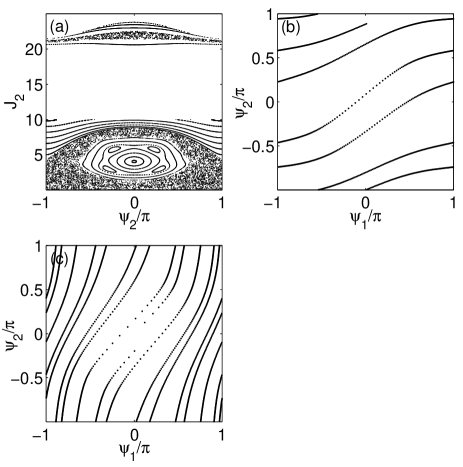
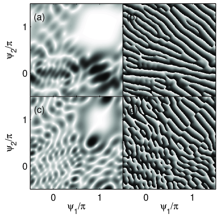
Type (A) : If the effective frequencies are not very close to each other, then no interaction term can cause frequency and phase coupling, and all three modes run independently with their own effective frequency. This is the KAM regime with many primary tori, where the motion is of quasiperiodic type with three independent frequencies. The organization center of the reduced system is the complete configuration space $T^{2}$. In Poincaré plots, we see many invariant lines which are continuous deformations of horizontal lines $J_{2}=\text{constant}$, i.e. of the invariant lines belonging to $H_{0}$. This type of motion appears mainly in the middle of the accessible energy interval for a given particle number. In Fig. 1 we give some numerical results for the energy $E=55$. Part (a) shows the Poincaré section and parts (b) and (c) show two segments of trajectories in the reduced configuration space. The domain of the Poincaré map in (a) consists of two parts. The range of $J_{2}$ values between approximately 10.2 and 20.5 is not accessible at this energy. At values of $J_{2}$ around 9, we see many primary tori. A segment (five revolutions in direction of $\psi_{1}$) of a typical trajectory belonging to one of them is shown in part (b) of the figure. In the long run, the trajectory fills the whole configuration space quasiperiodically. In these primary tori the action $J_{2}$ is smaller than the action $J_{1}$, so that the trajectories move faster in $\psi_{1}$ direction than in $\psi_{2}$ direction. The opposite happens on the primary tori lying around $J_{2}$ values of 21. Here the $J_{2}$ action is largest and therefore the quasiperiodic trajectories run with higher speed in the $\psi_{2}$ direction. (For a numerical example, see a trajectory segment in Fig. 1(c)). The other structures seen in Fig. 1(a) belong to other types of motion, discussed below.

Type (B) : If the effective frequencies of modes 2 and 3 are close but that of the first mode is not close, then we expect that modes 2 and 3 are locked but mode 1 is independent. The motion is then quasiperiodic with two independent frequencies. The organization center in the reduced system is a one dimensional curve with $\psi_{2}=\text{constant}$. In Poincaré plots in the plane $\psi_{1}=0$, we see secondary islands. This motion appears mainly for high energies. Figure 2 gives some numerical results for $E=80$. Part (a) shows a Poincaré section, again in the plane $\psi_{1}=0$, and part (b) shows two periodic orbits in the configuration space. The motion at the upper end of the accessible energy interval is close to integrable. At a very high energy, motion in $\psi_{1}$ direction is preferred, since the linear frequency $\omega_{1}$ of original mode 1 is higher than the frequency $\omega_{3}$ of mode 3. For decreasing energy, the KAM island around the center at $\psi_{2}=0$ increases in size while the one around $\psi_{2}=\pi$ decreases. The central periodic orbit around $\psi_{2}=0$ remains stable for energies down to approximately $E=45$, while the other one soon becomes unstable and its KAM island disappears. In Fig. 1(a) we see clearly the large KAM island belonging to the organization center $\psi_{2}=0$, with center at $J_{2}=4$.

Figure 2: (Color online) The classical reduced system for an energy $E=80$. (a) Poincaré plot as in Fig. 1(a). (b) Periodic orbits crossing the Poincaré section in the centers of the KAM islands (black) for initial values $(\psi_{1},\psi_{2},J_{2})=(0,0,1.3)$ and at the border (green) for initial values $(0,\pi,2.6)$.

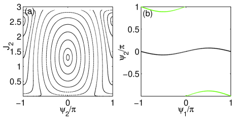
In contrast to the idealized organization center $\psi_{2}=0$, the exact one is a periodic trajectory running in $\psi_{1}$ showing small wiggles in $\psi_{2}$ direction around the average value $\psi_{2}=0$. However for our considerations it is simpler and completely satisfactory to replace this true organization center, the true periodic orbit, by an idealized organization center, for which we just take the straight line $\psi_{2}=0$. The reader might remember the previous discussion of the onset of angle coupling and the values of the angles at which coupling sets in. In the spirit of this previous discussion we define the idealized organization center as the subset of the configuration space defined by the angle restrictions exactly at the onset of the corresponding coupling scheme. Also the idealized semiclassical wave functions are given with respect to the corresponding idealized organization center.

Type (C) : If the effective frequencies of modes 1 and 2 are close, but that of the third mode is not close, then we expect that modes 1 and 2 are locked but mode 3 is independent. Then the motion is again quasiperiodic with two independent frequencies. In the reduced system, the organization center is a one dimensional curve which can be idealized by a line $\psi_{1}=\text{constant}$, where the constant usually is $0$ or $\pi$ according to the discussion in the beginning of this section. The periodic orbit itself running in the $\psi_{2}$ direction is almost impossible to find in Poincaré maps with plane of intersection $\psi_{1}=0$, since it violates the transversality of the map. However, when it is stable, then there is a bundle of invariant tori around it. In Poincaré plots in the planes $\psi_{1}=0$, these invariant tori appear as lines extending over all values of $\psi_{2}$. In Fig. 1(a) they are the lines at the highest values of $J_{2}$. In Fig. 3, we show some numerical results at energy $E=40$. Part (a) shows the Poincaré map and parts (b) and (c) show trajectories in configuration space. In Fig. 3(a) the lines at small values of $J_{2}$ belong to the tori around the organization center $\psi_{1}=0$. Figure 3(b) shows a segment of a typical quasiperiodic orbit on one of these tori. While running monotonously in the negative $\psi_{2}$ direction, it oscillates in $\psi_{1}$ around the value 0.

Figure 3: (Color online) The classical reduced system for an energy $E=40$. (a) Poincaré plot as in Fig. 1(a). (b) Quasiperiodic orbit with initial values $(\psi_{1},\psi_{2},J_{2})=(0,\pi,2)$. (c) Two periodic orbits: one oscillating along the diagonal with starting point $(0,0,14.4)$ (black) and the other rotating around the line $\psi_{1}=\psi_{2}+\pi$ (green) with starting point $(0,\pi,11.5)$.

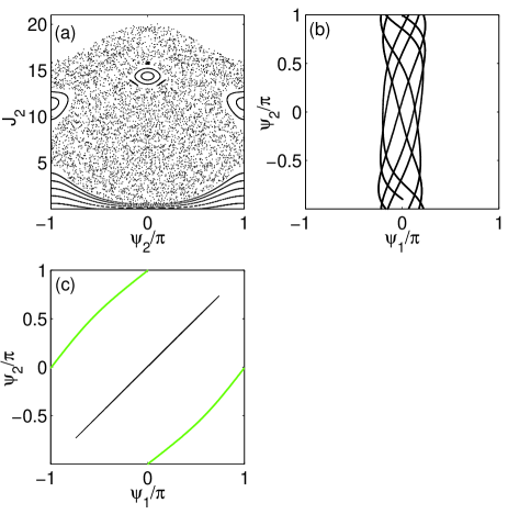
Type (D) : If the effective frequencies of modes 1 and 3 are very close, then also the weak indirect tunneling processes between modes 1 and 3 can cause coupling. If the frequency of mode 2 is far from this common frequency, then mode 2 runs independently. The corresponding organization center in the reduced system is the line $\psi_{1}=\psi_{2}+\text{constant}$, where again this constant is usually 0 or $\pi$. In Poincaré plots in planes $\psi_{1}=0$, we see secondary islands. In Fig. 3(a), the two KAM island of moderate size with centers at $\psi_{2}=0$, $J_{2}=14$ and $\psi_{2}=\pi$ and $J_{2}=11.5$ respectively represent this type of motion. The two periodic orbits belonging to the centers of these two KAM islands are shown in Fig. 3(c). One oscillates along the diagonal and the other rotates around along the line $\psi_{1}=\psi_{2}+\pi$.

Type (E) : If all three effective frequencies are close, then there are two possibilities:

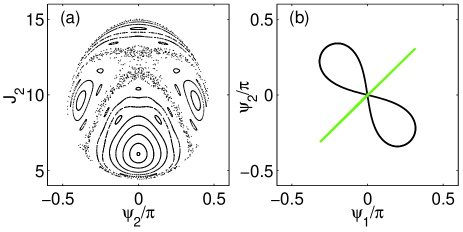
(E1): There is coupling between all three modes and the idealized organization center in the configuration space of the reduced system is a (fixed)point. The actual trajectories oscillate around this coupling point and the relative angles $\psi_{k}$ do not rotate around the whole configuration torus. This behavior, which dominates at very small energy, is shown in Fig. 4 at energy $E=27$. Only a limited range of $\psi_{2}$ values around the point zero is energetically accessible. The same also holds for $\psi_{1}$. Rotations around the configuration torus in either direction or the diagonal become possible only for a higher energy. One of the organizing centers is represented in the Poincaré plot by a stable fixed point which lies at the center of the large KAM island shown in Fig. 4(a), and which is shown in configuration space in Fig. 4(b) as the figure-of-eight orbit mainly oscillating in the antidiagonal direction. The other organizing center is an unstable periodic orbit belonging to the unstable fixed point near $\psi_{2}=0$, $J_{2}=12$ in the Poincaré plot. In the configuration space plot of Fig. 4(b), it is the orbit oscillating in the diagonal direction. At this energy, all trajectories in configuration space oscillate around the point $(0,0)$, which acts as point organizing center. The two periodic orbits of Fig. 4(b) then act as guiding structures for these fluctuations around the organizing center. Topologically speaking, all trajectories are contractible to a point on the configuration torus at very low energy. At the lower end of the accessible energy interval, the dynamics starts as almost integrable and for this case the invariant manifolds of the unstable fixed point mentioned above lie close to a figure-of-eight shape separatrix in the Poincare section. For increasing energy the system moves further away from integrable and the separatrix breaks and turns into a homoclinic tangle which is the central structure of a chaos strip. In Fig. 4(a) for energy $E=27$ this chaotic layer still has moderate size. For higher energy it grows rapidly and turns into the large chaotic sea seen in Fig. 3(a) at energy $E=40$.

Figure 4: (Color online) Classical reduced system for energy $E=27$. (a) Poincaré plot as in Fig. 1(a). (b) Trajectories through the stable fixed point (black, double loop) with initial values $(\psi_{1},\psi_{2},J_{2})=(0,0,6.1)$, and the unstable fixed point (green, along the line $\psi_{1}=\psi_{2}$) with initial values $(0,0,12.1)$.

(E2): The couplings break and reestablish intermittently, and the dynamics shows large-scale chaos. The appearance of chaos in the case of two independent resonant interactions becoming active is a demonstration of Chirikov’s point of view of chaos being caused by resonance overlap Chir79 . In Poincaré plots, we see large-scale chaos and eventually embedded in it remnants of islands and regular structures. The beginning of chaos for small energies can be seen in Fig. 4(a); chaos on a large scale is evident in Figs. 1(a) and 3(a).

IV Classification of semiclassical wave functions

In this section, we show examples of wave functions belonging to the various classes of motion described in the previous section. Our method of classification has been developed in Jung04 ; Jaco99 ; Jung02 ; Sibe96 especially for Hamiltonians given quantum mechanically in raising and lowering operators and classically in action-angle variables. An analysis in a similar spirit of wave functions in the usual position space is rather common in molecular physics, two representative examples are Jost99 ; Azza03 . In contrast to the procedure in action-angle space, the procedure in regular position space can be extended to scattering resonances, see Gome89 .

Our strategy of classification is as follows: First we expand the eigenstates $|{\Phi}\rangle$ in the representation $|\psi_{1},\psi_{2}\rangle$, according to Eq. (22). This representation of the eigenstates in the reduced configuration space is in complete analogy to the classical configuration space spanned by the angle variables $\psi_{1}$ and $\psi_{2}$ and therefore allows a direct comparison between the classical and quantum system. We refer to these eigenfunctions ${\Phi}(\psi_{1},\psi_{2})$ as the semiclassical wave functions in order to indicate this resemblance. We then check whether the density of the semiclassical wave function in the reduced configuration space resembles the structure of one of the organization centers described in the previous section (types (A) – (E2)). I.e. we check, whether the density is distributed over the whole configuration space without clear nodal structures (type (A)), is concentrated along a few lines in the $\psi_{1}$ direction (type (B)), in the $\psi_{2}$ direction (type (C)) or in the diagonal direction (type (D)), is organized around the point center $(0,0)$ (type (E1)) or shows random interferences between the pattern of different organization centers leading to irregular structures (type (E2)).

We call states, for which the density is located in a single crest along the organizing center, a transverse ground state to this organization center. In transversely excited states, the density is concentrated along various copies of the organization center, where these various copies are displaced relatively to each other and the wave function shows nodal structures between them. In addition, we look for the phase advance in directions in or parallel to the organization structure. The phase function must be continuous along curves which do not cross nodal lines. Recall that the phase function can have singularities only in zero points of the density. Accordingly, the curve along a crest of high density must be a curve of continuous phase. Then the phase advance of such a curve must be some integer multiple of $2\pi$, say $\mu_{l}\cdot 2\pi$, and this number $\mu_{l}$ serves as one quantum number of the state. These longitudinal quantum numbers, together with the transverse quantum numbers given by the nodal structures, provide a complete set of quantum numbers characterizing the state relative to its organization center. We expect all states which can be related to an organization center to be close to a product of a plane wave in the longitudinal direction of this organization center and an oscillator function in transverse directions.

In states belonging to classically chaotic motion, we do not see a simple and clear pattern in the density nor in the phase. Accordingly we are not able to give any assignment by quantum numbers to such states.

In the following, the eigenstates ${\Phi}_{k}$, $k=1,\,2,\,\dots 496$ are sorted by increasing energy starting with the label 1 for the eigenstate with lowest energy.

Point organization center (Type (E1))

We start our analysis of the semiclassical wave functions at the lower end of the accessible energy interval. Since the Hamiltonian is dominated by quadratic anharmonicities, the smallest energy is realized by distributing the total excitation of 30 quanta (particles) evenly over the 3 basis modes (potential wells). In the classical picture, this corresponds to the case where all three actions $I_{k}$ are close to each other. Thus the three effective frequencies (23) are very similar and frequency and phase locking is easily established by the resonant coupling terms in the Hamiltonian as explained in the beginning of section III. In the classical configuration space, this mechanism restricts the trajectories to a small region of configuration space (cf. Fig. 4). This behavior is confirmed in the quantum case. Here, the wave functions are organized around a point, as can be seen in Fig. 5, where the ground state and various excited states are plotted. State ${\Phi}_{1}$ is the ground state in this class. In this case the ground state of an organization center coincides with the energetic groundstate ${\Phi}_{1}$ of the whole system, but we will assign also a groundstate for the other types of guiding centers. The state ${\Phi}_{2}$ is the first transversal excitation in the antidiagonal direction, while the state ${\Phi}_{3}$ represents the first transversal excitation in the diagonal direction. The state ${\Phi}_{4}$ represents the second transversal excitation in the antidiagonal direction, and the state ${\Phi}_{5}$ is the combination of one transverse excitation in the diagonal and one in the antidiagonal direction. State ${\Phi}_{9}$ is the fourth excitation in the antidiagonal direction. A point center does not have any longitudinal directions. Accordingly, there are no phase advances in longitudinal directions to be counted for the assignment and any state of this class is characterized by the two transverse excitation numbers $(\mu_{td},\mu_{ta})$, one in the diagonal direction and one in the antidiagonal direction. Thus we show only the density plots without the phases in Fig. 5.

In this scheme, the six states ${\Phi}_{1}$, ${\Phi}_{2}$, ${\Phi}_{3}$, ${\Phi}_{4}$, ${\Phi}_{5}$ and ${\Phi}_{9}$ have quantum numbers $(0,0)$, $(0,1)$, $(1,0)$, $(0,2)$, $(1,1)$ and $(0,4)$, respectively.

Figure 5: Gray scale plot of the squared modulus of the (a) ground state ${\Phi}_{1}(\psi_{1},\psi_{2})$ and the excited states (b) ${\Phi}_{2}$, (c) ${\Phi}_{3}$, (d) ${\Phi}_{4}$, (e) ${\Phi}_{5}$ and (f) ${\Phi}_{9}$. White color corresponds to low density and black to the highest density. The range of the $\psi_{k}$ is $[-\pi/2,3\pi/2]$.

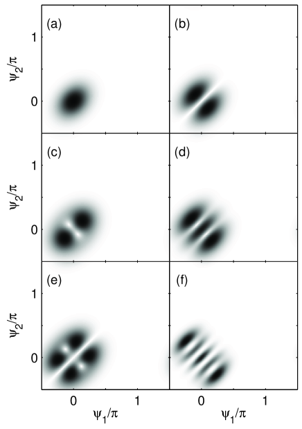
Note that the direction of excitation corresponds to the direction of oscillation of the classical periodic orbits shown in Fig. 4(b). The classical periods of these two orbits are $T_{a}=6.112$ for the antidiagonal one and $T_{d}=3.502$ for the diagonal one. The quantum excitations in the corresponding direction increase the energy of the state by the classical frequency $\omega=2\pi/T$, where $T$ is the period of the orbit taken at an intermediate energy.

The quantum-classical correspondence can be described in the following way: All three original modes are frequency locked and the phases fluctuate around the coupling point. The motion is similar to the one in a two dimensional anharmonic oscillator centered around the point $(0,0)$. This oscillator has its own normal modes and the states presented in Fig. 5 can be interpreted as some of the low lying excitation of this oscillator and described by the excitation numbers of these normal modes. However, the reader should not confuse these modes of fluctuations around coupling points with the modes which are used to formulate the original Hamiltonian in Eqs. (3)–(5). Compare also with the discussion of the onset of coupling given in section III.

The wave functions in this class are therefore close to two dimensional oscillator functions and can be described approximately by

$${\Phi}_{\mu_{td},\mu_{ta}}(\psi_{1},\psi_{2})\approx e^{iN\vartheta}\,\chi_{\mu_{td}}(\psi_{1}+\psi_{2})\;\chi_{\mu_{ta}}(\psi_{1}-\psi_{2})\,,$$ (26)

where the functions $\chi_{n}(x)$ are eigenfunctions of a one dimensional oscillator with harmonic and anharmonic contributions. It is interesting to see what this means in the original coordinates $\varphi_{k}$, $I_{k}$. Using the transformation (12), one obtains for the idealized eigenfunctions

$${\Phi}_{\mu_{td},\mu_{ta}}(\varphi_{1},\varphi_{2},\varphi_{3})\\ \approx e^{iN\varphi_{2}}\,\chi_{\mu_{td}}(\varphi_{1}+\varphi_{3}-2\varphi_{2})\;\chi_{\mu_{ta}}(\varphi_{1}-\varphi_{3})\,.$$ (27)

All three degrees of freedom are entangled for this type of guiding center. The entanglement is the quantum analog of the phase locking in the classical picture. Altogether, we can assign 29 of the 496 eigenstates to this class of functions.

Organization center $\bm{\psi_{1}=0}$ (Type (C))

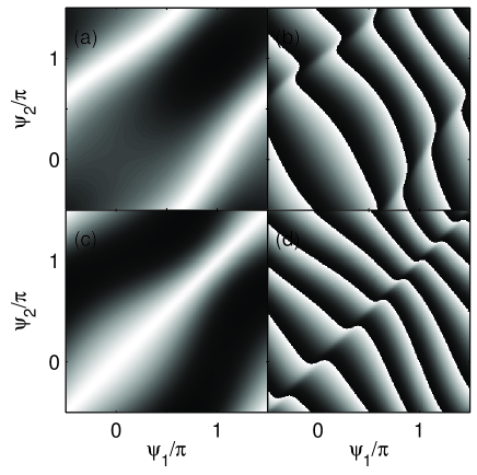
The highest energies for a given number of particles are achieved by putting almost all excitation into one mode, with the other two modes having very low excitation. Classically, these two modes have similar effective frequencies, (see Eq. (23)), and therefore they are locked easily. In Fig. 6 we show as examples the densities and phases for the states ${\Phi}_{461}$ and ${\Phi}_{433}$. In part (a) we see the density concentrated along the line $\psi_{1}=0$; thus, the transverse excitation number is $\mu_{t}=0$. Along this line, the phase function is almost like a plane wave. The total phase advance along one cycle around the organization center is $26\cdot 2\pi$. Accordingly, the longitudinal excitation number is $\mu_{l}=26$. Note that the phase function has singular points far away from the places of high density. In part (c) of the figure, we see the density concentrated along four lines in the $\psi_{2}$ direction. The four density crests are separated by 3 nodal lines, which can be seen very clearly as lines of discontinuities in the phase plot in part (d). Accordingly, the transverse excitation number of state ${\Phi}_{433}$ is $\mu_{t}=3$. Along the density crests we count the total phase advance to obtain the longitudinal quantum number $\mu_{l}=24$.

Figure 6: Plot of the eigenfunctions ${\Phi}_{461}$ and ${\Phi}_{433}$ of the quantum system belonging to the $\psi_{1}=0$ guiding center. Plot (a) shows $|{\Phi}_{461}|^{2}$, (b) shows $\arg({\Phi}_{461})\,\text{mod}\,2\pi$, (c) shows $|{\Phi}_{433}|^{2}$, (d) $\arg({\Phi}_{433})\,\text{mod}\,2\pi$. In the phase plots, the degree of darkness from white to black indicates the phase advance from $0$ to $2\pi$.

The energy distance between two states which differ by one unit in $\mu_{l}$ and that have the same transverse quantum number is given by the frequency of the classical organizing center, the periodic orbit (central fiber in the quasiperiodic motion shown in Fig. 3(b)), taken at an intermediate energy.

The classical motion behind this class of states is as follows: Mode 3 runs with its own effective frequency independently of the other modes. The quantum number $\mu_{l}$ is its action due to the semiclassical assignment of the phase function $\eta(\psi_{1},\psi_{2})$ to the classical action integral,

$$\eta(\psi_{1},\psi_{2})=\int\limits_{\gamma}\vec{J}\cdot d\vec{\psi}\,,$$ (28)

with $\vec{J}=(J_{1},J_{2})$ and $\vec{\psi}=(\psi_{1},\psi_{2})$. The phase $\eta(\psi_{1},\psi_{2})$ is defined by ${\Phi}=|{\Phi}|\exp\{i\eta\}$ and $\gamma$ is the classical guiding center. The path $\gamma$ is simply the line $\psi_{1}=0$ for this class and the the number of particles in mode 3 can be directly assigned to the quantum number $\mu_{l}$. Modes 1 and 2 run locked with total excitation, i. e. number of particles, $N-\mu_{l}$, and the quantum number $\mu_{t}$ characterizes the fluctuations of the coupled motion around the coupling point.

The eigenfunctions in this class can therefore be written approximately as

$${\Phi}_{\mu_{l},\mu_{t}}(\psi_{1},\psi_{2})\approx e^{iN\vartheta}\,e^{i\mu_{l}\psi_{2}}\,\chi_{\mu_{t}}(\psi_{1})\,.$$ (29)

Now we transform this expression back to the original coordinates, where we can interpret the actions $I_{k}$ directly as the number of particles in the potential well $k$. Using again transformation (12), we can write the idealized wave functions of this class as

$${\Phi}_{\mu_{l},\mu_{t}}(\varphi_{1},\varphi_{2},\varphi_{3})\\ \approx e^{i\mu_{l}\varphi_{3}}\,e^{i(N-\mu_{l})\varphi_{2}}\,\chi_{\mu_{t}}(\varphi_{1}-\varphi_{2})\,.$$ (30)

This type of wave function shows entanglement between modes 1 and 2, while mode 3 separates. The number of particles in mode 3 is given by $\mu_{l}$ while the transversal quantum number $\mu_{t}$ describes the transversal excitation of the organization center. A total of 51 eigenstates can be assigned to this class of functions.

Organization center $\bm{\psi_{2}=0}$ (Type (B))

The states of this class look very similar to those in the previous subsection, only with the roles of the modes 1 and 3 interchanged and hence with $\psi_{1}$ and $\psi_{2}$ interchanged. However, there is no perfect symmetry between classes C and B because there is no perfect equality between the modes 1 and 3. Remember that $\omega_{1}=-\omega_{3}\neq\omega_{3}$. This small perturbation of the symmetry is responsible that the states of class B loose their characteristics under smaller transverse excitations as the ones for class C. Accordingly we can assign less states to class B, namely 42 only, than we have assigned to class C.

Organization center $\bm{\psi_{1}=\psi_{2}}$ (Type (D))

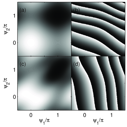
If almost all the action $K$ is in mode 2, then modes 1 and 3 have low actions and similar effective frequencies, whereas mode 2 has a quite different effective frequency. Even though the Hamiltonian does not contain a direct coupling between modes 1 and 3, sometimes the small indirect coupling is sufficient to cause locking between modes 1 and 3. Fig. 7 shows the states ${\Phi}_{420}$ and ${\Phi}_{359}$ as two examples of semiclassical wave functions in this class. The organization center is the diagonal $\psi_{1}=\psi_{2}$. State ${\Phi}_{420}$ has the transverse quantum number $\mu_{t}=0$ relative to this center and state ${\Phi}_{359}$ has $\mu_{t}=1$. The phase functions show that $\mu_{l}=6$ for state ${\Phi}_{420}$ and $\mu_{l}=8$ for state ${\Phi}_{420}$. The energy distance between two states, which differ by one unit in $\mu_{l}$ and that have the same transverse quantum number, is given by the frequency of the classical organizing center, namely the periodic orbit shown in Fig. 3(c) taken at an intermediate energy.

The classical motion carrying these states is the following: The coupled motion of modes 1 and 3 has the number of particles $\mu_{l}$ while the rest of the total excitation $N-\mu_{l}$ is in mode 2. The transverse quantum number $\mu_{t}$ again characterizes the fluctuations around the coupling point. For the idealized wave functions of the reduced system, we obtain

$${\Phi}_{\mu_{l},\mu_{t}}(\psi_{1},\psi_{2})\approx e^{iN\vartheta}\,e^{i\mu_{l}(\psi_{1}+\psi_{2})/2}\,\chi_{\mu_{t}}(\psi_{1}-\psi_{2})\,.$$ (31)

In the original coordinates, the wave function has the form

$${\Phi}_{\mu_{l},\mu_{t}}(\varphi_{1},\varphi_{2},\varphi_{3})\\ \approx e^{i(N-\mu_{l})\varphi_{2}}\,e^{i\mu_{l}(\varphi_{1}+\varphi_{3})/2}\,\chi_{\mu_{t}}(\varphi_{1}-\varphi_{3})\,.$$ (32)

In these coordinates, mode 2 separates from the other modes which are entangled. The number of particles in mode 2 is given by $N-\mu_{l}$, while the rest of the particles is in the entangled state of the other two modes, for which the quantum number $\mu_{t}$ is a measure of the fluctuations around the organization center. We can assign 8 eigenstates to this class of functions.

Figure 7: Plot of the eigenfunctions ${\Phi}_{420}$ and ${\Phi}_{359}$ of the quantum system belonging to the $\psi_{1}=\psi_{2}$ guiding center. Plot (a) shows $|{\Phi}_{420}|^{2}$, (b) $\arg({\Phi}_{420})\,\text{mod}\,2\pi$, (c) shows $|{\Phi}_{359}|^{2}$, (d) $\arg({\Phi}_{359})\,\text{mod}\,2\pi$.

Organization center $\bm{T^{2}}$ (Type (A))

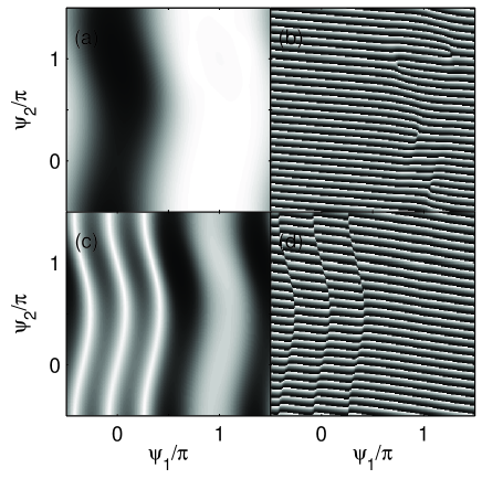
Fig. 8 shows the wave functions of the states ${\Phi}_{401}$ and ${\Phi}_{442}$, which do not show any coupling. These states belong to normal mode motion in the original modes. This does not necessarily mean that they have a constant density, but the density is without any clear structure and the phase function is close to a plane wave globally. As the two quantum numbers we count the phase advances around the two fundamental cycles of the toroidal configuration space. In part (b) of the figure we assign the quantum numbers $\mu_{l1}=2$, $\mu_{l2}=5$ and from part (d) we read off $\mu_{l1}=4$ and $\mu_{l2}=1$.

These states are described by the classical motion in the following way: The original mode 1 has the number of particles $\mu_{l1}$ and original mode 3 has $\mu_{l2}$ particles. The rest of the excitation $N-\mu_{l1}-\mu_{l2}$ is in mode 2. All three modes run independently with their own effective frequency. Thus phase functions of states of this class come close to a basis function (i.e. they resemble a plane wave), even though the wave function can be a strong mixture of several basis functions. The functional form of such states is therefore approximately given by

$${\Phi}_{\mu_{l1},\mu_{l2}}(\psi_{1},\psi_{2})\approx e^{iN\vartheta}\,e^{i(\mu_{l1}\psi_{1}+\mu_{l2}\psi_{2})}\,,$$ (33)

or written in the original coordinates as

$${\Phi}_{\mu_{l1},\mu_{l2}}(\varphi_{1},\varphi_{2},\varphi_{3})\approx e^{i\mu_{l1}\varphi_{1}}\,e^{i(N-\mu_{l1}-\mu_{l2})\varphi_{2}}\,e^{i\mu_{l2}\varphi_{3}}\,.$$ (34)

These idealized functions factorize and the three degrees of freedom are completely disentangled. There are 50 eigenstates in this class.

Figure 8: Plot of the eigenfunctions ${\Phi}_{401}$ and ${\Phi}_{442}$ of the quantum system belonging to the $T^{2}$ guiding center. Plot (a) shows $|{\Phi}_{401}|^{2}$, (b) $\arg({\Phi}_{401})\,\text{mod}\,2\pi$, (c) $|{\Phi}_{442}|^{2}$, (d) $\arg({\Phi}_{442})\,\text{mod}\,2\pi$.

States based on chaotic motion (Type (E2))

Finally, we give two examples of wave functions where we could not make any assignment to one of the organizing centers listed in the previous section. Fig. 9 shows the densities and phases of states ${\Phi}_{100}$ and ${\Phi}_{146}$. Neither in the density plots nor in the phase plots, can we discover any clean pattern related to one of the organizing centers. The connection to the classical motion we interpret as follows: In classical chaos, any typical trajectory jumps around irregularly between the neighborhoods of various simple periodic orbits and therefore between various types of motion. The corresponding quantum wave function should be random interference patterns of the structures belonging to the various organizing centers involved in the classical chaotic motion. Sometimes we can demix these interference patterns by forming appropriate linear combinations of several eigenfunctions of the Hamiltonian.

Figure 9: Plot of the eigenfunctions ${\Phi}_{100}$ and ${\Phi}_{146}$ of the quantum system belonging to class (E2). Plot (a) shows $|{\Phi}_{100}|^{2}$, (b) $\arg({\Phi}_{100})\,\text{mod}\,2\pi$, (c) shows $|{\Phi}_{146}|^{2}$, (d) $\arg({\Phi}_{146})\,\text{mod}\,2\pi$.

Concluding this section, we are able to characterize 180 of the 496 eigenstates within the scheme of guiding centers given by the classical motion (excluding chaotic motion). Our aim is not a complete assignment of all states, but rather to give an easy visual criterion in order to select states with different types of e.g. entanglement and localization properties as described in this section for each class. For these states, one can use the classical picture in order to understand the quantum mechanical structure, which allows a very intuitive treatment of the states. The above graphical classification of the semiclassical wave functions is not strict and some functions allow ambiguous assignments. Such functions show characteristics of different classes and it is only a matter of degree in which class to put them. For example, the phase functions in Fig. 7 could be interpreted as continuous deformations of plane waves and therefore they could be assigned to type (A) as well.

V Comparison of the time dynamics

Finally, we wish to discuss the implications of our analysis for the time evolution in the classical description of the system. The classical system can be interpreted as an array of three Bose-Einstein condensates where the condensate in each well is described by the Gross-Pitaevskii equation and where the condensates interact weekly through Josephson tunneling Smer97 ; Milb97 .

In the previous section, we have used the classical system only to provide a tool for the classification of the quantum wave functions, and we have shown how close the quantum eigenfunctions resemble the classical guiding centers. In this section, we look in the other direction. Starting from the classical system, i.e. the mean-field equations, we want to ask what information the structure of the quantum system can provide in order to solve the mean-field equations: the analysis of a system of coupled nonlinear differential equations is very involved, while in the quantum system we only have to diagonalize the Hamiltonian numerically and plot the eigenfunctions in configuration space.

Since it is more convenient in this context to speak about complex occupation amplitudes, we introduce the new variables

$$c_{k}=\sqrt{I_{k}}\,e^{i\varphi_{k}}\,.$$ (35)

In these variables, the classical Hamiltonian (II.1) can be written as

$$H =\sum_{k=1}^{3}\bigl{(}\,\omega_{k}|c_{k}|^{2}+x_{k}|c_{k}|^{4}\,\bigr{)}$$

$$\quad-\frac{k_{12}}{2}(c_{1}c_{2}^{*}+c_{2}c_{1}^{*})-\frac{k_{23}}{2}(c_{2}c_{3}^{*}+c_{3}c_{2}^{*})\,,$$ (36)

with canonically conjugate variables $(c_{k},ic_{k}^{*})$ and corresponding equations of motion

$$\dot{c}_{k}=\frac{\partial H}{\partial(ic_{k}^{*})}\quad\Longleftrightarrow\quad i\,\dot{c}_{k}^{*}=\frac{\partial H}{\partial c_{k}}\;.$$ (37)

This system of three ordinary differential equations for the complex coefficients $c_{k}$ is equivalent to the six equations for the angles $\varphi_{k}$ and the actions $I_{k}$ with $k=1,2,3$. The equations can also be derived from the Gross-Pitaevskii equation in coordinate space using an expansion of the condensate wave function in Wannier functions Trom01 . One can also use the eigenstates of the one-particle Hamiltonian, the so-called Wannier-Stark functions, resulting in the disappearance of the linear tunneling terms in the Hamiltonian (3), while higher order coupling terms become important Thom03 .

Now we choose the initial conditions $c_{k}(t=0)$ by using the semiclassical correspondence (7) between the classical actions $I_{k}$ and the quantum numbers $n_{k}$ of a number state $|n_{1},n_{2},n_{3}\rangle$:

$$I_{k}\longleftrightarrow n_{k}+\frac{1}{2}\,.$$ (38)

In this way, we can construct initial conditions $c_{k}(0)=\sqrt{I_{k}}$, where the action $I_{k}$ can be interpreted quantum mechanically via Eq. (38) as the number of particles in mode $k$. Furthermore, we can use this correspondence in order to construct initial conditions resembling the properties of the eigenstates of the system. Before we explain this in more detail we first discuss the case of the basis vectors.

V.1 Basis vectors

Here we investigate to which extend we can attribute the same characteristics to the quantum mechanical number states $|n_{1},n_{2},n_{3}\rangle$ and their classical analog defined by Eq. (38). Accordingly, we define the initial conditions for the time evolution of Eq. (37) as

$$\vec{b}(t=0;n_{1},n_{2},n_{3})=(c_{1}(0),c_{2}(0),c_{3}(0))=$$

$$\quad=(\sqrt{n_{1}+1/2},\sqrt{n_{2}+1/2},\sqrt{n_{3}+1/2})\,.$$ (39)

In the following we will not explicitly write down the dependence of $\vec{b}(t;n_{1},n_{2},n_{3})$ on the initial condition through the parameters $(n_{1},n_{2},n_{3})$ and simply use $b(t)$. We fix the three initial phases to zero, which corresponds to zero imaginary part of the $c_{k}(0)$. With this initial conditions the time evolution can be calculated numerically, as shown in

Figure 10: (Color online) Time evolution of Eq. (37) for an initial condition $\vec{b}(0)=(\sqrt{2.5},\sqrt{5.5},\sqrt{23.5})$. Shown are squared modulus (top) and the phase of the first (solid, black), second (dashed, green) and third (dash-dotted, red) mode. In the phase plot the first and second phase almost coincide and lie above the third phase which has a bigger phase velocity. The time is measured with respect to $T=2\pi/\omega$.

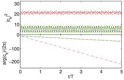
Fig. 10 for initial values $(\sqrt{2.5},\sqrt{5.5},\sqrt{23.5})$ using Eq. (37). In this example the phases of $c_{1}$ and $c_{2}$ are locked, while $c_{3}$ evolves independently. The difference in the amplitudes between mode 3 and the other two prohibits a coupling. The amplitudes show a quite regular oscillation in all three modes. This is motion of type (C) introduced in section III. Physically interpreted, the wells 1 and 2 couple through Josephson tunneling and the population between the two wells is exchanged periodically. In contrast, the number of particles of well 3 stays approximately constant and much higher than the population of the other wells. This behavior reflects the well-known macroscopic self-trapping found in the double well potential Smer97 . Another type of this self-trapping effect in the type (C) dynamics can occur, when wells 1 and 2 have approximately the same population $N/2$ and well 3 is nearly empty. One can also observe the other types of dynamics in the vectors $\vec{b}(t)$, except type (D), due to the very weak indirect coupling between modes 1 and 3. The different time evolutions $\vec{b}(t)$ can be easily assigned to the different guiding centers by looking at the phases:

Figure 11: (Color online) Time evolution for an initial condition $\vec{b}(t=0)=(\sqrt{23.5},\sqrt{7.5},\sqrt{0.5})$. Shown are squared modulus (top) and the phase of the first (solid, black), second (dashed, green) and third (dash-dotted, red) mode. The time is measured with respect to $T=2\pi/\omega$.

Type (A): All three phases behave independently and the amplitudes oscillate regularly. The individual condensates in the different wells are completely decoupled and the population in each well stays approximately constant.

Type (B): The dynamics shows the same behavior as for type (C), but with phase locking between mode 2 and 3.

Type (D): This type of motion is difficult to identify, because the indirect phase locking between modes 1 and 3 is very weak. This leads to the effect that the phase velocities of these two phases are very close, but still distinguishable. This is of course not a strict statement, and it depends on how long the time propagation is considered. The problems with the classification of this type can also be seen in the quantum case in Fig. 7. In parts (b) resp. (d), the phase singularities are not sharp but rather smooth, so these states could be assigned to type (A) as well.

Type (E1): In this case all three phases evolve with the same velocity and the amplitudes show similar regular oscillations as in types (B) and (C) for two locked phases.

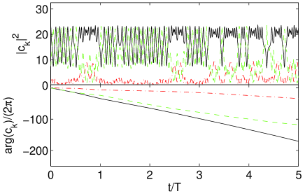
Type (E2): This class is characterized by intermittencies as illustrated in Fig. 11. The dynamics can be interpreted in such a way that the trajectories jump irregularly between different coupling schemes. Accordingly, frequency locking between different pairs of modes is only established temporarily during the time evolution.

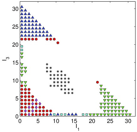
With this scheme, we can classify the dynamics of all possible basis states $\vec{b}(t)$, as shown in Fig. 12. The interesting point is that we can compare these results with the information that we extract from the semiclassical wave functions. For this we compare for a given basis state $|n_{1},n_{2},n_{3}\rangle$ all eigenfunctions (22) to which the basis state contributes significantly and assign a type (A)–(E2) to this basis state if possible. The result is shown in Fig. 13.

Figure 12: (Color online) Characterization of the classical actions $I_{k}=|c_{k}|^{2}$ through direct numerical integration of Eq. (37). The action $I_{2}$ is given by $I_{2}=K-I_{1}-I_{3}$. Plotted are time evolutions of type (A) ($\circ$, red), type (B) ($\triangledown$, green), type (C) ($\triangle$, blue), type (E1) ($*$, black) and type (E2) ($\square$, cyan).

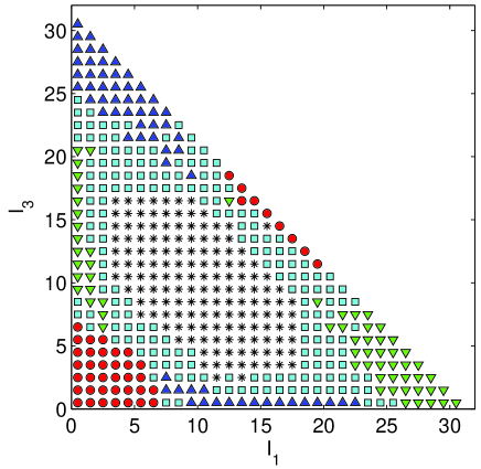
The points with no symbol indicate states which cannot be assigned uniquely to a certain type. However, for the shown basis states one can see a close correspondence between the classical and the quantum system. Only at the fringes are there small deviations. Therefore the quantum mechanical analysis provides a grid of initial conditions for which we can predict the behavior of the solutions of the mean-field equations. Finally, we remark, that the classification of the basis states in Fig. 12 holds in principle also for an arbitrary choice of the initial phases in Eq. (V.1). Only at the fringes of the different zones does the behavior of the time dynamics depend crucially on the initial conditions and there it can deviate from this classification.

Figure 13: (Color online) Characterization of the classical actions $I_{k}=|c_{k}|^{2}$ through the semiclassical wave functions. The action $I_{2}$ is given by $I_{2}=K-I_{1}-I_{3}$. Plotted are actions whose quantum analog belongs to type (A) ($\circ$, red), type (B) ($\triangledown$, green), type (C) ($\triangle$, blue), type (D) ($\diamond$, magenta), type (E1) (*, black), and type (E2) ($\square$, cyan).

V.2 Eigenstates

In the last section we discussed the close resemblance between the quantum and the classical picture by assigning the same characterization scheme with types (A)–(E2) to the basis functions and the solutions of the mean-field equations. In this section we want to investigate, whether also the eigenstates of the quantum system can be reinterpreted classically, i. e. if they can be used to identify the different types of dynamical behavior in the system of the three Bose-Einstein condensates weakly coupled by Josephson junctions. We construct the classical analog of Eq. (21) by defining the set of vectors

$$\vec{B}(n_{1},n_{2},n_{3})=(n_{1}+1/2,n_{2}+1/2,n_{3}+1/2)\,,$$ (40)

which are related to the vectors $\vec{b}(t=0)$ by $B_{k}=b_{k}^{2}(0)$ (cf. Eq. (V.1)). However, note that the vectors $\vec{B}(n_{1},n_{2},n_{3})$, like the vectors $\vec{b}(t;n_{1},n_{2},n_{3})$ of Eq. (V.1), do not form a basis of ${\mathbb{C}}^{3}$. In analogy to Eq. (20) one can write

$$\vec{{\Phi}}(t=0)=\!\!\!\!\!\!\!\sum_{n_{1}+n_{2}+n_{3}=N}\!\!\!\!\!\!\!c_{n_{1},n_{2},n_{3}}^{2}\,\vec{B}(n_{1},n_{2},n_{3})\,,$$ (41)

where the real-valued coefficients $c_{n_{1},n_{2},n_{3}}$ are taken from Eq. (21).

Figure 14: (Color online) Time evolution of the mean-field equations for an initial condition corresponding to the first quantum eigenstate. Shown are squared modulus (top) and the phase of the first ($-$, black), second ($--$, green) and third ($-\cdot-$, red) mode. The time is measured with respect to $T=2\pi/\omega$.

In this naive approach, the vector $\vec{{\Phi}}$ can be interpreted as the quantum expectation value of the action $\hat{\vec{I}}$ ($\hat{I}_{k}=\hat{n}_{k}+1/2$) in the quantum state $|{\Phi}\rangle$,

$$\langle{\Phi}|\hat{I}_{k}|{\Phi}\rangle=\sum_{n_{1},n_{2},n_{3}}c_{n_{1},n_{2},n_{3}}^{2}\,(n_{k}+{1}/{2})\,,$$ (42)

where we have simply used the representation (20) of the eigenfunctions. The initial phases are chosen equal zero like in the case of the basis vectors. In order to use this vector $\vec{{\Phi}}$ as initial conditions for the mean-field equations, we must take the square root of each component, and to this end we define the new vector $\vec{\phi}$ with components $\phi_{k}=\sqrt{\Phi_{k}}$. These vectors are normalized as

$$|\vec{\phi}|^{2}=\sum_{k=1}^{3}\Phi_{k}=\!\!\!\!\!\!\!\sum_{n_{1}+n_{2}+n_{3}=N}\!\!\!\!\!\!\!c_{n_{1},n_{2},n_{3}}^{2}\,\sum_{k=1}^{3}B_{k}=K\,,$$ (43)

where $K=31.5=N+3/2$ is the classically conserved total action of Eq. (10). In the context of the Gross-Pitaevskii equation, the norm of the condensate wave function gives the number of particles in the condensate. We get the additional term of $3/2$ for the number of particles compared to the many-particle Hamiltonian (3), since we use the semiclassical correspondence of Eq. (7). For Bose-Einstein condensates with a number of particles much larger than $30$, one can ignore the term $1/2$ in Eq. (7) and obtain the standard correspondence between the particle numbers. However, for $N=30$, semiclassical studies like the present work show that the identification (7) gives a much better agreement between classical and quantum mechanics. In order to obtain the normalization $|\vec{\phi^{\prime}}|^{2}=1$, one simply has to set $\vec{\phi}=\vec{\phi^{\prime}}\sqrt{N}$ and replace the nonlinearities $x_{k}$ by $x_{k}=g/K$.

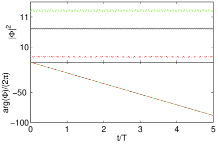
In Fig. 14, the time evolution for the initial condition $\vec{{\Phi}}_{1}$ is shown. The time evolution shows approximately constant occupations $|c_{k}|^{2}$ (upper panel), and the three phases are locked. In the reduced system, this corresponds to a point in the neighborhood of a fixed point. For the parameter values chosen in this article, there does not exist an exact fixed point of the Hamiltonian flow of the reduced system, although this point serves as guiding center for the wave functions of type (E1). In that sense the semiclassical wave functions behave very similarly in the neighborhood of a guiding center, while the solutions of the Gross-Pitaevskii equation are very sensitive to small deviations due to the nonlinearity of the time-evolution.

Another example is shown in Fig. 15 for a type (A) motion.

Figure 15: (Color online) Time evolution of Eq. (37) for the initial condition ${\Phi}_{444}(0)$. Shown are squared modulus (top) and the phase of the first ($-$, black), second ($--$, green) and third ($-\cdot-$, red) mode. The time is measured with respect to $T=2\pi/\omega$.

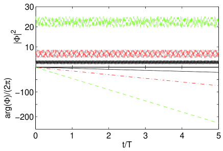
The phases of the modes evolve independently and the amplitudes show tiny oscillations, due to the fact that the time evolution does not coincide with the corresponding idealized guiding center of type (A). Because the system is dominated by the anharmonicities the effective frequencies are almost linear in the actions according to Eq. (23). Therefore the slopes of the phase curves are proportional to the average values of the corresponding actions.

To conclude, from the classical point of view the analysis of the corresponding quantum system offers a direct visual method for the understanding of the structure and can be used to identify the dynamical behavior of the system of the three weakly coupled Bose-Einstein condensates in the mean-field approximation simply by diagonalizing the quantum Hamiltonian and plotting the eigenfunctions in the appropriate basis.

VI Conclusion

In our investigation of a Bose-Einstein condensate in a multi-well potential, we showed a close correspondence between the quantum mechanical description and a classical version where the bosonic creation and annihilation operators of the many particle system are replaced by c-numbers. We truncated the many-particle Hamiltonian to a few relevant modes and obtained a system of three coupled anharmonic oscillators. Whether the truncation at a small number of modes is justified depends crucially on an appropriate choice of the expansion basis and on the external potential. In order to compare the quantum system with its classical counterpart, we introduced the concept of the semiclassical wave functions defined on the same toroidal configuration space as in the classical system. This choice of the quantum mechanical representation allowed us to compare the quantum system directly with the classical system. In both cases, for the classical and the quantum system, we used the conserved particle number resp. total action to reduce the degrees of freedom to two. Classically, we can identify various geometric structures in phase space that are connected to different types of motion in the configuration space. These different types of motion belonging to the various guiding centers, are also found in the quantum mechanical wave functions. So we used these guiding centers firstly to sort a large number of wave function into these different classes, and secondly to assign uniquely geometric quantum numbers to the wave functions within one class. In this geometric picture, the wave functions describe the quantum excitations of the underlying classical dynamics. As an application, we can characterize the entanglement between the different modes and we can also determine the number of particles in each of the entangled modes using their associated quantum numbers.

In the last part of this article we analyzed the significance of the quantum mechanical classification of the wave functions for the classical dynamics. For this we studied classical trajectories which have initial conditions corresponding to quantum mechanical number states, or which correspond to the eigenstates directly. In both cases, we could obtain the characteristics of the semiclassical classification also from the classical trajectories, although the classical dynamics is much more sensitive to deviations from the idealized guiding centers.

Concluding, we showed that semiclassical wave functions provide an intuitive picture of the quantum mechanical many-particle eigenfunctions, and allow a direct classification of the dynamics.

References

- (1) M. Albiez, R. Gati, J. Fölling, S. Hunsmann, M. Cristiani and M. K. Oberthaler, Phys. Rev. Lett. 95 (2005) 010402
- (2) T. Schumm, S. Hofferberth, L. M. Andersson, S. Wildermuth, S. Groth, I. Bar-Joseph, J. Schmiedmayer and P. Krüger, Nature Physics 1 (2005) 57
- (3) A. Smerzi, S. Fantoni, S. Giovanazzi, and S. R. Shenoy, Phys. Rev. Lett. 79 (1997) 4950
- (4) D. Witthaut, E. M. Graefe, and H. J. Korsch, Phys. Rev. A 73 (2006) 063609
- (5) J. Liu, B. Wu, and Q. Niu, Phys. Rev. Lett. 90 (2003) 170404
- (6) Biao Wu and Qian Niu, New J. Phys. 5 (2003) 104
- (7) G. J. Milburn, J. Corney, E. M. Wright, and D. F. Walls, Phys. Rev. A 55 (1997) 4318
- (8) A. Smerzi and Srikanth Raghavan, Phys. Rev. A 61 (2000) 063601
- (9) J. R. Anglin and A.Vardi, Phys. Rev. A 64 (2001) 013605
- (10) J. R. Anglin, P. Drummond and A. Smerzi, Phys. Rev. A 64 (2001) 063605
- (11) Q. Thommen, J. C. Garreau, and V. Zehnlé, Phys. Rev. Lett. 91 (2003) 210405
- (12) K. W. Mahmud, H. Perry and W. P. Reinhardt, Phys. Rev. A 71 (2005) 023615
- (13) E. L. Sibert III and A. B. McCoy, J. Chem. Phys. 105 (1996) 469
- (14) M. P. Jacobson, C. Jung, H. S. Taylor, and R. W. Field, J. Chem. Phys. 111 (1999) 600
- (15) C. Jung, H. S. Taylor and E. Atilgan, J. Phys. Chem. A 106 (2002) 3092
- (16) C. Jung, C. Mejia-Monasterio, and H. S. Taylor, J. Chem. Phys. 120 (2004) 4194
- (17) E. M. Graefe, H. J. Korsch, and D. Witthaut, Phys. Rev. A 73 (2006) 013617
- (18) K. Nemoto, C. A. Holmes, G. J. Milburn and W. J. Munro, Phys. Rev. A 63 (2000) 013604
- (19) P. Buonsante, R. Franzosi and V. Penna, Phys. Rev. Lett. 90 (2003) 050404
- (20) R. Franzosi and V. Penna, Phys. Rev. E 67 (2003) 046227
- (21) P. Buonsante, R. Franzosi and V. Penna, J. Phys. B 37 (2004) S229
- (22) W. Kohn, Phys. Rev. 115 (1959) 809
- (23) M. P. A. Fisher, P. B. Weichman, G. Grinstein, and D. S. Fisher, Phys. Rev. B 40 (1989) 546
- (24) R.W. Spekkens and J.E. Sipe, Phys. Rev. A 59 (1999) 3868
- (25) W. Heisenberg, Z. Physik 33 (1925) 879
- (26) M. Brack and R. K. Bhaduri, Semiclassical physics, Addison Wesley, 1997
- (27) M. C. Gutzwiller, Chaos in Classical and Quantum Mechanics, Springer, New York, 1990
- (28) B. V. Chirikov, Phys. Rep. 52 (1979) 263
- (29) R. Jost, M. Joyeux, S. Skokov and J. Bowman, J. Chem. Phys. 111 (1999) 6807
- (30) T. Azzam, R. Schinke, S. Farantos, M. Joyeux and K. Peterson, J. Chem. Phys. 118 (2003) 9643
- (31) J. Gomez Llorente, J. Zakrzewski and H. S. Taylor, J. Chem. Phys. 90 (1989) 1505
- (32) A. Trombettoni and A. Smerzi, Phys. Rev. Lett. 86 (2001) 2353