Ghost imaging with intense fields from chaotically-seeded parametric downconversion

Emiliano Puddu and Alessandra Andreoni

Dipartimento di Fisica e Matematica, Università degli Studi dell’Insubria,
Istituto Nazionale per la Fisica della Materia (C.N.R-I.N.F.M.), Como, Italy

Ivo Pietro Degiovanni

Istituto Nazionale di Ricerca Metrologica, Torino, Italy

Maria Bondani

National Laboratory for Ultrafast and Ultraintense Optical Science, C.N.R.-I.N.F.M., Como, Italy

Stefania Castelletto

Physics School, Melbourne University, Victoria, Australia

Abstract

We present the first experimental demonstration of ghost imaging realized with intense beams generated by a parametric down conversion interaction seeded with pseudo-thermal light. As expected, the real image of the object is reconstructed satisfying the thin-lens equation. We show that the experimental visibility of the reconstructed image is in accordance with the theoretically expected one.

OCIS codes: 270.0270, 190.2620, 270.5290, 030.0030, 100.0100

Ghost imaging capability was initially attributed only to entangled photon pairs,[1] but in more recent works it has been ascertained also for classically correlated fields, both in the single photon regime [2, 3] and in the continuous variable regime.[4] The main result of all these schemes is the non-local imaging of objects both in near- and far-field. [5] A general ghost-imaging scheme involves a source of correlated bipartite field and two propagation arms usually called Test (T) and Reference (R). In the T-arm the object to be imaged is inserted and a bucket (or a pointlike) detector measures the light transmitted by the object. The R-arm contains an optical setup suitable for reconstructing the image of the object (or its Fourier transform) and a position-sensitive detector.
In this Letter we show a ghost imaging experiment performed by using the intense fields generated by parametric downconversion (PDC) seeded with multimode chaotic light. As usual in ghost imaging experiments, the technique adopted for the retrieval of the image consists in the evaluation of the fourth-order correlation between the fields at the detection planes.
In Fig. 1 we show our experimental setup. We injected a coherent collimated pump beam ($\lambda_{P}=532$ nm) and a seed beam ($\lambda=1064$ nm) into a crystal of $\beta$-BaB₂O₄ (BBO, cut angle 22.8 $\deg$, 10 mm$\times$10 mm$\times$3 mm, Fujian Castech Crystals) in type-I interaction geometry. Both pump and seed beams were provided by an amplified Q-switched Nd:YAG laser (GCR-4, 10 Hz repetition rate, 7 ns pulse duration of the fundamental pulse, Spectra-Physics). The seed field was randomized by passing it through two independently rotating ground glass plates, [6] P₁ and P₂ in order to obtain a pseudo-thermal statistics. The speckles on the object plane resulted to be about 320 $\mu$m in diameter as evaluated by spatial autocorrelation. The object was a hole of 1.6 mm diameter crossed by a straight wire of 0.5 mm caliber. As the D_T and D_R detectors, we used a single CCD camera (CA-D1-256T, 16 $\mu$m$\times$16 $\mu$m pixel area, 12 bit resolution, Dalsa). The CCD sensor, also depicted in Fig. 1, for one half recorded the single-shot intensity Maps in the R-arm, $\mathcal{I}_{R}(\mathbf{x}_{R})$, and for the other half realized the bucket detector of the T-arm.

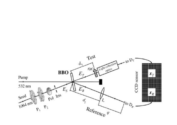
Fig. 1: Experimental setup: P_1,2, independently rotating ground glass plates: Pol, polarizer; $t(\mathbf{x})$, object transmission function; L, lens; tuning angle 24.7 deg.

In the following, $\mathcal{I}_{T}$ designates the sum of the contents of $110\times 110$ pixels of D_T in a single shot. The T-arm includes free propagation over $d_{1}=60$ cm from BBO to object, transmission function $t(\mathbf{x})$, and light collection optics in front of $D_{T}$. The R-arm contains free propagation over $d_{2}=60$ cm from BBO to lens L ($f=400$ mm) and from L to the CCD camera ($q=60$ cm). Distances $d_{1}$, $d_{2}$ and $q$ and focal length $f$ must satisfy $1/(d_{1}+d_{2})+1/q=1/f$ to give an imaging system with magnification factor $M=q/(d_{1}+d_{2})$.[1]
The evolution of the system is described by the unitary operator $S$ generated by the multimode PDC hamiltonian [7] and the input-output relations that link the output operators $b_{i,\mathbf{q}}$ to the input operators $a_{i,\mathbf{q}}$ are

$$b_{i,\mathbf{q}}=S^{\dagger}a_{i,\mathbf{q}}S=U_{i,\mathbf{q}}a_{i,\mathbf{q}}+V_{i,\mathbf{q}}e^{i\varphi_{\mathbf{q}}}a^{\dagger}_{j,-\mathbf{q}}~{}~{}~{}~{}~{}~{}i=R,T;~{}i\neq j,$$ (1)

where $U_{i,\mathbf{q}}^{2}-V_{i,\mathbf{q}}^{2}=1$ and $\{U,V,\varphi\}_{\mathbf{q}}=\{U,V,\varphi\}_{-\mathbf{q}}$. We take $a_{R,\mathbf{q}}$ in the vacuum state and $a_{T,\mathbf{q}}$ in the multimode thermal state represented by the density matrix

$$\rho_{T}=\prod^{\otimes}_{\mathbf{q}}\left\{\sum_{m=0}^{\infty}p_{T,{\mathbf{q}}}(m)\left|m\right\rangle\left\langle m\right|_{T,{\mathbf{q}}}\right\}\;,$$ (2)

where $\left|m\right\rangle_{\mathbf{q}}$ is the Fock state with $m$ photons in mode $\mathbf{q}$ and $p_{T,{\mathbf{q}}}(m)=n_{th,\mathbf{q}}^{m}/(1+n_{th,\mathbf{q}})^{m+1}$ is the photon number distribution on the single mode for $n_{th,\mathbf{q}}$ mean photon number. The the output state is obtained by exploiting the Baker-Campbell-Hausdorff formula[7, 8]

$$\rho_{out}=S(\rho_{T}\otimes\left|0\right\rangle\left\langle 0\right|_{R})S^{\dagger}$$

$$\qquad=\prod^{\otimes}_{\mathbf{q}}\sum_{n}p_{T,{\mathbf{q}}}(n)\sum_{n_{1},n_{2}}F_{\mathbf{q}}(n,n_{1},n_{2})$$

$$\qquad\quad\left|n+n_{1}\right\rangle\left\langle n+n_{2}\right|_{T,{\mathbf{q}}}\otimes\left|n_{1}\right\rangle\left\langle n_{2}\right|_{T,-{\mathbf{q}}}$$ (3)

where we have defined

$$F_{\mathbf{q}}(n,n_{1},n_{2})=\frac{\left(n_{\mathrm{PDC},\mathbf{q}}\right)^{\frac{n_{1}+n_{2}}{2}}}{\left(1+n_{\mathrm{PDC},\mathbf{q}}\right)^{n+1+\frac{n_{1}+n_{2}}{2}}}$$

$$\qquad\qquad\qquad\times\sqrt{\frac{(n+n_{1})!}{n!n_{1}!}}\sqrt{\frac{(n+n_{2})!}{n!n_{2}!}}$$ (4)

$n_{\mathrm{PDC},\mathbf{q}}=V_{R,\mathbf{q}}^{2}$ being the mean photon number per mode generated by spontaneous PDC. The marginal distributions on $R$- and $T$-arms are multithermal.
By direct application of the Peres-Horodecki-Simon criterion[9, 10, 11] it can be demonstrated that the state $\rho_{out}$ is inseparable for any value of $n_{th,\mathbf{q}}$.[12]
The reconstruction of the image is achieved by the computation of the correlation function, $G^{(2)}(\mathbf{x}_{R})$. This procedure is equivalent first to evaluate the correlation function between $I_{R}(\mathbf{x}_{R})$ and $I_{T}(\mathbf{x}_{T})$

$$\mathcal{G}^{(2)}(\mathbf{x}_{R},\mathbf{x}_{T})=\langle I_{R}(\mathbf{x}_{R})I_{T}(\mathbf{x}_{T})\rangle-\langle I_{R}(\mathbf{x}_{R})\rangle\langle I_{T}(\mathbf{x}_{T})\rangle,$$ (5)

where $\langle I_{i}(\mathbf{x}_{i})\rangle=\langle c_{i}^{\dagger}(\mathbf{x}_{i})c_{i}(\mathbf{x}_{i})\rangle$ ($i=R,T$) is the mean intensity of the i-th beam and $\langle I_{R}(\mathbf{x}_{R})I_{T}(\mathbf{x}_{T})\rangle=\langle c_{R}^{\dagger}(\mathbf{x}_{R})c_{R}(\mathbf{x}_{R})c_{T}^{\dagger}(\mathbf{x}_{T})c_{T}(\mathbf{x}_{T})\rangle$ (where $\langle...\rangle=\mathrm{Tr}[...\rho_{T}\otimes\left|0\right\rangle\left\langle 0\right|_{R}]$), and then to perform the integration

$$G^{(2)}(\mathbf{x}_{R})=\int{d\mathbf{x}_{T}\mathcal{G}^{(2)}(\mathbf{x}_{R},\mathbf{x}_{T})}.$$ (6)

The propagation to $D_{R}$ and $D_{T}$ is described by the corresponding impulse response functions $h_{R}(\mathbf{x}_{R},\mathbf{x}_{R}^{\prime})$ and $h_{T}(\mathbf{x}_{T},\mathbf{x}_{T}^{\prime})$, whose derivation is straightforward, [13] and the field operators at the detection planes become $c_{i}(\mathbf{x}_{i})=\int{\rm d}\mathbf{x}_{i}^{\prime}h_{i}(\mathbf{x}_{i},\mathbf{x}_{i}^{\prime})b_{i}(\mathbf{x}_{i}^{\prime})$, where $b_{i}(\mathbf{x})\propto\sum_{\mathbf{q}}\exp(i\mathbf{q}\cdot\mathbf{x})b_{i,\mathbf{q}}$. The factorization rule for $\langle b_{R}^{\dagger}(\mathbf{x}_{R}^{\prime\prime})b_{R}(\mathbf{x}_{R}^{\prime})b_{T}^{\dagger}(\mathbf{x}_{T}^{\prime\prime})b_{T}(\mathbf{x}_{T}^{\prime})\rangle$ in this case is exactly the same as that for spontaneous PDC[14], thus in the degenerate case Eq. (5) becomes

$$\mathcal{G}^{(2)}(\mathbf{x}_{R},\mathbf{x}_{T})=$$

$$\left|\int{\rm d}\mathbf{x}_{R}^{\prime}\int{\rm d}\mathbf{x}_{T}^{\prime}h_{R}(\mathbf{x}_{R},\mathbf{x}_{R}^{\prime})h_{T}(\mathbf{x}_{T},\mathbf{x}_{T}^{\prime})\langle b_{R}(\mathbf{x}_{R}^{\prime})b_{T}(\mathbf{x}_{T}^{\prime})\rangle\right|^{2}.$$ (7)

If the coherence area of the multithermal field is much smaller than the object, we can proceed as in Ref. [14] and get

$$G^{(2)}(\mathbf{x}_{R})\propto\left|t(-M\mathbf{x}_{R})\right|^{2}\int{\rm d}\mathbf{x}_{T}n_{\mathrm{PDC}}\left(\frac{2\pi\mathbf{x}_{T}}{\lambda f}\right)$$

$$\times\left[1+n_{\mathrm{PDC}}\left(\frac{2\pi\mathbf{x}_{T}}{\lambda f}\right)\right]\left[1+n_{th}\left(\frac{2\pi\mathbf{x}_{T}}{\lambda f}\right)\right]^{2}.$$ (8)

In our experiment we estimate $n_{\mathrm{PDC}}\simeq 0.5$ and $n_{th}\simeq 10^{12}$ per spatial mode. The correlation function in Eq. (8) reproduces the object and depends on the properties of our source through the mean photon numbers of downconverted fields and of the chaotic seeding field.
The experimental results are shown in Fig. 2: panel a) displays a typical sample of chaotic intensity Map $\mathcal{I}_{R}(\mathbf{x}_{R})$ recorded in single shot, whereas panel b) contains the map of the correlation coefficients

$$C(\mathbf{x}_{R})=\frac{G^{(2)}(\mathbf{x}_{R})}{\sqrt{\sigma^{2}(I_{R}(\mathbf{x}_{R}))\sigma^{2}(I_{T})}}$$ (9)

evaluated over an ensemble of 9500 single shot Maps, where $\sigma^{2}(I)=\langle I^{2}\rangle-\langle I\rangle^{2}$ and both intensities and variances were evaluated by subtracting the statistical contributions of the background noise. To measure the noise we considered the values recorded by the CCD in a non-illuminated sensor region. Panel b) in Fig. 2 shows that the recovered image has the correct size, as compared to the original object, being $M=0.5$.

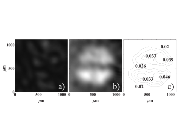
Fig. 2: a) Single-shot Map recorded in the R-arm; b) ghost image; c) contour plot of the local visibility.

To quantify the quality of our technique, we define the local visibility of the reconstructed image (see Ref.[15]) as

$$\mathcal{V}(\mathbf{x}_{R})=\frac{G^{(2)}(\mathbf{x}_{R})}{\langle I_{R}(\mathbf{x}_{R})I_{T}\rangle}=\frac{G^{(2)}(\mathbf{x}_{R})}{\langle I_{R}(\mathbf{x}_{R})\rangle\langle I_{T}\rangle+G^{(2)}(\mathbf{x}_{R})}$$ (10)

and evaluate it for the ghost image in Fig. 2 b). Figure 2 c) shows the contour plot of $\mathcal{V}(\mathbf{x}_{R})$ at the marked levels including the maximum value 0.046.

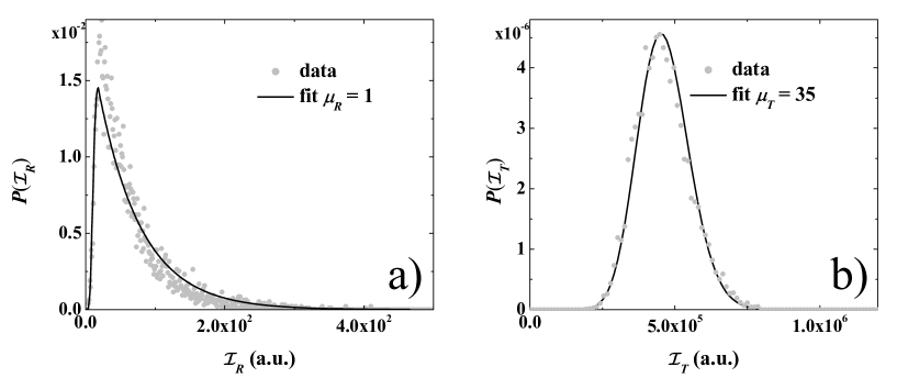
Fig. 3: a) Statistical distribution of the intensity in a single pixel of the $D_{R}$ detector (dots) and multithermal fit giving $\mu_{R}=1$ (full line); b) statistical distribution of the intensity on the bucket detector (dots) and multithermal fit giving $\mu_{T}=35$ (full line).

A tradeoff between visibility and resolution of the reconstructed image has been reported[15] that depends on the number of spatial modes (coherence areas, $A_{C}$) that illuminate an object of area $A_{O}$. In our case $A_{O}/A_{C}\simeq 1600^{2}/320^{2}=25$. This number being rather low, we observe a quite poor image resolution and a quite high visibility. To confirm our results we calculate the number of spatial and temporal modes, involved in the interaction. We start by studying the statistical distributions of the beam intensities detected either in a single pixel $\mathbf{x}_{R}$ or by the bucket detector in the T-arm. In Fig. 3 we show the experimental distributions along with the best fitting curves obtained by convolving the theoretical multithermal distribution[16, 7]

$$P_{\mu}(\mathcal{I})=\frac{e^{-\mu\mathcal{I}/\langle I\rangle}}{\left(\langle I\rangle/\mu\right)^{\mu}}\frac{\mathcal{I}^{\mu-1}}{\left(\mu-1\right)!}\>$$ (11)

with the experimental one obtained for the background. Here $\mathcal{I}$ indicates the single-shot values of either $\mathcal{I}_{R}(\mathbf{x}_{R})$ or $\mathcal{I}_{T}$, whose mean values and variances obviously coincide with those of the operators $I_{R}(\mathbf{x}_{R})$ and $I_{T}$. From the data in panel a) we obtained $\mu_{R}=1$, independently of the position $\mathbf{x}_{R}$ we tested, and from the data in panel b), $\mu_{T}=35$. As the statistical distribution in Fig. 3 a) reflects the behavior of the field from shot to shot, we interpret $\mu_{R}$ as the number of temporal modes in the field.[16, 7] On the other hand, we can interpret $\mu_{T}$ as the product of the number of temporal modes times that of the spatial modes in the area covered by the $110\times 110$ pixels of $D_{T}$. As $\mu_{R}\simeq 1$ we conclude that we have a number of spatial modes in the bucket, 35, greater than the number, 25, of those illuminating the object (see above): this is to be expected as the bucket integration covered an area wider than $A_{O}$. From Eq. (11) we get $\sigma^{2}(I_{R,T})=\langle I_{R,T}\rangle^{2}/\mu_{R,T}$, which allows linking the visibility of Eq. (10) to the number of thermal modes in the incoherent T- and R-beams. By using Eq. (9) we can rewrite Eq. (10) as

$$\mathcal{V}(\mathbf{x}_{R}) = \frac{C(\mathbf{x}_{R})}{\langle I_{R}(\mathbf{x}_{R})\rangle\langle I_{T}\rangle/\sqrt{\sigma^{2}(I_{R}(\mathbf{x}_{R}))\sigma^{2}(I_{T})}+C(\mathbf{x}_{R})}$$ (12)

$$= \frac{C(\mathbf{x}_{R})}{\sqrt{\mu_{R}\mu_{T}}+C(\mathbf{x}_{R})}\;$$

and make an independent estimation of $\sqrt{\mu_{R}\mu_{T}}$ as a function of the experimental values of correlation coefficients and visibility. By this method we find $\sqrt{\mu_{R}\mu_{T}}\simeq 6.8$. As from the fits in Fig. 3 we found the value $\simeq 5.9$, the experimental results are self-consistent.
In conclusion, we have implemented a new source of correlated beams suitable to perform ghost imaging and, as we expect, ghost diffraction experiments. Besides the advantage of using detectors that measure intense light, the major benefit of this source as compared to those operating on spontaneous PDC is the possibility of tuning resolution and visibility of the ghost image, for instance by modifying the spatial coherence properties of the seed beam. In fact we observed that the spatial-coherence structure of the seed is preserved on both arms of the seeded PDC emission because all its spatial components undergo interaction with the pump. The only limitation could arise from the competition between the speckle divergence ($<0.3$ mrad) and the angular bandwidth of the interaction ($\sim 5$ mrad). Note that the contribution of spontaneous PDC, which is expected to have a greater angular spread, is negligible in our experiment.
We thank M.G.A. Paris (University of Milan) for fruitful discussions.

References

• [1] T. B. Pittman, Y. H. Shih, D. V. Strekalov, and A. V. Sergienko, Phys. Rev. A 52, R3429 (1995).
• [2] A. Valencia, G. Scarcelli, M. D’Angelo, and Y. H. Shih, Phys. Rev. Lett. 94, 063601 (2005).
• [3] D. Zhang, Y. H. Zhai, L. A. Wu, and X. H. Chen, Opt. Lett. 30 2354 (2005).
• [4] F. Ferri, D. Magatti, A. Gatti, M. Bache, E. Brambilla, and L. A. Lugiato, Phys. Rev. Lett. 94, 183602 (2005).
• [5] M. D’Angelo and Y. H. Shih, Laser Phys. Lett. 2, 567 (2005) and references therein.
• [6] F. T. Arecchi, Phys. Rev. Lett. 15, 912 (1965).
• [7] L. Mandel and E. Wolf, Optical Coherence and Quantum Optics (Cambridge U. Press, Cambridge, 1995).
• [8] D. Traux, Phys. Rev. D 31, 1988 (1985).
• [9] A. Peres, Phys. Rev. Lett. 77, 1413 (1996).
• [10] P. Horodecki, Phys. Lett. A 232, 333 (1997).
• [11] R. Simon, Phys. Rev. Lett. 84, 2726 (2000).
• [12] Manuscript in preparation.
• [13] J. W. Goodman, Fourier Optics (McGraw-Hill, New York, 1968).
• [14] A. Gatti, E. Brambilla, M. Bache, and L. A. Lugiato, Phys. Rev. A 70, 013802 (2004).
• [15] A. Gatti, M. Bache, D. Magatti, E. Brambilla, F. Ferri, and L. A. Lugiato, J. Mod. Opt. 53, 729 (2006).
• [16] F. Paleari, A. Andreoni, G. Zambra, and M. Bondani, Opt. Express 12, 2816 (2004).