Beating the Spatial Standard Quantum Limits via Adiabatic Soliton Expansion

Abstract

Spatial quantum enhancement effects are studied under a unified framework. It is shown that the multiphoton absorption rate of photons with a quantum-enhanced lithographic resolution is reduced, not enhanced, contrary to popular belief. The use of adiabatic soliton expansion is proposed to beat the standard quantum limit on the optical beam displacement accuracy, as well as to engineer an arbitrary multiphoton interference pattern for quantum lithography. The proposed scheme provides a conceptually simple method that works for an arbitrary number of photons.

In many optical imaging applications, such as atomic force microscopy putman and nanoparticle detection kamimura , precise measurements of the displacement of an optical beam are required. It is hence important to know what the fundamental limit on the accuracy of such measurements is placed by the laws of physics, and how one can approach this limit in an experiment. It is now known that if an optical beam consists of $N$ independent photons with wavelength $\lambda$, then the minimum uncertainty in its spatial displacement is on the order of $\lambda/\sqrt{N}$, the so-called standard quantum limit barnett . The ultimate uncertainty permissable by quantum mechanics, however, is smaller than the standard quantum limit by another factor of $\sqrt{N}$ barnett . An experiment that beats this standard quantum limit with nonclassical multimode light has already been demonstrated treps . On the other hand, in other optical imaging applications, such as lithography, microscopy, and data storage, detection of extremely small features of an object is desired. The feature size of an optical intensity pattern cannot be smaller than $\lambda$, due to the resolution limit bornwolf . Multiphoton absorption allows detection of smaller feature sizes, and the minimum feature size of multiphoton absorption using a classical coherent light source is on the order of $\lambda/\sqrt{N}$ boto , which can be regarded as the standard quantum limit on the multiphoton absorption feature size. Nonclassical light sources allow one to do better, and the ultimate limit is smaller than the standard one by another factor of $\sqrt{N}$ boto ; bjork . A proof-of-concept experiment of this resolution enhancement has also been demonstrated dangelo . In the time domain, very similar quantum limits on the position accuracy of an optical pulse can be derived giovannetti_nature . Given the striking similarities among the spatiotemporal quantum limits, one expects them to be closely related to each other, yet the formalisms used to described each of them are vastly different barnett ; boto ; bjork ; giovannetti_nature , so a more general formalism applicable to all spatiotemporal domains would greatly facilitate our understanding towards the spatiotemporal quantum enhancement effects.

In this Letter, we apply the temporal formalism used by Giovannetti et al. giovannetti_nature to the spatial domain, and show that the uncertainty in the beam displacement and the spot size of multiphoton absorption are in fact closely related. Using this newly derived result, we demonstrate how arbitrary multiphoton interference patterns can arise from a continuous superposition of coincident-momentum states. We further present an unfortunate result, namely, that the multiphoton absorption rate is reduced if the quantum lithography resolution is enhanced, contrary to popular belief boto . Finally, we take advantage of the general spatiotemporal framework to show that the idea of adiabatic soliton expansion, previously proposed to beat the temporal standard quantum limit tsang_prl , can also be used to beat the standard quantum limit on the beam displacement accuracy, as well as generate an arbitrary multiphoton interference pattern, for an arbitrary number of photons. The use of solitons is an attractive alternative to the more conventional use of second-order nonlinearity for quantum information processing, because the soliton effect bounds the photons together and allows a much longer interaction length for significant quantum correlations to develop among the photons.

Consider $N$ photons with the same frequency $\omega$ and polarization that propagate in the $x-z$ plane. A general wavefunction that describes such photons is given by mandel

$$|\Psi\rangle =\frac{1}{\sqrt{N!}}\int dk_{1}dk_{2}...dk_{N}\mbox{ }\phi(k_{1},k_{2},...,k_{N})|k_{1},k_{2},...,k_{N}\rangle.$$ (1)

where $|k_{1},...,k_{N}\rangle$ is the momentum eigenstate, $k_{1},...,k_{N}$ specify the transverse wave vectors of the photons along the $x$ axis, and $\phi(k_{1},...,k_{N})$ is defined as the multiphoton momentum probability amplitude. The longitudinal wave vectors along the $z$ axis are all assumed to be positive. Due to the resolution limit, $\phi(k_{1},...,k_{N})$ is band-limited, i.e., $\phi(k_{1},...,k_{N})=0$ for any $|k_{i}|>2\pi/\lambda$. One can then define the corresponding quantities in real space,

$$\quad|x_{1},...,x_{N}\rangle$$

$$=\int\frac{dk_{1}}{\sqrt{2\pi}}...\frac{dk_{N}}{\sqrt{2\pi}}\exp(-ik_{1}x_{1}-...-ik_{N}x_{N})|k_{1},...,k_{N}\rangle,$$ (2)

$$\quad\psi(x_{1},...,x_{N})$$

$$=\int\frac{dk_{1}}{\sqrt{2\pi}}...\frac{dk_{N}}{\sqrt{2\pi}}\phi(k_{1},...,k_{N})\exp(ik_{1}x_{1}+...+ik_{N}x_{N}),$$ (3)

$$\quad|\Psi\rangle=\frac{1}{\sqrt{N!}}\int dx_{1}...dx_{N}\psi(x_{1},...,x_{N})|x_{1},...,x_{N}\rangle,$$ (4)

where $\psi(x_{1},...,x_{N})$ is the multiphoton spatial probability amplitude. $\phi$ and $\psi$ are subject to normalization conditions $\int dk_{1}...dk_{N}|\phi|^{2}=\int dx_{1}...dx_{N}|\psi|^{2}=1$, and $\phi$ and $\psi$ must be symmetric under any exchange of labels due to the bosonic nature of photons. The magnitude squared of $\psi$ gives the joint probability distribution of the positions of the photons,

$$\left\langle:I(x_{1})...I(x_{N}):\right\rangle \propto\frac{1}{N!}\langle\Psi|\hat{A}^{\dagger}(x_{1})...\hat{A}^{\dagger}(x_{N})\hat{A}(x_{1})...\hat{A}(x_{N})|\Psi\rangle$$ (5)

$$=|\psi(x_{1},...,x_{N})|^{2},$$ (6)

where $\hat{A}(x_{i})$ and $\hat{A}^{\dagger}(x_{i})$ are the spatial annihilation and creation operators respectively. The statistical interpretation of $\psi$ is valid because we only consider photons that propagate in the positive $z$ direction. The above definition of a multiphoton state is more general than those used by other authors, in the sense that we allow photons with continuous momenta, compared with the use of only one even spatial mode and one odd mode by Fabre et al. barnett , the use of only two discrete momentum states by Boto et al. boto , and the use of many discrete momentum states by Björk et al. bjork .

The displacement of an optical beam can be represented by the operator $\hat{X}=(1/N)\int dx\mbox{ }x\hat{A}^{\dagger}(x)\hat{A}(x)$. Applying $\hat{X}$ to $|x_{1},...,x_{N}\rangle$ gives

$$\hat{X}|x_{1},...,x_{N}\rangle =\left(\frac{1}{N}\sum_{i=1}^{N}x_{i}\right)|x_{1},...,x_{N}\rangle,$$ (7)

so the beam displacement is, intuitively, the mean position of the photons under the statistical interpretation. If we assume that $\left\langle\hat{X}\right\rangle=0$ for simplicity, the root-mean-square displacement uncertainty is given by

$$\Delta X \equiv\left\langle\hat{X}^{2}\right\rangle^{1/2}$$ (8)

$$=\left[\int dx_{1}...dx_{N}\left(\frac{1}{N}\sum_{i=1}^{N}x_{i}\right)^{2}|\psi(x_{1},...,x_{N})|^{2}\right]^{1/2}.$$ (9)

It is often more convenient to use a different system of coordinates as follows hagelstein ,

$$X=\frac{1}{N}\sum_{i=1}^{N}x_{i},\quad\xi_{i}=x_{i}-X,\mbox{ }i=1,...,N-1,\quad\xi_{N}=-\sum_{i=1}^{N-1}\xi_{i}.$$ (10)

$X$ is therefore the “center-of-mass” coordinate that characterizes the overall displacement of the optical beam, and $\xi_{i}$’s are relative coordinates. Defining a new probability amplitude in terms of these coordinates,

$$\psi^{\prime}(X,\xi_{1},...,\xi_{N-1}) =\psi(X+\xi_{1},...,X+\xi_{N}),$$ (11)

we obtain the following expression for the displacement uncertainty,

$$\Delta X =\left[\frac{1}{N}\int dXd\xi_{1}...\xi_{N-1}\mbox{ }X^{2}|\psi^{\prime}(X,\xi_{1},...,\xi_{N-1})|^{2}\right]^{1/2},$$ (12)

which is the marginal width of $\psi^{\prime}$ with respect to $X$.

On the other hand, the dosing operator of $N$-photon absorption is given by

$$\left\langle:I^{N}(x):\right\rangle\propto|\psi(x,x,...,x)|^{2}=|\psi^{\prime}(x,0,...,0)|^{2},$$ (13)

which is, intuitively, the probability distribution of all $N$ photons arriving at the same place $x$. Hence, designing a specified multiphoton interference pattern in quantum lithography is equivalent to engineering the conditional probability distribution $|\psi^{\prime}(X,0,...,0)|^{2}$.

In particular, the spot size of multiphoton absorption is the conditional width of $\psi^{\prime}$ with respect to $X$,

$$\left[\int dx\mbox{ }x^{2}\left\langle:I^{N}(x):\right\rangle\right]^{1/2} \propto\left[\int dX\mbox{ }X^{2}|\psi^{\prime}(X,0,...,0)|^{2}\right]^{1/2}$$ (14)

$$=\Delta X\big{|}_{\xi_{1}=...=\xi_{N-1}=0}.$$ (15)

Despite the subtle difference between the marginal width and the conditional width, if $\psi^{\prime}$ can be made separable in the following way,

$$\psi^{\prime}(X,\xi_{1},...,\xi_{N-1}) =\bar{\psi}(X)\psi_{rel}(\xi_{1},...,\xi_{N-1}),$$ (16)

then both widths are identical, and one can optimize the multiphoton state simultaneously for both applications.

The standard quantum limit on the uncertainty in $X$ is obtained when the photons are spatially independent, such that $\psi(x_{1},...,x_{N})=f(x_{1})...f(x_{N})$. For example, if $f(x)$ is a Gaussian given by $f(x)\propto\exp\left(-\kappa^{2}x^{2}/2\right)$, then both the marginal and conditional uncertainties in $X$ are

$$\Delta X_{SQL}=\Delta X_{SQL}\big{|}_{\xi_{1}=...=\xi_{N-1}=0}=\frac{1}{\sqrt{2N}\kappa}.$$ (17)

Similar to the optimization of temporal position accuracy giovannetti_nature , the ultimate quantum limits on spatial displacement accuracy and quantum lithography feature size are achieved with the following nonclassical state,

$$|\Psi\rangle =\int dkG(k)|k,k,...,k\rangle.$$ (18)

The momentum probability amplitude is then

$$\phi(k_{1},...,k_{N}) =G(k_{1})\delta(k_{1}-k_{2})\delta(k_{1}-k_{3})...\delta(k_{1}-k_{N}),$$ (19)

which characterizes $N$ photons with coincident momentum. The spatial amplitude is thus given by

$$\psi^{\prime}(X,\xi_{1},...,\xi_{N-1}) =\int\frac{dk}{\sqrt{2\pi}}G(k)\exp(iNkX)\equiv g(NX),$$ (20)

which is a function of $X$ only and can be understood as a continuous superposition of $N$-photon coincident-momentum eigenstates, each with an effective de Broglie wavelength equal to $2\pi/(Nk)$. This representation is equivalent to Boto et. al.’s proposal boto , when $G(k)\sim\delta(k-k_{0})+\delta(k+k_{0})$, where $k_{0}$ is the transverse wave vector of either arm of the interferometric scheme. The multiphoton interference pattern is therefore trivially given by $|g(NX)|^{2}$, the magnitude squared of the Fourier transform of $G(k)$. An arbitrary interference pattern can hence be generated, if an appropriate $G(k)$ can be engineered. This approach of designing the multiphoton interference pattern should be compared with the less direct approaches by the use of discrete momentum states boto ; bjork . With the resolution limit, $G(k)=0$ for $|k|>2\pi/\lambda$, so, given the Fourier transform relation between $G(k)$ and $g(NX)$, the minimum feature size of multiphoton interference is on the order of $\lambda/N$.

To compare the ultimate uncertainty in $X$ with the standard quantum limit, let $G(k)$ be a Gaussian given by $G(k)\propto\exp\left[-k^{2}/(2\kappa^{2})\right]$, then the uncertainty in $X$ becomes

$$\Delta X_{UQL} =\frac{1}{\sqrt{2}N\kappa},$$ (21)

which is smaller than the standard quantum limit, Eq. (17), by another factor of $\sqrt{N}$, as expected.

Let us recall Boto et al.’s heuristic argument concerning the multiphoton absorption rate of entangled photons. They claim that, because entangled photons tend to arrive at the same place at the same time, the multiphoton absorption rate must be enhanced boto . If photons tend to arrive at the same place, then the uncertainties $\Delta\xi_{i}$ in their relative positions $\xi_{i}$ must be small. However, the spatial probability amplitude that achieves the ultimate lithographic resolution, Eq. (20), is a function of $X$ only, which means that the uncertainties in $\xi_{i}$ are actually infinite. In general, any enhancement of resolution with respect to $X$ must result in increased uncertainties in the relative positions $\xi_{i}$, in order to maintain the same maximum bandwidth. Hence, Boto et al.’s argument, as far as the spatial domain is concerned, manifestly does not hold for photons with a quantum-enhanced lithographic resolution. In fact, the opposite is true: although these photons have a reduced uncertainty in their average position $X$, they do not arrive at the same place as often, and the multiphoton absorption rate must be reduced.

To observe this fact, consider the total multiphoton absorption rate

$$\int dx\left\langle:I^{N}(x):\right\rangle\propto\int dX|\psi^{\prime}(X,0,...,0)|^{2}.$$ (22)

Because $\psi^{\prime}$ must satisfy the normalization condition,

$$\frac{1}{N}\int dXd\xi_{1}...d\xi_{N-1}|\psi^{\prime}(X,\xi_{1},...,\xi_{N-1})|^{2}=1,$$ (23)

$\int dX|\psi^{\prime}(X,0,...,0)|^{2}$ is inversely proportional to $(\Delta\xi_{i})^{N-1}$. An increase in each $\Delta\xi_{i}$ by a factor of $\gamma$ hence reduces the total absorption rate by a factor of $\gamma^{N-1}$.

With all that said, if the multiphoton absorption rate is reduced due to a quantum-enhanced lithographic resolution, one can still compensate for this rate reduction by reducing the relative temporal position uncertainties of the photons javanainen .

We now turn to the problem of producing the nonclassical multiphoton states for spatial quantum enhancement by the use of optical solitons. Consider the Hamiltonian that describes the one-dimensional diffraction effect and Kerr nonlinearity on an optical beam in a planar waveguide,

$$\hat{H} =\int dx\left[-b\frac{\partial\hat{A}^{\dagger}}{\partial x}\frac{\partial\hat{A}}{\partial x}+c\hat{A}^{\dagger}\hat{A}^{\dagger}\hat{A}\hat{A}\right],$$ (24)

where $b$ is the Fresnel diffraction coefficient, assumed to be positive, and $c$ is the negative Kerr coefficient, assumed to be negative, so that $b/c<0$ and solitons can exist under the self-focusing effect. The soliton solution of the spatial amplitude for $N$ photons under this Hamiltonian is lai

$$\psi =C\int\frac{dk}{\sqrt{2\pi}}G(k)\exp\bigg{[}ik\sum_{i}x_{i}+\frac{c}{2b}\sum_{i<j}|x_{i}-x_{j}|$$

$$\quad-ibNk^{2}t+i\frac{c^{2}}{12b}N(N^{2}-1)t\bigg{]},$$ (25)

where $C=\sqrt{(N-1)!|c/b|^{N-1}/(2\pi)}$ and $G(k)$ is determined by the initial conditions. If initially the photons are uncorrelated, $G(k)$ can be approximated as tsang_prl

$$G(k)\propto\exp\Big{(}-\frac{k^{2}}{2\kappa^{2}}\Big{)},\quad\kappa=\bigg{|}\sqrt{\frac{N}{4q}}\frac{c}{b}\bigg{|}\sim\frac{1}{\sqrt{N}W_{0}},$$ (26)

where $q$ is a parameter on the order of unity tsang_prl , and $W_{0}$ is the initial soliton beam width. The probability amplitude can be written in terms of the center-of-mass and relative coordinate system defined in Eqs. (10) as

$$\psi^{\prime} =C\int\frac{dk}{\sqrt{2\pi}}G(k)\exp\bigg{[}iNkX+\frac{c}{2b}\sum_{i<j}|\xi_{i}-\xi_{j}|$$

$$\quad-ibNk^{2}t+i\frac{c}{12b}N(N^{2}-1)t\bigg{]},$$ (27)

which is separable in the way described by Eq. (16), meaning that the conditional width and marginal width with respect to $X$ are identical.

If we adiabatically reduce $c$ or increase $b$ along the waveguide by, for example, increasing the waveguide modal thickness, then we can reduce the uncertainty in the relative momenta of the photons and increase the uncertainty in the relative positions tsang_prl . Classically, we expect the soliton beam width to expand and the spatial bandwidth to be reduced, But the most crucial difference in the quantum picture is that the center-of-mass coordinate $X$ remains unaffected during the adiabatic soliton expansion, apart from the quantum dispersion term $-ibNk^{2}t$. In the limit of vanishing $c/b$, the wavefunction approaches the ultimate multiphoton state given by Eqs. (18), (19), and (20).

As pointed out in Ref. tsang_prl , the quantum dispersion term can be compensated if the soliton propagates in a second medium with an opposite diffraction coefficient $b^{\prime}$. Full compensation is realized when $\int_{0}^{T}b(t)dt=-\int_{0}^{T^{\prime}}b^{\prime}(t)dt$, where $T$ is the propagation time in the first medium and $T^{\prime}$ is the propagation time in the second medium. Negative refraction pendry is hence required in the second medium. Ideally the second medium should also have a Kerr coefficient $c^{\prime}$ opposite to the final value of $c$ in the first medium, such that $c^{\prime}=-c(T)$, so that $b^{\prime}/c^{\prime}<0$ and the quantum soliton maintains its shape, but in practice $c^{\prime}=0$ also suffices, because the multiphoton spectrum $|\phi|^{2}$ remains unchanged in a linear dispersive medium while the quantum dispersion is being compensated.

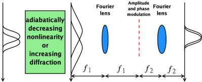
Figure 1: (color online). Schematics of the spatial quantum enhancement setup via adiabatic soliton expansion.

So far we have worked in the paraxial regime, so a 4$f$ imaging system with spatial phase modulation in the Fourier plane can effectively mimic the behavior of negative refraction. Consider the system depicted in Fig. 1. After the beam goes through the nonlinear medium and the first Fourier lens, in the Fourier plane, the multiphoton amplitude becomes

$$\psi(x_{1},...,x_{N}) \propto\phi\left(\frac{2\pi x_{1}}{\lambda f_{1}},...,\frac{2\pi x_{N}}{\lambda f_{1}}\right).$$ (28)

A quadratic spatial phase modulation in the Fourier plane, by a lens for example, can hence act as negative refraction in the paraxial regime and cancel the quantum dispersion term.

In general, Fourier-domain modulation with a transfer function $H(k)$ can be used to shape $G(k)$, if the ultimate multiphoton state is achieved, because all photons have coincident momenta, resulting in an output given by $G(k)H^{N}(k)$. A desired multiphoton interference pattern $|g(NX)|^{2}$ can hence be engineered by spatial modulation in the Fourier plane.

If the ultimate multiphoton state is achieved via adiabatic soliton expansion, the bandwidth of the optical beam is the same as that of $G(k)$, which is on the order of $1/(\sqrt{N}W_{0})$, and is much smaller than the resolution limit. The second Fourier lens in Fig. 1 should therefore have a small focal length $f_{2}$ to demagnify the optical beam and increase the bandwidth of $G(k)$.

Current technology should be able to expand a spatial soliton with $N\sim 10^{10}$ photons by a few times before decoherence effects, such as loss, become significant. However, for quantum lithography, an ideal high-number-photon absorption material is difficult to obtain, so a giant Kerr nonlinearity, such as that theorized in a coherent medium schmidt , is required to produce a few-photon soliton.

In conclusion, spatial quantum enhancement effects are studied under a general framework. It is shown that the multiphoton absorption rate is reduced if the lithographic resolution is enhanced. The use of adiabatic soliton expansion is proposed to beat the spatial standard quantum limits for an arbitrary number of photons.

Discussions with Demetri Psaltis and financial support by the Defense Advanced Research Projects Agency (DARPA) are gratefully acknowledged.

References

- (1) C. A. J. Putman, B. G. De Grooth, N. F. Van Hulst, and J. Greve, J. Appl. Phys. 72, 6 (1992).
- (2) S. Kamimura, Appl. Opt. 26, 3425 (1987).
- (3) C. Fabre, J. B. Fouet, and A. Mâitre, Opt. Lett. 25, 76 (2000); S. M. Barnett, C. Fabre, and A. Mâitre, Eur. Phys. J. D 22, 513 (2003).
- (4) N. Treps, U. Andersen, B. Buchler, P. K. Lam, A. Maître, H.-A. Bachor, and C. Fabre, Phys. Rev. Lett. 88, 203601 (2002).
- (5) M. Born and E. Wolf, Principles of Optics (Cambridge University Press, Cambridge, UK, 1999).
- (6) A. N. Boto, P. Kok, D. S. Abrams, S. L. Braunstein, C. P. Williams, and J. P. Dowling, Phys. Rev. Lett. 85, 2733 (2000); P. Kok, A. N. Boto, D. S. Abrams, C. P. Williams, S. L. Braunstein, and J. P. Dowling, Phys. Rev. A63, 063407 (2001).
- (7) G. Björk, L. L. Sánchez-Soto, and J. Söderholm, Phys. Rev. Lett. 86, 4516 (2001); G. Björk, L. L. Sánchez-Soto, and J. Söderholm, Phys. Rev. A64, 013811 (2001).
- (8) M. D’Angelo, M. V. Chekhova, and Y. Shih, Phys. Rev. Lett. 87, 013602 (2001).
- (9) V. Giovannetti, S. Lloyd, and L. Maccone, Nature (London)412, 417 (2001).
- (10) M. Tsang, e-print quant-ph/0603088 [submitted to Phys. Rev. Lett. ].
- (11) L. Mandel and E. Wolf, Optical Coherence and Quantum Optics (Cambridge University Press, Cambridge, UK, 1995).
- (12) P. L. Hagelstein, Phys. Rev. A54, 2426 (1996).
- (13) J. Javanainen and P. L. Gould, Phys. Rev. A41, 5088 (1990); J. Perina, Jr., B. E. A. Saleh, and M. C. Teich, Phys. Rev. A57, 3972 (1998).
- (14) Y. Lai and H. A. Haus, Phys. Rev. A40, 844 (1989); ibid. 40, 854 (1989).
- (15) V. G. Veselago, Sov. Phys. Usp. 10, 509 (1968); J. B. Pendry, Phys. Rev. Lett. 85, 3966 (2000).
- (16) H. Schmidt and A. Imamoglu, Opt. Lett. 21, 1936 (1996).