Genetic Algorithm Optimization of Entanglement

Abstract

We present an application of a genetic algorithmic computational method to the optimization of the concurrence measure of entanglement for the cases of one dimensional chains, as well as square and triangular lattices in a simple tight-binding approach in which the hopping of electrons is much stronger than the phonon dissipation.

DOI: 10.1103/PhysRevA.74.052308 PACS number(s): 03.67.Hk, 03.65.Ud, 71.10.Fd

I Introduction

Entanglement has been described as an important characteristic for quantum information and quantum computation nc2000 . In the following, the quantity of interest will be the concurrence measure of entanglement introduced by Wootters wootters1 . It will be studied for various kinds of condensed-matter lattice systems and the main focus will be on calculating optimized entangled states using genetic algorithms genschemas1 . To the best of our knowledge, at the present time there exists only a paper by Prashant on the application of genetic algorithms to evolving quantum circuits prashant .

The motivation for our work resides in recent studies about maximum nearest-neighbor entanglement romls31 ; romls32 . In these cases, a $N$-qubit ring in a translationally invariant quantum state has been considered. Under certain conditions, O’Connor and Wooters romls31 have found formulas to obtain the maximum possible nearest-neighbor entanglement. Moreover, they have compared this quantity with the entanglement produced off an antiferromagnetic state of a ring with an even number of spin-$\frac{1}{2}$ particles. Also, there have been studies of concurrence for nearest-neighbors in finite clusters with the purpose to see its behavior in two dimensions. In particular, this was carried on for square, triangular and Kagomé lattices romls33 . Further studies focus on systems with higher order entanglement, that is, when subsystem $A$ is bigger than two qubits br01 .

In the lattice systems of this research, qubits are represented by sites in a lattice or a chain. The two computational basis $|0\rangle$ and $|1\rangle$ are represented by occupied and empty sites, respectively. Using this representation, the concurrence can be calculated for different fillings. This approach might be useful for physical experiments involving electron control (e.g., quantum dots recipes-spinbased ).

The electronic system will be described by a tight-binding Hamiltonian of the form

$$\hat{H}=\sum_{i}\varepsilon_{i}\hat{n}_{i}+\sum_{\langle ij\rangle}t_{ij}\hat{c}_{i}^{\dagger}\hat{c}_{j}~{},$$ (1)

where, for simplicity, we will consider spinless electrons. In (1) $\hat{c}_{i}^{\dagger}$ ($\hat{c}_{j}$) is the usual creation (annihilation) operator of a spinless electron at site $i$, whereas $\hat{n}_{i}=\hat{c}_{i}^{\dagger}\hat{c}_{i}$ is the number operator, and $t_{ij}$ is the hopping integral between nearest-neighbors (NN) and next-nearest-neighbors (NNN) sites $i$ and $j$. $\varepsilon_{i}$ is the on-site energy for atom $i$. For simplicity, we work with the same kind of atoms and we take $\varepsilon_{i}=0$. There exist physical systems which can be modeled using a similar approach as here, most notably the polyacetylene systems Su80 in the static approximation (without phonons).

Notice that we are using a one-body Hamiltonian. For this case the ground state wave function can be obtained simply by filling the lowest one-body eigenstates. The corresponding eigenvalues are obtained by diagonalizing the matrix Hamiltonian as expressed in the one-body basis. In this case, one can always find a linear transformation of $c_{i}^{\dagger}$ ($c_{i}$) leading to a diagonal form of the Hamiltonian.

Specifically, our tight-binding Hamiltonian $\hat{H}=-\sum_{ij}t_{ij}\hat{c}_{i}^{\dagger}\hat{c}_{j}$ can be written as $\hat{H}=\sum_{k}\varepsilon_{k}\hat{c}_{k}^{\dagger}\hat{c}_{k}$, where $c_{i}^{\dagger}=\sum_{k}\alpha_{ik}\hat{c}_{k}^{\dagger}$ and $c_{i}=\sum_{k}\alpha_{ik}^{*}\hat{c}_{k}$. For periodic systems with only NN hopping integrals ($t_{ij}=t$) Zan , the Hamiltonian $\hat{H}$ can be diagonalized through the Fourier transformations $\hat{c}_{l}=\frac{1}{\sqrt{N}}\sum_{k=1}^{N}\exp(i2\pi lk/N)\hat{c}_{k}$ and the complex-conjugated counterpart, therefore $\hat{H}$ takes the form

$$\hat{H}=-2t\sum_{k=1}^{N}\cos(2\pi k/N)\hat{c}_{k}^{\dagger}\hat{c}_{k}~{}.$$ (2)

On the other hand, for a nonperiodic system with arbitrary hopping integrals it is not possible to get an analytic diagonalization procedure. For the simplest nonanalytic case of a system of $N$ atomic sites and nearest-neighbor hopping integrals, one should diagonalize a Hamiltonian matrix of tridiagonal form:

$$\hat{H}=\left(\begin{array}[]{ccccccc}0&-t_{12}&0&0&\cdots&\cdots&0\\ -t_{12}&0&-t_{23}&0&\cdots&\cdots&0\\ 0&-t_{23}&0&-t_{34}&\cdots&\cdots&0\\ 0&0&-t_{34}&0&-t_{45}&\cdots&0\\ \cdots&\cdots&\cdots&\cdots&\cdots&\cdots&\cdots\\ 0&0&\cdots&\cdots&\cdots&0&-t_{(N-1)N}\\ 0&0&\cdots&\cdots&0&-t_{(N-1)N}&0\end{array}\right)~{}.$$ (3)

We have used the LAPack subroutines lapack to diagonalize this type of Hamiltonian matrices through the QR algorithm as well as more complicated forms resulting from next-nearest interactions, where the Householder reduction to tridiagonal forms is applied first. The eigenvectors for $K$ fermions can be obtained in a direct way using the preceding equations and are given by the tensorial product of the one-body eigenvectors,

$$|{\bf k}_{K}\rangle=\hat{c}_{k_{1}}^{\dagger}\hat{c}_{k_{2}}^{\dagger}\cdots\hat{c}_{k_{K}}^{\dagger}|0\rangle~{}.$$ (4)

Thus, it is clear that for the ground state we require the lowest levels to be occupied.

Moreover, through a Jordan-Wigner transformation the spinless fermion Hamiltonian can be rewritten as a $XX$ spin-$\frac{1}{2}$ chain. In the spinless fermion case, each lattice site is either occupied or free, whereas in the spin polarization case each lattice site can have the spin up or down. It is well known that oxides and fluorides of transition metals, e.g., MnO, NiO and MnF₂, FeF₂, CoF₂, respectively, are described by such simple spin Hamiltonians gpp03 .

Wootters’ formula that we used to calculate the concurrence is obtained in the Appendix and is given by

$$C=\max\{0,2|\rho_{23}|-2\sqrt{\rho_{11}\rho_{44}}\}=2\,\max\{0,|\rho_{23}|-\sqrt{\rho_{11}\rho_{44}}\}~{}.$$ (5)

The concurrence calculations in Sec. II are always a sum over all the pairs of sites divided to the total number of sites. Section III contains some conclusions and the Appendix is devoted to the mathematics of the concurrence formula.

II Optimizing Entanglement using Genetic Algorithms

We pass now to the main goal of the paper which is the maximization of entanglement using genetic algorithms. Specifically, we will consider the ground state of a spinless system modeled by the tight binding Hamiltonian given in Eq. (1).

We recall that genetic algorithms (GAs) were invented by John Henry Holland in the 1960s and were developed by him and his students and colleagues at the University of Michigan in the 1960s and the 1970s. Holland’s goal was not to design algorithms to solve specific problems, but rather to formally study the phenomenon of adaptation as it occurs in nature and to develop ways in which the mechanisms of natural adaptation might be imported into computer systems.

Much alike nature, Holland’s GA is a method for moving from one population of “chromosomes” (e.g., strings of characters or numbers) to a new population by using a kind of “natural selection” together with the genetics-inspired operators of crossover, mutation, and inversion (this last operator is rarely used nowadays).

The genetic pseudoalgorithm employed by us here goes as follows:

1. Read input parameters including type of lattice, sites in the system, number of generations, crossover probability, mutation probability, etc.

2. Build a table with indices of the nearest neighbors of each site. A table including also next-nearest neighbors can be built as well.

3. Using the neighbor table, identify the specific places in the Hamiltonian matrix where “bonds” occur. Each place represents a valid $t_{ij}$ entries and will be stored in a special array. This array will be considered hereafter as a chromosome.

4. Allocate two arrays, “generation0” and “generation1” composed of chromosomes.

5. Construct an additional chromosome called “best” with initial random numbers between $(0,5)$.

6. For a given range of filling repeat:

   • Initialize “generation0” with random values in the range $(0,5)$.

   • Make the first chromosome of “generation0” equal to “best”.

   • For a given number of generations repeat:

     • Decode each chromosome in “generation0” into a Hamiltonian matrix, diagonalize it and calculate the total concurrence between all nearest neighbors of the system. In other words, calculate fitness for each individual in “generation0”.

     • Make “best” equal to the chromosome with highest value of fitness in “generation0”

     • Print the value of the average fitness of the population of “generation0” and fitness of “best” in output files.

     • Apply the selection operator: Use crossover and mutation operators on chromosomes in “generation0” to create new chromosomes into “generation1”.

     • Make “generation0” equal to “generation1”.

     • Make the first chromosome in “generation0” equal to “best”.

   • Find the chromosome with the maximum fitness. Print its fitness value in an output file.

To make the calculations tractable the biggest system that we considered was of 49 sites with 800 generations for which the optimization procedure has taken about three days. In all calculations we have worked with the probability of crossover $p_{c}=0.70$ and the probability of mutation $p_{m}=0.002$.

II.1 One-dimensional chains

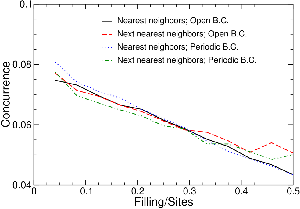
Figure 1: (Color online) Optimized concurrence as a function of band filling for a linear chain with 24 sites. $250$ generations; population $=400$. Note that in all figures the quantities plotted are dimensionless and the values of the parameters $p_{c}$ and $p_{m}$ are fixed at $0.70$ and $0.002$, respectively.

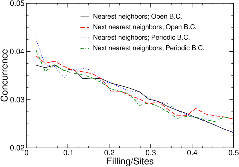
Figure 2: (Color online) Optimized concurrence as a function of band filling for a linear chain with 44 sites. $250$ generations; population $=400$.

We begin the analysis of entanglement maximization using genetic algorithms with the simplest case of small lineal chains with and without periodic boundary conditions. In Figs. 1 and 2 we present results of concurrence as a function of percentage filling for two chains with $24$ and $44$ sites, respectively. Besides nearest-neighbor interactions, we have also considered interactions with both nearest neighbors and next-nearest neighbors in the Hamiltonian. The population size remained at $400$ individuals and the generations were kept at $250$. Later on, the role of the number of generations will become apparent.

From the figures, it can be noticed that in the case of nearest-neighbor interactions with and without periodic boundary conditions, concurrence as function of filling is smoother than in the cases where next nearest neighbors are also considered. This can be due to a larger size in the chromosomes in the latter case and a greater number of generations are necessary to obtain a similar behavior than its only-nearest-neighbors counterpart. We can only conclude that a greater number of generations and possibly a greater size in the population is necessary to overcome these oscillations.

Also, notice that cases including next nearest neighbors cannot yield lower results than the only nearest neighbors case. This is because the chromosomes from the former case contain the chromosomes of the latter (i.e., the NN case is a subset of the NNN case), which offers the possibility to explore a wider spectrum of solutions. In the case where this extra space yielded only lower results, the best chromosomes would be those of the NN space. This phenomenon can be most clearly noticed near half filling. Once again, this behavior is a consequence of a greater number of generations.

At this point, it is important to remember that there are various parameters responsible for a larger chromosome in this kind of system. These parameters are the size of the system, the periodic boundary conditions and bringing next-nearest-neighbors interactions into play. A larger chromosome would allow an exploration of a wider solution space but on the other hand it is expected to decrease the convergence time.

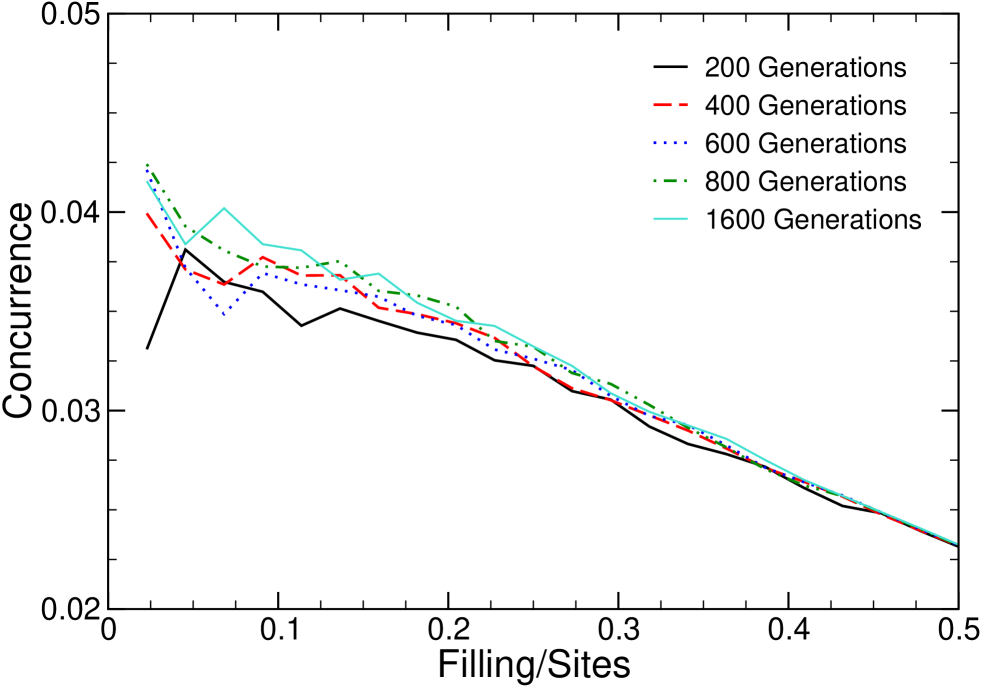
Figure 4: (Color online) Optimized concurrence for different number of generations in a one-dimensional 44-site lattice using periodic boundary conditions, population size $=400$.

We have already mentioned the possibility of a greater number of generations affecting directly the smoothness of the concurrence. We addressed this question by running two cases depicted in Figs. 3 and 4, where the former does not consider periodic boundary conditions while the latter does.

In both cases we have set a $44$-site chain with a population size of $400$. Only the interactions between nearest neighbors were taken into account.

Both figures confirm our early supposition about increasing the number of generations since the correlation functions look increasingly smoother. Notice, however, that certain roughness still remains. Some possible solutions consist of increasing the size of the population, dynamically change the mutation probability (when variation between individuals begins to narrow) and raising the number of generations further more. Different selection methods could also be considered because an inefficient parent selection could lead to slow evolution of the system. Even though it is clear that individuals with better fitness are obtained, notice how in Fig. 3 the best chromosome near $0.05$ filling was obtained with $600$ generations despite having cases with up to three times more generations.

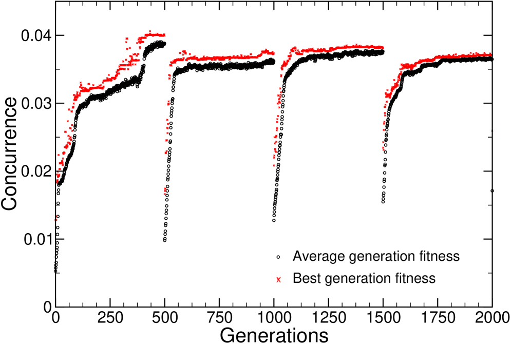
Figure 6: (Color online) Detail of Fig. 5 for the first $2000$ generations.

In Fig. 5 (for its more detailed structure up to $2000$ generations see Fig. 6) we follow the evolution (optimization) of concurrence for each filling in a $44$-site chain with periodic boundary conditions and interactions only between nearest neighbors. The population size for this calculation was $350$ and the number of generations was $500$ per filling. The average fitness per population is compared with the fitness from the best chromosome in the population. Notice how the population always follows closely the evolution of the best chromosome. Transitions between different fillings are readily noticed through a drop in average fitness. A very remarkable feature is that the best chromosome for a certain filling ranks high for the next filling but is not the highest. In other words, there are different best chromosomes for different band fillings. We also notice that the bottom dots correspond to the average concurrence for randomly disordered populations and that the average concurrences for the subsequent optimized GA populations are always better than the disordered cases.

Another remarkable characteristic about Fig. 5 is its symmetry around half-band filling. This property is due to the fact that this is a bipartite lattice and consequently its physical properties are symmetric because of an electron-hole transformation. The fact that the results presented show this property reassures the validity of our calculations.

II.2 Two-dimensional systems

We will study now the optimization of concurrence in two-dimensional systems modeled by means of the same tight-binding Hamiltonian.

II.2.1 Square lattices

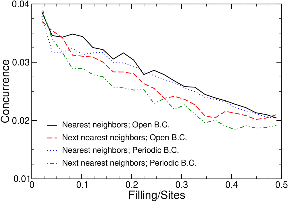
Figure 7: (Color online) Optimized concurrence for a square lattice comparing nearest-neighbor interactions, next-nearest-neighbor interactions and boundary conditions. $600$ generations; population size $=350$.

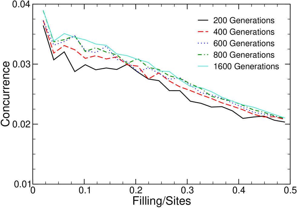
Figure 8: (Color online) Optimized concurrence for a square lattice comparing number of generations for nearest-neighbor interactions, periodic boundary conditions, population size $=400$.

In Figs. 7 and 8 we display the concurrence as a function of band filling for a 7$\times$7 square lattice.

Figure 7 presents a comparison between systems using nearest-neighbor and next-nearest-neighbor interactions as well as periodic and open boundary conditions. The number of generations for these cases has been chosen $600$ and the population size $350$. It is worth mentioning that in general the cases with interactions only between nearest-neighbors rank slightly higher in its concurrence value. This is a somewhat unexpected result that may be attributed to various factors including selection methods and number of generations. Possible reasons for this behavior were addressed in the preceding section.

To study the effect of the number of generations on the optimized value of concurrence and the smoothness of the curve, we present calculations for four different cases in Fig. 8. In these cases, population size was kept at $400$. It is clear that by raising this number we are able to obtain better optimized solutions and the concurrence curve tends to be smoother.

II.2.2 Triangular lattices

Finally, we have made calculations for not bipartite lattices in order to study the effect of frustration on concurrence. It has already been mentioned that these kinds of lattices are not symmetric under an electron-hole transformation. This is the reason why their physical properties differ completely between lower and upper sections of band filling.

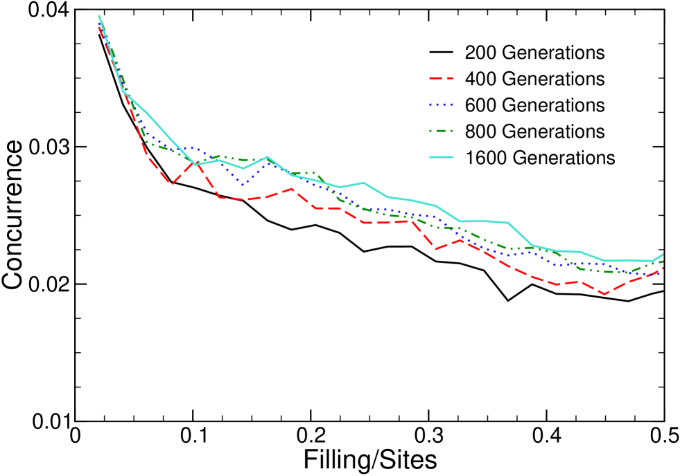
Figure 10: (Color online) Optimized concurrence for a triangular lattice comparing number of generations for nearest-neighbor interactions, periodic boundary conditions, population size $=400$.

As a particular case of a nonbipartite lattice, we have considered a triangular lattice with $49$ sites. Results of our calculations are shown in Figs. 9 and 10.

In Fig. 9 a population size of $350$ has been used and the system has been allowed to go up to $600$ generations. As in the preceding sections, this case includes the interaction between nearest and next-nearest neighbors, as well as open and periodic boundary conditions. Once again, we find better optimizations for nearest-neighbor interactions. It is important to remember that we are dealing with a more complex chromosome, as sites in this kind of lattice have a greater number of neighbors than one dimensional systems. This is also a cause for a lower time in convergence as the solution space increases considerably.

The effect of the number of generations can be examined in Fig. 10. These results demonstrate the slow convergence when calculating this kind of system. Notice that, although oscillations decrease and better individuals are found, efficiency narrows between the cases with $600$ and $800$ generations.

III Conclusions

We have implemented computational techniques –more specifically genetic algorithms– to optimize entanglement in systems modeled according to a tight-binding Hamiltonian. The qubits in all these studies have been described as sites in the system and the computational basis as occupied or empty sites.

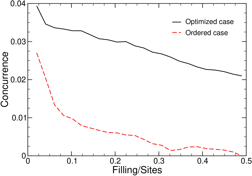
Figure 11: (Color online) Concurrence for the optimized and ordered cases in a $49$ sites square lattice using nearest-neighbor interactions and periodic boundary conditions $800$ generations; population size $=400$.

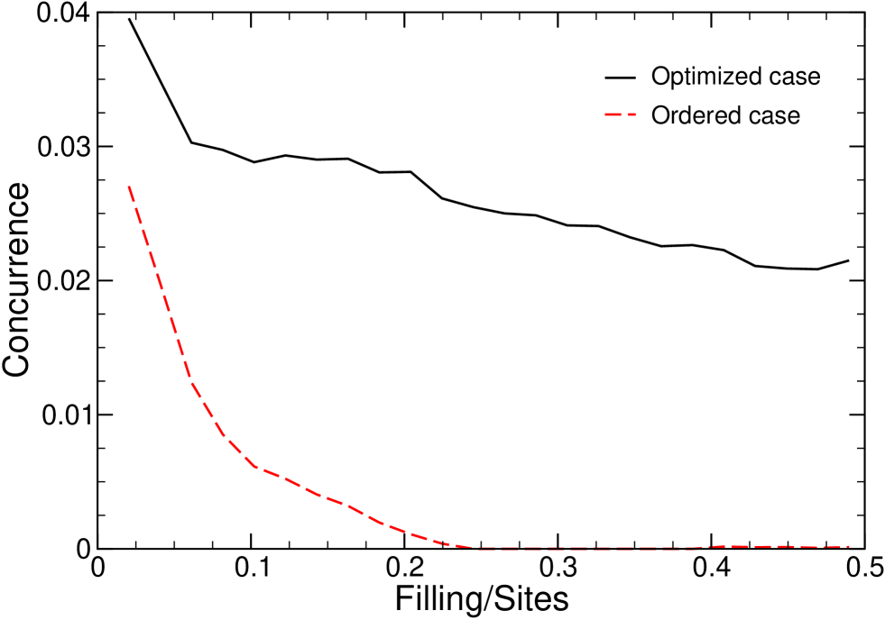
Figure 12: (Color online) Concurrence for the optimized and ordered cases in a $49$ sites triangular lattice under the same conditions as in the previous figure.

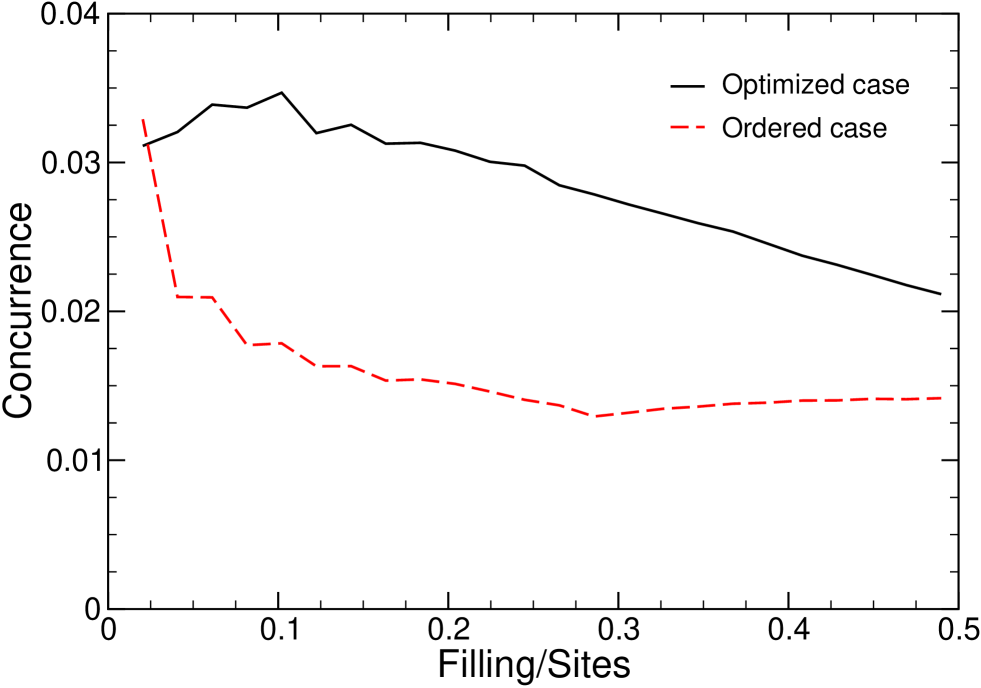
Figure 13: (Color online) Comparison between the optimized and the ordered case in a one-dimensional system of $49$ sites. The calculation parameters were identical to those of Figs. 11 and 12.

Our application of genetic algorithms has proven to be valuable, since we obtained configurations which yield better results for concurrence in the randomly disordered one-dimensional case as discussed in Sec. II A (in fact, we have partial results confirming this statement for two-dimensional cases as well). Moreover, the GA optimization provided better results even with respect to the ordered cases as can be noticed in Figs. 11, 12, and 13.

We finally mention that the optimal Hamiltonian for the one-dimensional case with periodic boundary conditions corresponds to dimerized chain for which the coupling coefficients take alternate high-low values in the half filling region. This structural phase transition has been found in the polyacetylene chains and suggests that optimal entanglement can be obtained in the dimerized phase of the polyacetylene. We have also some evidence of this behavior in two-dimensional systems. These results will be reported elsewhere.

Quantum computation and quantum information are still a long way to go. Nevertheless, these areas seems to be a logical and necessary step in tomorrow’s technological world. In this scenario, quantum entanglement will play a critical role, and our work attempts to be another step towards better understanding it.

APPENDIX: THE CONCURRENCE

To calculate the concurrence we need first the density matrix $\rho_{A}$ for qubits $i,j$, which is the trace over system $B$ of all the possible states $|\psi_{AB}\rangle\langle\psi_{AB}|$. The general state function for this system is

$$|\psi_{AB}\rangle=\sum_{n}\alpha_{n}|\psi_{A}\rangle|\psi_{B}\rangle$$ (6)

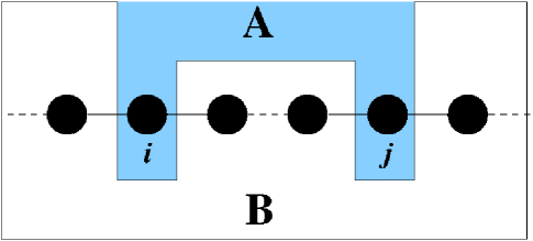
Figure 14: (Color online) Schematic illustration of the partition of the system of interest into two subsystems for the calculation of the concurrence between sites $i$ and $j$.

where, for a system of $N$ sites, $n$ goes through all the $2^{N}$ possible combinations in the computational basis (e.g., $|00\ldots 00\rangle\rightarrow|11\ldots 11\rangle$). Subsystem $A$ is comprised of the two qubits of interest in the sites $i,j$ (i.e., $|\psi_{i}\rangle\otimes|\psi_{j}\rangle$, see also Fig. 14). For a specific system of $N$ sites, there are $N_{1}$ occupied and $N-N_{1}$ not occupied sites. Our two-qubit subsystem $A$ has, naturally, four possible states –namely $|00\rangle,|01\rangle,|10\rangle$, and $|11\rangle$– therefore Eq. (6) can be decomposed in the following manner:

$$|\psi_{AB}\rangle=\sum_{m}a_{m}|00\rangle\otimes|\psi_{B}^{m}\rangle+\sum_{o}b_{o}|01\rangle\otimes|\psi_{B}^{o}\rangle+\sum_{p}c_{p}|10\rangle\otimes|\psi_{B}^{p}\rangle+\sum_{q}d_{q}|11\rangle\otimes|\psi_{B}^{q}\rangle.$$ (7)

In this equation, the sums run for all the possible combinations in the $|\psi_{B}\rangle$ space such that the number $N_{1}$ of occupied sites is preserved. For example, if $|\psi_{A}\rangle=|01\rangle$, system $B$ is left with $N_{1}-1$ occupied sites.

To obtain the reduced density matrix it is necessary to perform the trace over system $B$,

$$\rho_{A}=\sum_{l=1}^{2^{N-2}}\big{(}\langle I|\otimes\langle\psi_{B}^{l}|\big{)}|\psi_{AB}\rangle\langle\psi_{AB}|\big{(}|I\rangle\otimes|\psi_{B}^{l}\rangle\big{)}.$$ (8)

It is clear that applying this operation will not eliminate those terms whose elements in the $B$ subsystem in $|\psi_{AB}\rangle\langle\psi_{AB}|$ have the same number of occupied sites. The terms in system $A$ that are left after the trace operation are of the kind $|00\rangle\langle 00|$, $|01\rangle\langle 01|$, $|01\rangle\langle 10|$, $|10\rangle\langle 01|$, $|10\rangle\langle 10|$, and $|11\rangle\langle 11|$.

The $|00\rangle\langle 00|$ element is spared after the trace operator because its $|\psi_{B}^{m}\rangle$ elements contain the same quantity of occupied sites (i.e., $N_{1}$ sites). This is a similar case with the $|11\rangle\langle 11|$ elements where the $|\psi_{B}^{q}\rangle$ wave functions contain $N_{1}-2$ occupied sites.

In the case of $|01\rangle\langle 01|$, $|01\rangle\langle 10|$, $|10\rangle\langle 01|$, and $|10\rangle\langle 10|$ elements, notice how their $|\psi_{B}^{o,p}\rangle$ wave functions have the same number of occupied sites ($N_{1}-1$).

Finally, the elements in the reduced density matrix are

$$\rho_{A}=\left(\begin{array}[]{cccc}\rho_{11}&0&0&0\\ 0&\rho_{22}&\rho_{23}&0\\ 0&\rho_{32}&\rho_{33}&0\\ 0&0&0&\rho_{44}\end{array}\right)~{}.$$ (9)

For $\rho_{A}$ to be a valid density matrix, it must be Hermitic ($\rho_{A}=\rho_{A}^{\dagger*}$) and its trace be equal to $1$. This means that $\rho_{32}=\rho_{23}^{*}$ and $\rho_{11}+\rho_{22}+\rho_{33}+\rho_{44}=1$ so it is necessary to calculate only four elements of the matrix.

In order to calculate each of these reduced density matrix elements, the second quantization approach will be used.

The first element of the matrix, $\rho_{11}$ can be realized as follows

$$\rho_{11}=\langle\psi_{AB}|\big{(}1-\hat{n}_{i}\big{)}\big{(}1-\hat{n}_{j}\big{)}|\psi_{AB}\rangle~{},$$ (10)

where the operator $\hat{n}_{j}$ projects on all the elements of the type $|x1\rangle\otimes|\psi_{B}\rangle$ and after applying $(1-\hat{n}_{j})$ we end up with all the elements that do not occupy the site $j$ (i.e., $|x0\rangle\otimes|\psi_{B}\rangle$). A similar approach follows $(1-\hat{n}_{i})$ and after applying the bra operation we are left only with the coefficients of all the $|00\rangle\otimes|\psi_{B}\rangle$ states.

The other elements are obtained likewise with the following operators: $\rho_{22}=\langle\psi_{AB}|\big{(}1-\hat{n}_{i}\big{)}\hat{n}_{j}|\psi_{AB}\rangle$, $\rho_{33}=\langle\psi_{AB}|\hat{n}_{i}\big{(}1-\hat{n}_{j}\big{)}|\psi_{AB}\rangle$, $\rho_{44}=\langle\psi_{AB}|\hat{n}_{i}\hat{n}_{j}|\psi_{AB}\rangle$, and $\rho_{23}=\langle\psi_{AB}|c_{j}c_{i}^{\dagger}|\psi_{AB}\rangle$.

In the matrix element $\rho_{23}$, $c_{i}^{\dagger}$ maintains only those states of the form $|0x\rangle\otimes|\psi_{B}\rangle$ transforming them into $|1x\rangle\otimes|\psi_{B}\rangle$. Out of this set of states, $c_{j}$ deletes all states of the type $|x0\rangle\otimes|\psi_{B}\rangle$ and we end up with states $|10\rangle\otimes|\psi_{B}\rangle$.

It is very easy to show that the $\rho_{A}$ elements can be calculated as average quantities of the complete ground-state wave function. For example,

$$\rho_{11}=\langle\psi_{AB}|\psi_{AB}\rangle-\langle\psi_{AB}|\hat{n}_{i}|\psi_{AB}\rangle-\langle\psi_{AB}|\hat{n}_{j}|\psi_{AB}\rangle+\langle\psi_{AB}|\hat{n}_{i}\hat{n}_{j}|\psi_{AB}\rangle\\ =1-\langle\hat{n}_{i}\rangle-\langle\hat{n}_{j}\rangle+\langle\hat{n}_{i}\hat{n}_{j}\rangle.$$ (11)

The other elements are obtained similarly, $\rho_{22}=\langle\hat{n}_{j}\rangle-\langle\hat{n}_{i}\hat{n}_{j}\rangle$, $\rho_{33}=\langle\hat{n}_{i}\rangle-\langle\hat{n}_{i}\hat{n}_{j}\rangle$, $\rho_{44}=\langle\hat{n}_{i}\hat{n}_{j}\rangle$, $\rho_{23}=\langle c_{j}c_{i}^{\dagger}\rangle$.

Concurrence is an entanglement monotone in its own right (i.e., positive or zero for any density matrix $\rho$; $0$ for factorizable states and $1$ for the Bell states). A simple formula for the concurrence has been worked out by Wootters in 1998 wootters1 ,

$$C(\rho)=\textrm{max}\{0,\lambda_{1}-\lambda_{2}-\lambda_{3}-\lambda_{4}\},$$ (12)

where the $\lambda$ coefficients are the square roots of the eigenvalues of the non-Hermitian matrix $\rho_{A}\tilde{\rho_{A}}$ in decreasing order. The formula applies for the density matrix of the subsystem with the pair of qubits [$\rho_{A}=$tr_B($\rho$)]. The density matrix $\tilde{\rho}$ is defined through a spin flip transformation expressed in terms of the imaginary Pauli matrix $\sigma_{y}$ as follows

$$\tilde{\rho_{A}}=\big{(}\sigma_{y}\otimes\sigma_{y}\big{)}\rho_{A}^{*}\big{(}\sigma_{y}\otimes\sigma_{y}\big{)}.$$ (13)

This leads to

$$\tilde{\rho_{a}}=\left(\begin{array}[]{cccc}0&0&0&-1\\ 0&0&1&0\\ 0&1&0&0\\ -1&0&0&0\end{array}\right)\left(\begin{array}[]{cccc}\rho_{11}^{*}&0&0&0\\ 0&\rho_{22}^{*}&\rho_{23}^{*}&0\\ 0&\rho_{32}^{*}&\rho_{33}^{*}&0\\ 0&0&0&\rho_{44}^{*}\end{array}\right)\left(\begin{array}[]{cccc}0&0&0&-1\\ 0&0&1&0\\ 0&1&0&0\\ -1&0&0&0\end{array}\right)\\ =\left(\begin{array}[]{cccc}\rho_{44}^{*}&0&0&0\\ 0&\rho_{33}^{*}&\rho_{32}^{*}&0\\ 0&\rho_{23}^{*}&\rho_{22}^{*}&0\\ 0&0&0&\rho_{11}^{*}\end{array}\right)~{}.$$ (14)

Now we are able to construct the non-Hermitian matrix $\rho_{A}\tilde{\rho_{A}}$

$$\rho_{A}\tilde{\rho_{A}}=\left(\begin{array}[]{cccc}\rho_{11}\rho_{44}^{*}&0&0&0\\ 0&\rho_{22}\rho_{33}^{*}+\rho_{23}\rho_{23}^{*}&\rho_{22}\rho_{32}^{*}+\rho_{23}\rho_{22}^{*}&0\\ 0&\rho_{32}\rho_{33}^{*}+\rho_{33}\rho_{23}^{*}&\rho_{32}\rho_{32}^{*}+\rho_{33}\rho_{22}^{*}&0\\ 0&0&0&\rho_{11}^{*}\rho_{44}\end{array}\right)~{}.$$ (15)

However, $\rho_{A}$ is indeed Hermitian so the following relationships are taken into account: $\rho_{11}=\rho_{11}^{*}$, $\rho_{22}=\rho_{22}^{*}$, $\rho_{32}=\rho_{23}^{*}$, $\rho_{33}=\rho_{33}^{*}$, and $\rho_{44}=\rho_{44}^{*}$. Therefore, the matrix $\rho_{A}\tilde{\rho_{A}}$ has the form

$$\rho_{A}\tilde{\rho_{A}}=\left(\begin{array}[]{cccc}\rho_{11}\rho_{44}&0&0&0\\ 0&\rho_{22}\rho_{33}+|\rho_{23}|^{2}&2\rho_{22}\rho_{23}&0\\ 0&2\rho_{33}\rho_{23}^{*}&\rho_{22}\rho_{33}+|\rho_{23}|^{2}&0\\ 0&0&0&\rho_{11}\rho_{44}\end{array}\right).$$ (16)

In a block diagonal matrix, the eigenvalues are simply the eigenvalues of individual blocks, so two eigenvalues are readily available. The other two are obtained from the following determinant

$$\left(\begin{array}[]{cc}\rho_{22}\rho_{33}+|\rho_{23}|^{2}-\lambda&2\rho_{22}\rho_{23}\\ 2\rho_{33}\rho_{23}^{*}&\rho_{22}\rho_{33}+|\rho_{23}|^{2}-\lambda\\ \end{array}\right).$$ (17)

This gives

$$\lambda=\rho_{22}\rho_{33}+|\rho_{23}|^{2}\mp 2\sqrt{\rho_{22}\rho_{33}}|\rho_{23}|~{}.$$ (18)

Thus, the four possible values of the $\lambda$ coefficients are as follows:

$$\lambda_{a}=(\sqrt{\rho_{22}\rho_{33}}-|\rho_{23}|)^{2},\quad\lambda_{b}=(\sqrt{\rho_{22}\rho_{33}}+|\rho_{23}|)^{2},\quad\lambda_{c}=\rho_{11}\rho_{44},\quad\lambda_{d}=\rho_{11}\rho_{44}.$$ (19)

Finally, the square roots of these lambda coefficients are directly employed in (12).

Noticing that $\lambda_{b}$ is the largest eigenvalue, the latter results leads immediately to Wootters’ formula Eq. (2).

Figure 3: (Color online) Optimized concurrence for different number of generations in a one-dimensional 44-site lattice. Open boundary conditions, population size $=400$.

Figure 5: (Color online) Best and average fitness for each generation in a one-dimensional 44-site lattice subjected to periodic boundary conditions, nearest-neighbor interactions, for $500$ generations, population size of $350$.

Figure 9: (Color online) Optimized concurrence for a triangular lattice comparing nearest-neighbor interactions, next nearest neighbor interactions and boundary conditions. $600$ generations; population size $=350$.

References

- (1) M. Nielsen and I. Chuang, Quantum Computation and Quantum Information, (Cambridge University Press, Cambridge, 2000).
- (2) W.K. Wooters, Phys. Rev. Lett. 80, 2245 (1998).
- (3) M.Mitchell, An Introduction to Genetic Algorithms, (A Bradford Book, The MIT Press, Cambridge, MA, 1999).
- (4) Prashant, “Evolving quantum circuits using genetic algorithm”, quant-ph/0511036.
- (5) K. M. O’Connor and W. K. Wootters, Phys. Rev. A 63, 052302 (2001).
- (6) W. K. Wootters, Contemp. Math. 305, 299 (2002).
- (7) V. Subrahmanyam, Phys. Rev. A 69, 022311 (2004).
- (8) H.J. Briegel and R. Raussendorf, Phys. Rev. Lett. 86, 910 (2001).
- (9) V. Cerletti, W. A. Coish, O. Gywat, and D. Loss, Nanotechnology 16, R27 (2005).
- (10) W. P. Su, J. R. Schrieffer, and A. J. Heeger, Phys. Rev. B 22, 2099 (1980).
- (11) P. Zanardi and X. Wang, J. Phys. A 35, 7947 (2002).
- (12) Lapack, http://www.netlib.org/lapack
- (13) G. Grosso and G. Pastori Parravicini, Solid State Physics (Academic, San Diego, 2003), p. 631.