Application of the Asymptotic Iteration Method to a Perturbed Coulomb Model

Abstract

We show that the asymptotic iteration method converges and yields accurate energies for a perturbed Coulomb model. We also discuss alternative perturbation approaches to that model.

1 Introduction

The asymptotic iteration method (AIM) is an iterative algorithm for the solution of Sturm–Liouville equations [1, 2]. Although this method does not seem to be better than other existing approaches, it has been applied to quantum–mechanical [4, 5, 3] as well as mathematical problems [6]. For example, the AIM has proved suitable for obtaining both accurate approximate and exact eigenvalues [1, 2, 4, 6, 5, 3] and it has also been applied to the calculation of Rayleigh–Schrödinger perturbation coefficients [5, 7].

Recently, Barakat applied the AIM to a Coulomb potential with a radial polynomial perturbation [5]. By means of a well–known transformation he converted the perturbed Coulomb problem into an anharmonic oscillator. Since straightforward application of the AIM exhibited considerable oscillations and did not appear to converge Barakat resorted to perturbation theory in order to obtain acceptable results [5].

It is most surprising that the straightforward application of the AIM failed for the anharmonic oscillator studied by Barakat [5] since it had been found earlier that the approach should be accurate in such cases [2].

The main purpose of this paper is to verify whether the AIM gives accurate eigenvalues of the perturbed Coulomb model or if its sequences are oscillatory divergent as mentioned above. We also discuss the application of perturbation theory to that model.

In Sec. 2 we present the model and discuss useful scaling relations for the potential parameters. In Sec. 3 we apply the AIM to the perturbed Coulomb model directly; that is to say we do not convert it into an anharmonic oscillator. In Sec. 4 we outline alternative perturbation approaches, and in Sec. 5 we interpret our results and draw conclusions.

2 The model

The problem studied by Barakat [5] is given by the following radial Schrödinger equation

$$\hat{H}\Psi = E\Psi,$$

$$\hat{H} = -\frac{1}{2}\frac{d^{2}}{dr^{2}}+\frac{l(l+1)}{2r^{2}}+V(r)$$

$$V(r) = -\frac{Z}{r}+gr+\lambda r^{2},$$ (1)

where $l=0,1,2,\ldots$ is the angular–momentum quantum number, and the boundary conditions are $\Psi(0)=\Psi(\infty)=0$. We restrict to the case $\lambda>0$ in order to have only bound states; on the other hand, $Z$ and $g$ can take any finite real value.

It is most useful to take into account the scaling relations

$$E(Z,g,\lambda) = Z^{2}E(1,gZ^{-3},\lambda Z^{-4})=|g|^{2/3}E(Z|g|^{-1/3},g|g|^{-1},\lambda|g|^{-4/3})$$ (2)

$$= \lambda^{1/2}E(Z\lambda^{-1/4},g\lambda^{-3/4},1).$$

Notice that we can set either $Z$ or $\lambda$ equal to unity without loss of generality, and that, for example, $E(1,-g,\lambda)=E(-1,g,\lambda)$. Following Barakat [5] we choose $n=0,1,\ldots$ to be the radial quantum number, and we may define a “principal ” quantum number $\nu=n+l+1=1,2,\ldots$.

3 Direct application of the AIM

Barakat mentions that straightforward application of the AIM does not give reasonable results because the sequences oscillate when the number of iteration is greater than $30$ approximately [5]. This conclusion is surprising because it has been shown that the AIM yields accurate results for anharmonic oscillators [2], and Barakat converted the perturbed Coulomb model into one of them[5]. In this section we apply the AIM directly to the original radial Schrödinger equation (1).

By means of the transformation $\psi(r)=\phi(r)y(r)$ we convert the perturbed Coulomb model (1) into a Sturm–Liouville equation for $y(r)$:

$$y^{\prime\prime}(r) = Q(r)y^{\prime}(r)+R(r)y(r)$$

$$Q(r) = -\frac{2\phi^{\prime}(r)}{\phi(r)}$$

$$R(r) = \left\{2[V(r)-E]-\frac{\phi^{\prime\prime}(r)}{\phi(r)}\right\},$$ (3)

where $\phi(r)$ is arbitrary. It seems reasonable to choose

$$\phi(r)=r^{l+1}e^{-\beta r-\alpha r^{2}}$$ (4)

that resembles the asymptotic behaviour of the eigenfunction for a harmonic oscillator when $\beta=0$ or for a Coulomb interaction when $\alpha=0$. It leads to

$$Q(r) = 4\alpha r-\frac{2(l+1)}{r}+2\beta$$

$$R(r) = \left(2\lambda-4\alpha^{2}\right)r^{2}+(2g-4\alpha\beta)r+\frac{2\beta(l+1)-2Z}{r}$$ (5)

$$+2\alpha(2l+3)-2E-\beta^{2}.$$

We can set the values of the two free parameters $\alpha$ and $\beta$ to obtain the greatest rate of convergence of the AIM sequences. From now on we call asymptotic values of $\alpha$ and $\beta$ to such values of those parameters that remove the terms of $R(r)$ that dominate at large $r$; that is to say: $\beta=g/(2\alpha)$ and $\alpha=\sqrt{\lambda/2}$. Since the asymptotic values of the free parameters do not necessarily lead to the greatest convergence rate[2], in what follows we will also look for optimal values of $\alpha$.

The Sturm–Liouville equation (3) with the functions $Q(r)$ and $R(r)$ (5) is suitable for the application of the AIM. We do not show the AIM equations here because they have been developed and discussed elsewhere[1, 2]. Since the AIM quantization condition depends not only on the energy but also on the variable $r$ for non–exactly solvable problems, we have to choose a convenient value for the latter[1, 2]. Later on we will discuss the effect of the value of $r$ on the convergence of the method; for the time being we follow Barakat [5] and select the positive root of $\phi^{\prime}(r)=0$:

$$r_{0}=\frac{\sqrt{8\alpha(l+1)+\beta^{2}}-\beta}{4\alpha}$$ (6)

For concreteness we restrict to $Z=\lambda=1$ and $n=l=0$, and select $g=-2,-1,1,2$ from Barakat’s paper[5]. As expected from earlier calculations on anharmonic oscillators [2], the rate of convergence of the AIM depends on the value of $\alpha$. In order to investigate this point we choose $g=-2$ because it is the most difficult of all the cases considered here. More precisely, we focus on the behaviour of the logarithmic error $L_{N}=\log|E^{(N)}-E^{exact}|$, where $E^{(N)}$ is the AIM energy at iteration $N$ and $E^{exact}=-1.1716735847196510437987056$ was obtained by means of the rapidly converging Riccati–Padé Method (RPM) [9, 10] from sequences of determinants of dimension $D=2$ through $D=22$.

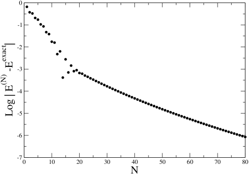
Figure 1: Logarithmic error for the energy for $g=-2$ as a function of $N$ for $\alpha=1/\sqrt{2}$

We first consider the asymptotic value $\alpha=1/\sqrt{2}$. Fig. 1 shows that $L_{N}$ decreases rapidly with $N$ when $N<\approx 20$ and then more slowly but more smoothly for $N>20$. In the transition region about $N\approx 20$ we observe oscillations that can mislead one into believing that the AIM starts to diverge.

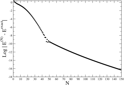
Figure 2: Logarithmic error for the energy for $g=-2$ as a function of $N$ for an almost optimal value $\alpha=1/2$

Fig. 2 shows that the behaviour of $L_{N}$ for a nearly optimal value $\alpha=1/2$ is similar to the previous case, except that the transition takes place at a larger value of $N$ and the convergence rate is greater. More precisely, $L_{N}$ decreases rapidly with $N$ when $N<\approx 50$ approximately as $L_{N}\approx 0.22-0.064N-0.0029N^{2}$ and more slowly and smoothly for $N>50$ as $L_{N}\approx-6.5-0.068N$. Again, the transition region exhibits oscillations.

Table 1 shows the ground–state energies for $g=-2,-1,1,2$ and the corresponding nearly optimal values of $\alpha$. We estimated those eigenvalues from the sequences of AIM roots for $N=10$ through $N=80$. Notice that the optimal values of $\alpha$ in Table 1 depend on $g$ and do not agree with the asymptotic value $\alpha=\sqrt{1/2}$. Table 1 also shows that the AIM eigenvalues agree with those calculated by means of the RPM [9, 10] from sequences of determinants of dimension $D=2$ through $D=15$.

The rate of convergence also depends on the chosen value of $r$. The calculation of $L_{N}$ as a function of $\xi=r/r_{0}$ shows that $L_{N}(\xi)$ exhibits a minimum at $\xi_{N}$ and that $\xi_{N}$ increases with $N$ approximately as $\xi_{N}=0.435+0.005N$ (for $g=-2$). However, in order to keep the application of the AIM as simple as possible we just choose $r=r_{0}$ for all the calculations.

4 Alternative perturbation approaches

Barakat [5] first converted the radial Schrödinger equation (1) into another one for an anharmonic oscillator by means of the standard transformations $r=u^{2}$ and $\Phi(u)=u^{-1/2}\Psi(u^{2})$. Finally, he derived the Sturm–Liouville problem

$$f^{{}^{\prime\prime}}(u)+2\left(\frac{L+1}{u}-\alpha u^{3}\right)f^{\prime}(u)+\left(\epsilon u^{2}-8gu^{4}+8Z\right)f(u)=0,$$ (7)

where $L=2l+1/2$ and $\epsilon=8E-(2L+5)\alpha$, through factorization of the asymptotic behaviour of the solution:

$$\Phi(u)=u^{L+1}e^{-\alpha u^{2}/4}f(u),\;\alpha=\sqrt{8\lambda}.$$ (8)

Notice that present $\alpha$ and Barakat’s $\alpha$ are not exactly the same but they have a close meaning and are related by $\alpha_{asymptotic}^{present}=\alpha_{Barakat}/4$. Since Barakat’s application of the AIM to Eq. (7) did not appear to converge [5] he opted for a perturbation approach that consists of rewriting Eq. (7) as

$$f^{{}^{\prime\prime}}(u)+2\left(\frac{L+1}{u}-\alpha u^{3}\right)f^{\prime}(u)+\left[\epsilon u^{2}+\gamma\left(-8gu^{4}+8Z\right)\right]f(u)=0$$ (9)

and expanding the solutions in powers of $\gamma$:

$$f(u)=\sum_{j=0}^{\infty}f^{(j)}(u)\gamma^{j},\;\epsilon=\sum_{j=0}^{\infty}\epsilon^{(j)}\gamma^{j}$$ (10)

The perturbation parameter $\gamma$ is set equal to unity at the end of the calculation. The series for the energy exhibits considerable convergence rate and consequently Barakat obtained quite accurate results with just two to five perturbation corrections [5]. Barakat calculated the coefficient $\epsilon^{(0)}$ exactly and all the others approximately [5].

The model (1) is suitable for several alternative implementations of perturbation theory in which we simply write $V(r)=V_{0}(r)+\gamma V_{1}(r)$ and expand the solutions in powers of $\gamma$.

If we choose $V_{0}(r)=-Z/r$ (when $Z>0$) and $V_{1}(r)=gr+\lambda r^{2}$ then we can calculate all the perturbation coefficients exactly by means of well known algorithms [8]. One easily realizes that the perturbation series can be rearranged as

$$E=Z^{2}\sum_{i=0}^{\infty}\sum_{j=0}^{\infty}d_{ij}g^{i}\lambda^{j}Z^{-(3i+4j)}.$$ (11)

It is well known that this series is asymptotic divergent for all values of the potential parameters.

The other reasonable perturbation split of the potential energy is $V_{0}(r)=\lambda r^{2}$, $V_{1}(r)=-Z/r+gr$. In this case we can rearrange the series as

$$E=\lambda^{1/2}\sum_{i=0}^{\infty}\sum_{j=0}^{\infty}c_{ij}Z^{i}g^{j}\lambda^{-(i+3j)/4}.$$ (12)

One expects that this series has a finite radius of convergence. This is exactly the series obtained by Barakat [5] by means of the AIM and, consequently, it is not surprising that he derived accurate results from it. In this case one can obtain exact perturbation corrections at least for the first two energy coefficients.

For simplicity we concentrate on the states with $n=0$. The eigenfunctions and eigenvalues of order zero are

$$\Psi_{0l}^{(0)}(r) = \frac{\sqrt{2}(2\lambda)^{(2l+3)/8}}{\Gamma(l+3/2)}r^{l+1}e^{-\sqrt{2\lambda}r^{2}/2}$$

$$E_{0l}^{(0)} = \frac{\sqrt{2\lambda}}{2}(2l+3)$$ (13)

respectively. With the unperturbed eigenfunctions one easily obtains the perturbation correction of first order to the energy

$$E_{0l}^{(1)}=\frac{(l+1)!g}{(2\lambda)^{1/4}\Gamma(l+3/2)}-\frac{l!Z(2\lambda)^{1/4}}{\Gamma(l+3/2)}$$ (14)

that is the term of the series (12) with $i+j=1$. One can easily carry out the same calculation for the states with $n>0$ using the appropriate eigenfunctions of the harmonic oscillator.

Equation (14) yields all the numerical results for $\epsilon_{0l}^{(1)}$ in Tables 1-3 of Barakat’s paper [5]. In particular, $E_{0l}^{(1)}=0$ when $g=\sqrt{2\lambda}Z/(l+1)$ as in Table 1 of Barakat’s paper [5]. This particular relationship between the potential parameters also leads to exact solutions of the eigenvalue equation (1). Some of them are given by

$$\Psi_{0l}^{exact}(r) = N_{l}r^{l+1}e^{-\alpha r^{2}-\beta r},\;\alpha=\sqrt{\frac{\lambda}{2}},\;\beta=\frac{Z}{l+1},$$

$$E_{0l}^{exact} = \alpha(2l+3)-\frac{Z^{2}}{2(l+1)^{2}},\;g=\frac{\sqrt{2\lambda}Z}{l+1},$$ (15)

where $N_{l}$ is a normalization constant.

5 Conclusions

We have shown that the AIM converges for the perturbed Coulomb model if the values of the free parameters in the factor function that converts the Schrödinger equation into a Sturm–Liouville one are not too far from optimal. It is clear that it is not necessary to transform the perturbed Coulomb model into an anharmonic oscillator for a successful application of the AIM. Our results do not exhibit the oscillatory divergence reported by Barakat[5] even when choosing the asymptotic value of $\alpha$.

The perturbation approach proposed by Barakat [5] is equivalent to choosing the harmonic oscillator as unperturbed or reference Hamiltonian, and if we apply perturbation theory to the original radial Schrödinger equation we easily obtain two energy coefficients exactly instead of just only one. It is worth mentioning that the coefficients calculated by Barakat [5] are quite accurate and, consequently, the resulting series provide a suitable approach for the eigenvalues of the perturbed Coulomb potential. This application of the AIM to perturbation theory is certainly much more practical than the calculation of exact perturbation corrections proposed earlier [7] that can certainly be carried out more efficiently by other approaches [8].

Acknowledgements

P.A. acknowledges support from Conacyt grant C01-40633/A-1

Table 1: Energies for some $g$ values calculated by the AIM with $N=80$ and RPM [9, 10] with $D=15$

$g$	$\alpha$	AIM	RPM
-2	0.5	$-1.17167358472$	$-1.1716735847197$
-1	0.3	$-0.226186875190871929$	$-0.2261868751908719$
1	0.3	$1.33284549226484083$	$1.3328454922648408349$
2	0.5	$2.014906226463$	$2.0149062264617370560$

References

- [1] Ciftci H, Hall R L, and Saad N 2003 J. Phys. A 36 11807.
- [2] Fernández F M 2004 J. Phys. A 37 6173.
- [3] Ciftci H, Hall R L, and Saad N 2005 J. Phys. A 38 1147.
- [4] Barakat T 2005 Phys. Lett. A 344 411.
- [5] Barakat T 2006 J. Phys. A 39 823.
- [6] Barakat T, Abodayeh K, and Mukheimer A 2005 J. Phys. A 38 1299.
- [7] Ciftci H, Hall R L, and Saad N 2005 Phys. Lett. A 340 388.
- [8] Fernández F M 2000 Introduction to Perturbation Theory in Quantum Mechanics (CRC Press, Boca Raton).
- [9] Fernández F M 1995 J. Phys. A 28 4043.
- [10] Fernández F M 1996 J. Phys. A 29 3167.