Reply to M. Ziman’s “Notes on optimality of direct characterization of quantum dynamics”

Abstract

Recently M. Ziman MarioNote06 criticized our approach for quantifying the required physical resources in the theory of Direct Characterization of Quantum Dynamics (DCQD) MohseniLidar06 in comparison to other quantum process tomography (QPT) schemes. Here we argue that Ziman’s comments regarding optimality, quantumness, and the novelty of DCQD are inaccurate. Specifically, we demonstrate that DCQD is optimal with respect to both the required number of experimental configurations and the number of possible outcomes over all known QPT schemes in the $2^{2n}$ dimensional Hilbert space of $n$ system and $n$ ancilla qubits. Moreover, we show DCQD is more efficient than all known QPT schemes in the sense of overall required number of quantum operations. Furthermore, we argue that DCQD is a new method for characterizing quantum dynamics and cannot be considered merely as a subclass of previously known QPT schemes.

I
Reply to the first comment: Quantification of resources

In general, for a non-trace preserving completely positive (CP) quantum dynamical map acting on a $d$ dimensional quantum system, the number of independent elements to be characterized is exactly $d^{4}$ Nielsen:book . In fact, in many important physical situations the quantum dynamical maps are effectively non-trace preserving. This phenomenon usually appears either as loss for photonic systems (due to inherent imperfections of optical elements), or leakage for atomic and spin-based quantum systems (due to interactions with photonic and/or phononic environments, spin-orbital coupling, etc.). Therefore, Ziman’s statement, “Each quantum device acting on a $d$ dimensional quantum system is described by $d^{4}-d^{2}$ independent parameters that has to be specified in arbitrary (complete) process tomography scheme.” MarioNote06  is not completely accurate. Even though one can always consider a larger Hilbert space such that the map becomes trace-preserving, this mathematical trick has little or no physical/practical significance, since in general we do not have full control over such an extended space. I.e., we cannot arbitrarily redefine our system and its environment in real life cases.

In Ref. MohseniLidar06 we only compared our Direct Characterization of Quantum Dynamics (DCQD) scheme with separable quantum process tomography (QPT) methods, including standard quantum process tomography (SQPT) Nielsen:book and the separable AAPT DAriano01 . Ziman raises the possibility of using non-separable QPT methods and proposed new resource quantification tables (the second and third tables in Ref. MarioNote06 ). As we argue below in a detailed analysis of such schemes, these tables are, unfortunately, incomplete and/or inaccurate.

In general, the required state tomography in AAPT could also be realized by non-separable quantum measurements. These measurements can be performed either: (1) in the same Hilbert space, such as mutually unbiased bases (MUB) measurements Wooters:89 ; LawrenceMUB02 , or (2) in a larger Hilbert space, such as a generalized measurement or POVM DArianoUQO02 . However, we find that these types of measurements would hardly have any practical relevance in the context of QPT, because they require many-body interactions that are not experimentally available. In the next two subsections we address each of these two approaches separately.

I.1 AAPT with Mutual Unbiased Bases Measurements

The AAPT scheme utilizes the degrees of freedom of an auxiliary system, $B$, in order to characterize an unknown quantum dynamical map acting on a principle system $A$. The information about the dynamics is obtained by complete quantum state tomography of the combined system and ancilla. Quantum state tomography in itself is the task of characterizing an unknown quantum state by measuring the expectation values of a set of non-commuting observables on the subensemble of quantum systems prepared in the same state. For characterizing the density operator of a $d$-dimensional quantum system, there are in general $d^{2}-1$ non-commuting observables to be measured. The minimal number of non-commuting measurements, that corresponds to a mutually unbiased basis, is $d+1$ (for systems with $d$ being a prime or a power of prime) Wooters:89 ; LawrenceMUB02 . A set of bases, in a given Hilbert space, are mutually unbiased if the inner products of each pair of elements in these bases have the same magnitude.

Let us consider the case of characterizing a non-trace preserving dynamical map acting on a single qubit $A$, using a single ancilla qubit $B$. For such a two-qubit system $d=4$, and the number of MUB for the required state tomography is five. Therefore, the minimum number of ensemble measurements (experimental configurations) in the AAPT scheme in a single qubit case is five, (as opposed to four mentioned in Ref. MarioNote06 ). The first measurement provides four independent outcomes and the last four measurements each provide three independent outcomes. I.e., we have, $1\times[(1\times 4)+(4\times 3)]=16$, where in each term in the sum the first number ($1,4$) represents the number of required measurements per input state, and the second number ($4,3$) represents the number of outcomes for each measurement; $16$ corresponds to the total number of independent outcomes. This should be compared with $4\times(1\times 4)=16$  in the DCQD scheme MohseniLidar06 . The first number ($4$) is the number of required different input states (compared to $1$ in the AAPT scheme).

It should be noted that if we know the local state of the ancilla (i.e., if we know the results of the measurements $I^{A}\otimes I^{B}$, $I^{A}\otimes\sigma_{x}^{B}$, $I^{A}\otimes\sigma_{y}^{B}$ and $I^{A}\otimes\sigma_{z}^{B}$ from our prior knowledge about the preparation and the fact that the output state has trace unity), then we need to find only $d^{4}-d^{2}$ parameters for the superoperator. But even in this case, we still need five different measurement setups. For a simple proof, let us examine the MUB of a two-qubit system, see the table in Fig.1 (also Ref. LawrenceMUB02 ). Obviously, for a non-trace preserving map we need at least five (ensemble) measurements corresponding to each row (measuring simultaneously the commuting operators in the first two columns). Now the question is, how many measurements are needed if we already know the local state of the ancilla? The answer becomes clear if we note that the measurements $I^{A}\otimes\sigma_{x}^{B}$, $I^{A}\otimes\sigma_{y}^{B}$, and $I^{A}\otimes\sigma_{z}^{B}$ appear in the second column of the first three rows and are redundant. However, we still need to perform all three (ensemble) measurements corresponding to the first three rows, since the measurements in the first column (corresponding to the local state of the principal qubit 1 – $\sigma_{x}^{A}\otimes I^{B}$, $\sigma_{y}^{A}\otimes I^{B}$ and $\sigma_{y}^{A}\otimes I^{B}$) do not commute. These three measurements plus the two measurements related to the 4th and 5th rows (corresponding to measuring the correlations of the principal qubit and the ancilla) result in five measurements overall. Note that the above argument is independent of the basis chosen, since in any other basis the measurements corresponding to the local state of the ancilla always appear in different rows due to the non-commuting properties of the Pauli operators.

Figure 1: A mutually unbiased basis (MUB) of the $4$-dimensional Hilbert space of the principal qubit $(A)$ and its ancilla $(B)$. Each row represents a different experimental configuration.

For the case of $n$ qubits, and by using $n$ ancillary qubits, the required measurements for the AAPT scheme can be performed using three different types of methods: (a) using $16^{n}$ (separable) joint single-qubit measurements on the $n$ principal and $n$ ancillary qubits, or (b) using $5^{n}$ mutually unbiased bases measurements (tensor product of MUB measurements on two-qubit systems), or more efficiently (c) using $4^{n}+1$ (non-separable) mutually unbiased bases measurements on the Hilbert space of all $2n$ qubits. The latter method requires many-body interactions between all $2n$ qubits, which are obviously not naturally available. The required global Hamiltonian can be written as $H=\sum\limits_{i=1}^{2n}O_{i}=\sum\limits_{i=1}^{2n}\bigotimes\limits_{k=1}^{2n}\sigma_{\alpha(i,k)}^{k}$, where $[O_{i},O_{j}]=0$ for any $i,j\in\{1,2,\ldots,2n\}$, such that their common eigenvectors form a MUB, and $\sigma_{\alpha(i,k)}^{k}$ is a Pauli operator ($\sigma_{x}^{k}$, $\sigma_{y}^{k}$ or $\sigma_{z}^{k}$) acting on the $k^{\mathrm{th}}$ qubit. I.e. one should simultaneously measures $2n$ commuting Hermitian operators $O_{i}\in\{O_{1},O_{2},...O_{2n}\}$; each operator $O_{i}$ in itself acts on $2n$ physical qubits as $O_{i=\{\alpha_{1},\alpha_{2},\alpha_{3,.}..\}}=\sigma_{\alpha_{1}}^{1}\sigma_{\alpha_{2}}^{2}\sigma_{\alpha_{3}}^{3}...\sigma_{\alpha_{2n}}^{2n}$ (e.g., for the case of three qubits see Fig. 2 of Ref. LawrenceMUB02 ).

The operators $O_{i}$ and $O_{j}$ commute globally and are made of tensor products of Pauli operators, however they cannot be simultaneously measured locally, i.e. by using only single-qubit devices. The reason is that according to the Heisenberg uncertainty principle, the outcome of each local measurement $\sigma_{\alpha}^{k}$ for the operator $O_{i}$ completely destroys the outcome of measuring $\sigma_{\beta}^{k}\neq\sigma_{\alpha}^{k}$ for other operators $O_{j}$. In principle, one could simulate the required many-body interactions in AAPT (for each of the $4^{n}+1$ measurements) by a quantum circuit comprising about $O(n^{2})$ single and two-qubit quantum operations (with the assumption of realizability of non-local two-body interactions, i.e., with having access to two-qubit interactions between every pairs of the $2n$ qubit system) MRL06 . For a simple proof, we note that the measurement of an operator in the form $\sigma_{z}^{1}\sigma_{z}^{2}\sigma_{z}^{3}...\sigma_{z}^{2n}$ requires $2n$ sequential CNOT operations. For measuring a more general operator of the form $O_{i=\{\alpha_{1},\alpha_{2},\alpha_{3,.}..\}}=\sigma_{\alpha_{1}}^{1}\sigma_{\alpha_{2}}^{2}\sigma_{\alpha_{3}}^{3}...\sigma_{\alpha_{2n}}^{2n}$, we need an additional $O(n)$ local single qubit operations to make an appropriate change of basis. Therefore, for measuring $2n$ operators $O_{i}$, one at least needs to realize $(2n)^{2}$ quantum operations. However, if only local two-body interactions are available (i.e., if we are restricted to using nearest neighbor interactions) then $O(n^{3})$ single- and two-body quantum operations would be required. The reason is that the overall number of operations grows by a factor of $O(n)$ due to the cost of transporting each two-qubit gate. A modified table for comparing physical resources in different QPT methods is presented in Fig. 2.

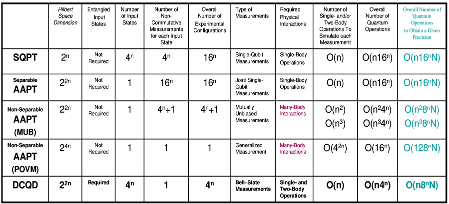
Figure 2: Comparison of the required physical resources for characterizing an arbitrary non-trace preserving CP quantum dynamical map on $n$ qubits. The overall number of experimental configurations (5th column) is obtained from multiplying the number of required input states and the number of non-commuting measurements at the output states. In principle, the required many-body interactions for AAPT+MUB can be simulated by a quantum circuit comprising about $O(n^{2})$ [$O(n^{3})$] single and two-qubit quantum operations with the assumption of non-local [local] two-body interactions. However, the many-body interactions for a POVM in this context cannot be efficiently simulated. The overall number of quantum operations (9th column) is defined as the product of the number of experimental configurations and the number of single- and/or two-body operations required for simulating each measurement. Finally, the overall number of quantum operations for a desired precision is obtained by multiplying by a factor of $2^{(k-1)n}N$ the 9th column, where $2^{kn}$ is the number of possible outcomes in each QPT strategy, and $N$ is the number of repeated measurements to obtain the precision $\epsilon\sim\frac{1}{\sqrt{N/2^{kn}}}$. We note that DCQD is more efficient than all known QPT schemes with respect to the overall number of quantum operations (see 9th and 10th columns).

Note that the AAPT plus MUB measurements with $O(n^{2})$ [or $O(n^{3})$] two-body interactions is essentially in the same complexity class as a quantum Fourier transform. This should be compared to the DCQD scheme with a single step of $n$ CNOT (between each qubit and its ancilla) and $n$ Hadamard operations to realize a single Bell-state measurement. In the context of estimating quantum dynamics, the implementation of $O(n^{2})$ or $O(n^{3})$ gates in AAPT is inefficient, since these operations not only increase the time execution of each measurement, they also create additional errors that would be very difficult to discriminate from the actual quantum dynamical map. Moreover, the overall number of repetitions for these operations scales poorly with a given desired precision.

Although MUB is not the most general measurement for state tomography of a $2n$-qubit system, it is well-understood (for systems whose dimensions is a power of prime) to be the optimal measurement scheme for such a task. Therefore, any other measurement strategy within the same Hilbert space results in more ensemble measurements than MUB. For other systems (whose dimensions is not a power of prime) the scaling of the AAPT measurements becomes even worse; since in those systems, the existence and construction of MUB is not fully understood and therefore in general one has to measure a complete operator basis of $2n$-qubit system which has $2^{4n}-1$ members.

In principle, one could devise intermediate strategies for AAPT, using different combinations of single-, two-, and many-body measurements. The number of measurements in such methods ranges from $4^{n}+1$ to $16^{n}$, which is always larger than what is required in DCQD MohseniLidar06 , using $4^{n}$ Bell-state measurements. Therefore, in the $2^{2n}$ dimensional Hilbert space of the $2n$ system and ancillary qubits, DCQD requires fewer experimental configurations than all other QPT schemes.

Using DCQD one can in principle transfer $\log_{2}2^{2n}$ bits of classical information between two parties, Alice and Bob, which is optimal according to the Holevo bound HolevoBound . Alice can realize this task by encoding a string of $2^{2n}$ bits of classical information into a(n) (engineered) quantum dynamics (e.g., by applying one of $2^{2n}$ unitary operator basis to the $n$ qubits in her possession and then send them to Bob). Bob can decode the message by a single measurement on $2n$ qubits using DQQD scheme MohseniLidar06 . I.e., the overall number of possible independent outcomes in each measurement in DCQD is $2^{2n}$, which is exactly equal to the number of independent degrees of freedoms for a $2n$ qubit system, therefore, a maximum amount of information can be extracted in each measurement in DCQD, which cannot be improved by any other possible QPT strategies in the same Hilbert space.

I.2 AAPT with Generalized Measurements

In principle, it is possible to perform the required quantum state tomography at the output states of an AAPT scheme by utilizing a single POVM or generalized measurement DArianoUQO02 . However, for characterizing the dynamics on $n$ qubits the number of required ancillary qubits should be increased from $n$ to $3n$ (see Fig. 3. of Ref DArianoUQO02 ). This can be easily understood according to the Holevo bound. For extracting complete information about a quantum dynamical map (encoded by $2^{4n}$ independent parameters of the superoperator) in a single measurement, one needs a Hilbert space of dimension at least $2^{4n}$; otherwise the Holevo bound cannot be satisfied. There are two major disadvantages of using such a POVM compared to all other QPT schemes. (1) The POVM measurement requires a general many-body interaction between $2n$ qubits that cannot be efficiently simulated. I.e., it requires an exponential number of single- and two-qubits quantum operations. (2) The number of required repetition of each measurement to obtain a desired precision grows exponentially with $n$.

According to the general setting in Ref. DArianoUQO02 , in order to implement a POVM for extracting all the information about any observable of an $n$-qubit system, one needs to realize a global normal operator $\mathsf{H}$ (a single universal quantum observable) in the Hilbert-Schmidt space of the principle system and an ancilla system in the form of $\mathsf{H}=\sum_{i=1}^{2^{2n}}E_{i}\otimes P_{i}$. Here $[\mathsf{H},\mathsf{H}^{\dagger}]=0$, $\left\{E_{i}\right\}$ is an operator basis for the $n$-qubit Hilbert space of the system, and $\left\{P_{i}\right\}$ is a set of projections over the ancilla Hilbert space (e.g., $P_{i}=|i\rangle\langle i|$, where $\{|i\rangle\}$ is an orthonormal basis in the ancillary Hilbert space). The operator $\mathsf{H}$ has the most general form of an operator-Schmidt decomposition Nielsen and cannot be simulated in a polynomial number of steps. It is known that in general at least $O(4^{2n})$ single- and two-qubit operations are needed to simulate such general many-body operations acting on $2n$ qubits Vivek04 (see also Nielsen for different measures of complexity of a given quantum dynamics).

One important disadvantage of all QPT schemes in a larger Hilbert space (that rely on calculating $2^{kn}$ different joint probability distributions) is that each measurement has to be repeated by a factor $2^{(k-1)n}$ in order to build the same statistics as a SQPT scheme. Let us consider an implementation of SQPT with a desired precision of $\epsilon\sim\frac{1}{\sqrt{N}}$ in characterizing parameters of a superoperator, where $\epsilon$ represents the standard deviation and $N$  is the number of repeated measurements. Since each measurement in SQPT has $2^{n}$ possible outcomes, the precision $\epsilon$ can be obtained by $N=\frac{2^{n}}{\epsilon^{2}}$ measurements. Note that in order to obtain a similar statistical error $\epsilon$ with other methods of QPT, with $2^{kn}$ possible outcomes, we need to perform $N^{\prime}=2^{(k-1)n}N$ measurements for each experimental configuration. Therefore, the actual number of measurements for a POVM strategy, with $2^{4n}$ possible outcomes, grows by a factor of $2^{3n}$ with respect to SQPT and $2^{2n}$ with respect to DCQD – see the last column of the table in Fig. 2. We note that the overall number of quantum operations is still optimal for DCQD for any desired precision.

II Reply to the second comment: Independence from AAPT and usage of quantumness

Here, we argue that the DCQD scheme is an independent algorithm from the AAPT scheme. First, we note that DCQD has a different scaling from the AAPT scheme in the sense of the overall number of experimental configurations, or similar scaling while using only two-body interactions compared to many-body interactions in the non-separable AAPT. Clearly, such results could not have been obtained if DCQD were merely a subclass of AAPT.

Second, the required input states for DCQD must be entangled, which is in complete contrast to AAPT, where entanglement is not required at the input level. E.g., for characterizing quantum dynamical populations MohseniLidar06 , the input state in DCQD must be maximally entangled in order to form a nondegenerate stabilizer state (with two independent stabilizer generators). This follows from the quantum Hamming bound, according to which only nondegenerate stabilizer states can be utilized for obtaining full information about the nature of all $2^{2}$ different error operator basis elements, acting on a single qubit of a two-qubit system Nielsen:book . For characterizing quantum dynamical coherence, the entanglement in input states is absolutely necessary, for otherwise the expectation values of the normalizers always vanish and therefore do not provide any information about the dynamics. In addition, the error-detection measurements in DCQD (e.g., $Z^{A}Z^{B}$, $X^{A}Z^{B}$) are fundamentally non-separable, which is again in contrast to AAPT which also can be performed by joint single-qubit measurements.

Third, the DCQD method utilizes a different methodological approach to quantum dynamical characterization than the AAPT schemes. DCQD utilizes a set of entangled  input states and provides the set of commuting observables to maximize the amount of classical information about the dynamics, $\log_{2}d^{2},$ that can be obtained at each output state (according to the Holevo bound), without completely characterizing any of the output states. However, AAPT utilizes a single faithful (not necessary entangled) input state and provides the minimal set of non-commuting observables that should be measured in order to completely characterize the output state of the combined system and ancilla, and the amount of classical information that can be obtain in each measurement, $\log_{2}(d^{2}-1)$, is less than the maximum allowable according to the Holevo bound ($\log_{2}d^{2}$). Therefore, there cannot be any direct correspondence between DCQD and AAPT in any fixed Hilbert space of the system and ancilla. We believe that the only true similarity between AAPT and DCQD is the fact that both methods utilize the degrees of freedoms of an auxiliary system.

III Reply to the third comment: Direct characterization of dynamics

In order to remove any ambiguity, we would like to define what we mean by direct characterization of quantum dynamics. We define a QPT method to be a direct method if it satisfies these two conditions: (1) It should not rely on complete state tomography of the output states. (2) Each experimental outcome (joint probability distribution of observables) give direct information about either a single element of the superoperator, ($\chi_{mm}$) or a specific known subset of the superoperator’s elements (e.g., $\chi_{mm},\chi_{nn},\text{Re}(\chi_{mn})$).

AAPT is not a direct method because it does not satisfy the condition (1). One could argue that when the local state of the ancilla is known ($d^{2}$ parameters), only $d^{4}-d^{2}$ additional parameters must be characterized. However, since in this case one eventually also has access to $d^{4}$ parameters ($d^{2}$ of which were known from the beginning, the rest measured), this should clearly also count as complete state tomography

IV Conclusion

We agree that demonstrating an absolute advantage of one QPT scheme over the other QPT methods requires a complete quantification of the complexity of the preparations and measurements procedures. Indeed, we present a more detailed analysis in a separate publication MRL06 . In conclusion, we believe the following statements are true:

1. DCQD is a quantum algorithm for complete and direct characterization of quantum dynamics, which does not require state tomography.

2. We have proved that DCQD is optimal in the sense of both the required number of experimental configurations and the number of possible outcomes, over all other known QPT schemes in a given Hilbert space.

3. DCQD is quadratically more efficient than all separable QPT schemes in the number of experimental configurations.

4. A similar scale-up in the number of experimental configurations is achievable with the AAPT scheme and MUB measurements only if many-body interactions are realized (or simulated with $O(n^{2})$ or $O(n^{3})$ single- and two-body gates).

5. In principle, by utilizing POVMs, a single experimental configuration is sufficient for a complete QPT, however, one should realize many-body interactions that are not experimentally available and cannot be efficiently simulated by single- and two-body interactions. Moreover, the POVM strategy has to be repeated as many as $4^{n}$ times more than DCQD to obtain a similar precision.

6. DCQD is new method for QPT, and cannot be considered merely as a subclass of any known QPT methods.

7. DCQD is the first theory that utilizes quantum error detection methods in quantum process tomography.

V Applications and future work

We believe that a potentially important advantage of DCQD is for use in partial characterization of quantum dynamics, where we cannot afford or do not need to carry out a full characterization of the quantum system under study, or when we have some a priori knowledge about the dynamics. We have already presented two examples in connection with simultaneous measurement of $T_{1}$ and $T_{2}$, and realization of generalized quantum dense coding tasks. Other implications and applications of DCQD remain to be investigated and explored, specifically, for obtaining a polynomial scale-up in physical resources for partial characterization of quantum dynamics. We believe that in some specific regimes DCQD could have near-term applications (within the next 5-10 years) for complete verification of small quantum information processing units (fewer than five qubits or so), especially in trapped-ion and liquid-state NMR systems. For example, the number of required experimental configurations for systems of 3 or 4 physical qubits is reduced from $5000$ and $65000$ (in SQPT) to $64$ and $256$, respectively, in our scheme. Complete characterization of such dynamics would be essential for verification of quantum key distribution procedures, teleportation units (in both quantum communication and scalable quantum computation), quantum repeaters, quantum error correction procedures, and more generally, in any situation in quantum physics where a few qudits have a common local bath and interact with each other. Another interesting extension of DCQD is to develop a theory for closed-loop and continuous characterization of quantum dynamics by utilizing weak measurements for our error-detection procedures.

This work was supported by the Natural Sciences and Engineering Research Council of Canada (to M.M. and D.A.L.), DARPA-QuIST, and the Sloan Foundation (to D.A.L). We thank M. Ziman for inspiring us to more carefully consider the resource requirements in our DCQD scheme and other known QPT schemes, and also acknowledge many useful discussions with A. T. Rezakhani.

References

- (1) M. Ziman, Notes on optimality of direct characterization of quantum dynamics, quant-ph/0603151.
- (2) M. Mohseni and D. A. Lidar, Direct characterization of quantum dynamics: I. General theory, quant-ph/0601033, Direct characterization of quantum dynamics: II. Detailed analysis, quant-ph/0601034.
- (3) M. A. Nielsen and I. L. Chuang, Quantum Computation and Quantum Information (Cambridge University Press, Cambridge, UK, 2001).
- (4) G. M. D’Ariano and P. Lo Presti, Phys. Rev. Lett. 86, 4195 (2001).
- (5) W. K. Wootters and B. D. Fields, Ann. Phys. 191, 363 (1989).
- (6) J. Lawrence, C. Brukner, Phys, Rev. A. 65, 032320 (2002).
- (7) G. M. D’Ariano, Phys. Lett. A 300, 1 (2002).
- (8) M. Mohseni, A. T. Rezakhani, and D. A. Lidar, in preparation (2006).
- (9) A. S. Holevo, Probl. Infor. Transm. 9, 110 (1973).
- (10) M. A. Nielsen et al., Phys. Rev. A 67, 052301 (2003).
- (11) V. V. Shende et al., Phys. Rev. A 69, 062321 (2004); M. Möttönen et al., Phys. Rev. Lett. 93, 130502 (2004).