Artificial Decoherence and its Suppression
in NMR Quantum Computer

Abstract

Liquid-state NMR quantum computer has demonstrated the possibility of quantum computation and supported its development. Using NMR quantum computer techniques, we observed phase decoherence under two kinds of artificial noise fields; one a noise with a long period, and the other with shorter random period. The first one models decoherence in a quantum channel while the second one models transverse relaxation. We demonstrated that the bang-bang control suppresses decoherence in both cases.

I Introduction

Quantum computation currently attracts a lot of attention since it is expected to solve some of computationally hard problems for a conventional digital computer ref:1 . Numerous realizations of a quantum computer have been proposed to date. Among others, a liquid-state NMR (nuclear magnetic resonance) quantum computer is regarded as most successful. Demonstration of Shor’s factorization algorithm VSB01 is one of the most remarkable achievements.

Although the current liquid-state NMR quantum computer is suspected not to be a true quantum computer because of its poor spin polarization at room temperature pt , it still works as a test bench of a working quantum computer. Following this concept, we have demonstrated experimentally using an NMR quantum computer that some of theoretical proposals really work qaa ; warp . In this contribution, we will show that a liquid-state NMR quantum computer can model not only a quantum computer but also the composite system of a quantum computer and its environment. Therefore, one can employ it to test the effectiveness of proposed decoherence control methods, such as a bang-bang control bb ; uchiyama . Note that the decoherence control methods are usually difficult to be tested because of extremely short coherence time in the real system.

II Decoherence

Decoherence is a phenomenon in which a quantum system undergoes irreversible change through its interaction with the environment. This is analyzed using the total Hamiltonian

$$H_{\rm t}=H_{\rm s}+H_{\rm e}+H_{\rm se},$$ (1)

where $H_{\rm s}$ and $H_{\rm e}$, in the absence of $H_{\rm se}$, determine the system and the environment behavior, respectively. On the other hand, $H_{\rm se}$ determines the interaction between the system and the environment. See, Fig. 1. Zurek discussed a simplified model where a two-level system (the system) is coupled to $n$ two-level systems (the environment) through $\sigma_{z}\otimes\sigma_{z}$ type interaction zurek .

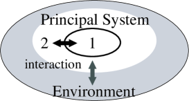
Figure 1: System and environment. The system consists of subsystems 1 and 2.

II.1 Artificial Decoherence

If the effect of $H_{\rm se}$ is small enough to be ignored compared with those of $H_{\rm s}$ and $H_{\rm e}$ in a certain time scale $\tau$, $H_{\rm s}$ can be considered as

$$H_{\rm s}=H_{1}+H_{2}+H_{12}.$$ (2)

$H_{1}$ and $H_{2}$, if $H_{12}$ does not exist, determine the behavior of subsystem 1 and 2, respectively, while $H_{12}$ determines the interaction between the subsystems. See, Fig. 1. Therefore, we may regard the subsystem 1 (2) as the system (environment) in the time scale $\tau$ and that the dynamics of the subsystem 1 can model that of a certain system. Zhang et al. experimentally studied the behavior of ¹³C-labeled trichloroethane, which has three spins, using NMR techniques zhang and claimed that they studied the decoherence.

We, however, note that a large number of degrees of freedom of the subsystem 2 is necessary to observe a decoherence-like behavior in the subsystem 1. This condition is not satisfied with molecules employed in liquid-state NMR quantum computation. If the degrees of freedom of the subsystem 2 is small, a periodic behavior in the subsystem 1 should be observed instead of an irreversible one. Teklemariam et al. introduced a stochastic classical field which is acting on the subsystem 2 in order to overcome the limitation of the model caused by the small degrees of the freedom of the subsystem 2 Teklemariam . The approach by Teklemariam et al. can be considered as a generation of random noise on the subsystem 1 through the subsystem 2 by applying a stochastic classical field to the subsystem 2.

II.2 Artificial Decoherence in One-Qubit

Let us consider a molecule containing two spins (qubits) as a system. The first qubit is regarded as the subsystem 1 and the second qubit as the subsystem 2. The Hamiltonian, when an individual rotating frame is assigned to each qubit, is

$$H_{\rm s} = JI_{z}\otimes I_{z},$$ (3)

where $I_{k}=\sigma_{k}/2$ and $\sigma_{k}$ is the $k$-th Pauli matrix. Note that $H_{1}=H_{2}=0$ in this rotating frame. We take a series of $\pi$-pulses acting on the second qubit as a classical field introduced by Teklemariam et al. Teklemariam . We create a pseudo-pure state $|00\rangle$ before starting experiments. Therefore, the Hamiltonian (3) is equivalent with

$$H_{\rm s} = J(t)\,I_{z}.$$ (4)

The spin operator $I_{z}$ appeared in Eq. (4) denotes the spin of the subsystem 1, while $|J(t)|=J$ and its sign changes when the $\pi$-pulse acts on the spin 2. We assume that the duration of a $\pi$-pulses is infinitely short. Therefore, we can model “a system containing one qubit in a time dependent field”, where the field strength is constant but its sign changes in time (telegraphic).

A stochastic classical field is, here, a series of $\pi$-pulses acting on the second qubit randomly in time.

III Experimental set-up

A 0.6 ml, 200 mM sample of ¹³C-labeled chloroform (Cambridge Isotope) in d-6 acetone is employed as a two-qubit molecule and data is taken at room temperature with a JEOL ECA-500 NMR spectrometer, whose hydrogen Larmor frequency is approximately 500 MHz jeol . The measured spin-spin coupling constant is $J/2\pi=215.5$ Hz and the transverse relaxation time is $T_{2}\sim 7.5$ s for the hydrogen nucleus (subsystem 2) and $T_{2}\sim 0.30$ s for the carbon nucleus (subsystem 1). The longitudinal relaxation time is measured to be $T_{1}\sim 20$ s for both nuclei. The duration of a $\pi$-pulses for both nuclei is set to $50~{}\mu$s.

III.1 Decoherence in Channel

Let us consider a flying qubit traveling in a channel, as a first example. It is assumed that there exists a noise source on a certain position in the channel, which causes decoherence in the flying qubit.

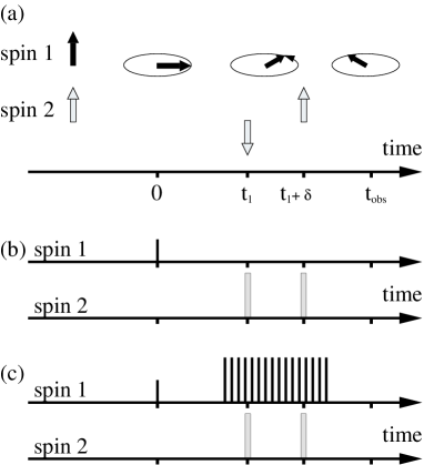
Figure 2: Model of “decoherence in a channel”. (a) The dynamics of the spins is schematically shown. The spin 1 rotates in the $xy$-plane with the angular velocity $-J/2$ except between $t=t_{1}$ and $t=t_{1}+\delta$, during which the angular velocity is $J/2$. The spin 2 is flipped at $t=t_{1}$ and $t=t_{1}+\delta$. The FID signal of the spin 1 is measured at $t=t_{m}$. (b) The pulse sequences for realizing the spin dynamics shown in (a). The short bar indicates a $\pi/2$-pulse acting on the spin 1, while the long squares are $\pi$-pulses acting on the spin 2. (c) Pulse sequences compensating the “decoherence” obtained in (b). The 16 long bars are $\pi$-pulses acting on the spin 1 with the interval of 0.3 ms.

In order to model the above case, we performed an experiment schematically shown in Fig. 2. The pseudopure state $|00\rangle$ (or, $|\!\!\uparrow\uparrow\rangle$) is prepared by the field gradient method pps . A $\pi/2$-pulse acts on the spin 1 at $t=0$. Then, the spin 1 is turned into the $x$-axis in the rotating frame and starts rotating in the $xy$-plane with an angular velocity $-J/2$. A pair of $\pi$-pulses are applied to the spin 2 at $t=t_{1}$ and $t_{1}+\delta$ and then the spin 1 rotates with the angular velocity $J/2$ during this period. The FID (free induction decay) signal at $t=t_{m}$ is measured and shown as the open square in Fig. 3 (a). The $x$- ($y$-) component is the real (imaginary) component of the FID signal. The signal is normalized so that the data point should be on the point $(1,0)$ when $\delta=0$. Note that open squares are on a circle of unit radius, but with different phases because of different duration $\delta$. We randomly choose 128 $\delta$s between 0 and $2\pi/J$ and average FID signals, as shown in Fig. 3 (a). Averaging over all signals gives a smaller averaged FID signal than that of each FID signal, which indicates that decoherence occurred because of the noise source in the channel.

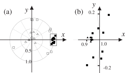
Figure 3: Experimental results of “decoherence in a channel”. The FID signals measured at $t=t_{m}$ in Fig. 2 are shown in the $xy$- (real and imaginary)-plane. The solid and open symbols are with and without the decoherence suppression pulses shown in Fig. 2 (c). (a) The open squares denote the first 8 FID signals without averaging. The 8 open triangles denote the averaged FID signals over 16 experiments. The open circle near the origin denotes the averaged value of all ($16\times 8=128$) the FID signals. The region marked by the rectangle is enlarged in (b). (b) The solid squares denote the first 8 FID signals without averaging. The 8 solid triangles denote the averaged FID signals over 16 results. The solid square on the $x$-axis shows the averaged value of all (128) the FID signals.

Kitajima, Ban, and Shibata discussed a method to suppress the above decoherence kitajima . They argued that a series of $\pi$-pulses acting on the spin 1, while the spin 1 is under the influence of the noise source, should suppresses the above decoherence. Their idea is essentially the same as the field inhomogeneity compensation using the spin echo method spin_echo . Figure 2 (c) shows the pulse sequence realizing their decoherence suppression proposal. Since we do not know the exact position of the noise source in advance, we apply many (16 here) $\pi$-pulses to the spin 1. If a noise source exists within this period (equivalently, region when the flying qubit is really moving) of the 16 $\pi$-pulses, the effect of the noise is greatly suppressed. We observed this behavior in our experiments, as shown in Fig. 3 (c). The amplitude of each FID signals are the same and the variation of the phases in the $xy$-plane is remarkably decreased as shown in Fig. 3 (c). Therefore, it is clearly seen that decoherence is greatly suppressed.

III.2 Transverse Relaxation

Let us model a phenomenon called a transverse relaxation next. Suppose that there is a spin in a magnetic field $(0,0,B_{0})$. The spin points the $z$-direction in thermal equilibrium. Then, let us turn the spin in the $xy$-plane by a $\pi/2$-pulse. The spin starts rotating in the $xy$-plane with the angular velocity $\omega_{0}=\gamma B_{0}$, where $\gamma$ is the gyromagnetic ratio of the spin. This spin rotation is called a precession and can be observed as a FID signal in NMR. If there is no relaxation mechanism, it precesses forever and thus the FID signal does not decay in time. The transverse relaxation is a phenomena that the spin is still in the $xy$-plane but its FID signal decreases in time. The transverse relaxation is modeled, in the simplest case, as a random walk process rwa ; bb on the circle shown in Fig. 3 (a).

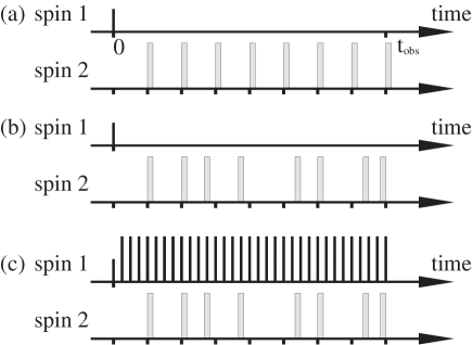
Figure 4: Pulse sequences for modeling “transverse relaxation”. The pseudopure state $|00\rangle$ is prepared first. The spin 1 is turned into the $x$-axis by the $\pi/2$-pulse at $t=0$. (a) The pulse sequence provides a reference. A series of the $\pi$-pulses acts on the spin 2. The interval of the pulses is fixed to $\Delta=2$ ms. The sequence shown here yields the solid squares in Fig. 5. (b) The pulse sequences to realize the artificial transverse relaxation. The intervals between the pulses are randomly modulated. See, the text. The artificial transverse relaxation is obtained by averaging over various (128) series of $\pi$-pulses on the spin 2. (c) The pulse sequence for realizing the bang-bang control. In addition to the pulse sequence shown in (b), $\pi$-pulses act on the spin 1, of which intervals are $0.5$ ms $<\Delta$.

We performed an experiment schematically shown in Fig. 4. The pseudopure state $|00\rangle$ is prepared by the field gradient method pps . A $\pi/2$-pulse is applied to the spin 1 at $t=0$. Then, the spin 1 is turned into the $x$-axis in the rotating frame and starts rotating with an angular velocity $J$. The pulse sequence shown in Fig. 4 (a) provides a reference, which is necessary because the intrinsic relaxation cannot be avoided in the experiments. The FID signal is measured at $t=t_{m}$ after a series of $\pi$-pulses acting on the spin 2, of which interval is fixed to $\Delta=2$ ms here. Note that the number of the $\pi$-pulses on the spin 2 determines the period while the spin 1 is under the influence of time dependent field, see Eq. (4). The amplitudes of the FID signals with various periods are shown as the solid squares. When we obtain a faster relaxation than this reference, then we can claim that the artificial relaxation is realized.

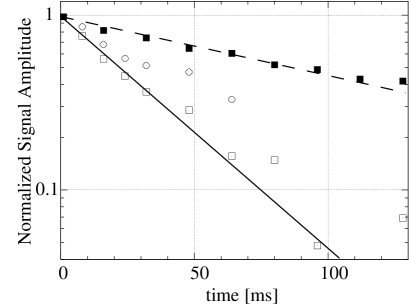
Figure 5: Experimental results demonstrating artificial “transverse relaxation” and its suppression. The solid squares show the amplitude of the FID signals of the spin 1 while the $\pi$-pulses are acting on the spin 2 every 2 ms. Those provide a reference for the other experimental results. The open squares show the amplitude of the averaged FID signals of the spin 1. We averaged 128 FID signals with various random series of $\pi$-pulses acting on the spin 2, here. The open circles show the amplitude of the averaged FID signals as in the case of the open squares but with the “bang-bang” control. The broken (solid) line is the least square fit of a function $e^{-t/T_{2}}$ and $T_{2}=128\,(33)$ ms to the solid (open) squares.

The artificial transverse relaxation is realized with the pulse sequence shown in Fig. 4 (b). In contrast to (a), the intervals between the pulses are randomly modulated as $\Delta(1+\alpha\,N_{D})$, where $\alpha$ is a parameter defining the strength of the relaxation and $N_{D}$ is a variable which obeys the normal distribution. We set $\alpha=0.25$ in Fig. 5. The artificial transverse relaxation is observed when the FID signals with various (128 in this experiment) series of $\pi$-pulses on the spin 2 are averaged. The open squares in Fig. 5 show the amplitudes of the averaged FID signals with various periods. We observe that the relaxation is faster than the reference case.

The pulse sequence to realize the bang-bang control bb ; uchiyama is shown in Fig. 4 (c). In addition to the pulse sequence shown in Fig. 4 (b), regular $\pi$-pulses act on the spin 1, of which intervals are $0.5$ ms $<\Delta=2$ ms. The relaxation with the bang-bang control is clearly smaller than that without it, as shown in Fig. 5. Therefore, we conclude that the effectiveness of the bang-bang control is confirmed.

The experimental results, when the parameter $\alpha$ is changed, is shown in Fig. 6. Note that the strength of the relaxation can be controlled by changing the parameter $\alpha$. We suspect that there is a non-Markovian behavior (non-exponential decay of the amplitude of the FID signal) when $\alpha=0.10$. We plan to investigate this behavior further in near future.

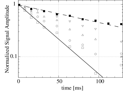
Figure 6: Experimental results demonstrating artificial “transverse relaxation” with various $\alpha$ values. The open squares, open circles, open triangles, and inverted open triangles show the results with $\alpha=0.25,0.20,0.15,0.10$, respectively. The solid squares show the reference as in Fig. 5.

IV Conclusion

We generated artificial decoherence (relaxations) using liquid-state NMR quantum computer techniques. The first type of decoherence takes place in a quantum channel, while the other is a transverse relaxation. Then, the bang-bang control is applied to the qubit which carries a quantum information and we confirmed that it indeed suppresses the two types of decoherence. Moreover, we have shown that the nature of the decoherence can be controlled by changing parameters.

The artificial decoherence thus generated is still simple, but we can extend our approach further. We believe that well controlled artificial decoherence will help to understand various types of decoherence in the real world and to develop methods to overcome them towards physical realization of a working quantum computer.

Extended version of this article with detailed theoretical analysis is in progress and reported elsewhere cv .

References

- (1) M. A. Nielsen and I. L. Chuang, Quantum Computation and Quantum Information (Cambridge University Press, Cambridge, 2000).
- (2) L. M. K. Vandersypen, M. Steffen, G. Breyta, C. S. Yannonl, M. H. Sherwood, and I. L. Chuang, Nature 414, 883 (2001).
- (3) R. Fitzgerald, Physics Today, 53 No. 1 (2000) 20.
- (4) M. Nakahara, Y. Kondo, K. Hata, and S. Tanimura, Phys. Rev. A 70, 052319 (2004).
- (5) M. Nakahara, J. J. Vartiainen, Y. Kondo, S. Tanimura, K. Hata, Phys. Lett. A 350, 27 (2006).
- (6) See, for example, H. Gutmann, F. K. Wilhelm, W. M. Kaminsky, and S. Lloyd, Bang-Bang Refocusing of a Qubit Exposed to Telegraph Noise in Experimental Aspects of Quantum Computing, edited by H. O. Everitt (Springer, New York, 2005).
- (7) C. Uchiyama and M. Aihara, Phys. Rev. A 66, 032313 (2002), C. Uchiyama and M. Aihara, Phys. Rev. A 68, 052302 (2003).
- (8) W. H. Zurek, Phys. Rev. D 8, 1862 (1982).
- (9) J. Zhang, Z. Lu, L. Shan, and Z. Deng, arXiv:quant-ph/0202146, J. Zhang, Z. Lu, L. Shan, and Z. Deng, arXiv:quant-ph/0204113.
- (10) G. Teklemariam ,E. M. Fortunato, C. C. L opez, J. Emerson, J. P, Paz, T. F. Havel, D. G. Cory Phys. Rev. A 67, 062316 (2003).
- (11) http://www.jeol.co.jp/, http://www.jeol.com/.
- (12) U. Sakaguchi, H. Ozawa, and T. Fukumi, Phys. Rev. A 61, 042313 (2000).
- (13) S. Kitajima, M. Ban, and F. Shibata, No. 25aYG12 in the 60th annual meeting of the Physical Society of Japan (2005).
- (14) M. H. Levitt, Spin Dynamics, (John Wiley and Sons, New York, 2001).
- (15) D. Pines and C. P. Slichter, Phys. Rev. 100, 1014 (1955).
- (16) Y. Kondo, M. Nakahara, S. Tanimura, S. Kitajima, C. Uchiyama, and F. Shibata, in preparation.