Voronoi Diagrams for Pure 1-qubit Quantum States

Abstract

1-qubit quantum states form a space called the three-dimensional Bloch ball. To compute Holevo capacity, Voronoi diagrams in the Bloch ball with respect to the quantum divergence have been used as a powerful tool. These diagrams basically treat mixed quantum states corresponding to points in the interior of the Bloch ball. Due to the existence of logarithm in the quantum divergence, the diagrams are not defined on pure quantum states corresponding to points on the two-dimensional sphere. This paper first defines the Voronoi diagrams for pure quantum states on the Bloch sphere by the Fubini-Study distance and the Bures distance. We also introduce other Voronoi diagrams on the sphere obtained by taking a limit of Voronoi diagrams for mixed quantum states by the quantum divergences in the Bloch ball. These diagrams are shown to be equivalent to the ordinary Voronoi diagram on the sphere.

1 Introduction

Quantum information has been attracting computer scientists as a new computing paradigm [7]. To develop a sound theory for handling such quantum information, we need to understand the structure of quantum information from the viewpoint of information processing. Some aspect of quantum information is to define a kind of distance between two quantum states. Depending on the specific applications in quantum estimation [5], quantum information geometry [1], quantum channel capacity [3], etc., there are many quantum distances, each having meanings in some respective settings.

Voronoi diagrams have been playing a central role to represent the proximity relation of point set, etc., with a wide variety of applications in many fields. It is quite natural to investigate the proximity relation via Voronoi diagrams of quantum states with respect to such distances.

Using the Voronoi diagrams of mixed quantum states with respect to the quantum divergence, Oto, Imai and Imai [11] introduced a method to calculate Holevo capacity. Since there are many kinds of distances between quantum states, we expect that a similar method can be applicable to investigations of other distances. In addition, to investigate the difference between some two different distances of quantum states, to see if their Voronoi diagrams coincide or not can be a good first approach. However, the Voronoi diagrams used in [11] are not defined on pure quantum states. Therefore, it is reasonable to investigate if the Voronoi diagrams used there can be extended to pure states. In 1-qubit case, pure states correspond to the surface of Bloch ball, and mixed states to the interior. Geometrically, the problem can be express as “Can the Voronoi diagram defined only in the interior of the Bloch ball be extended to its surface?”

Moreover, even from other points of view, pure quantum states are quite important and useful. For example, most quantum algorithms have been described using only pure states without using mixed states even if some measurements are performed during the algorithm and quantum states are then better to be treated as mixed ones.

In this paper, we first explain the method to calculate Holevo capacity. This method uses Voronoi diagrams for mixed quantum states by the quantum divergence. Secondly, we define Voronoi diagrams for pure quantum states on the Bloch sphere by the Fubini-Study distance and the Bures distance. These diagrams are shown to be equivalent to the ordinary Voronoi diagram on the sphere. We also introduce other Voronoi diagrams on the sphere which are obtained by taking a limit of the Voronoi diagrams used in the calculation of Holevo capacity. Finally, all these diagrams — the one by the Fubini-Study distance, the one by the Bures distance, and the one obtained by taking a limit of the diagram in mixed states — are shown to be identical.

Consequently, as far as the proximity relation among 1-qubit pure states are uniquely defined for these distances and divergences, it may be regarded to be natural in a sense that geometric structures of pure states are nicer than those of mixed states.

2 Preliminaries

2.1 Bures distance and Fubini-Study distance

A 1-qubit quantum state is represented by a density matrix $\rho$:

$$\rho=\frac{1}{2}\left(\begin{array}[]{cc}1+z&x-{\rm i}y\\ x+{\rm i}y&1-z\end{array}\right),\qquad x^{2}+y^{2}+z^{2}\leq 1.$$

$\rho=\rho(x,y,z)$ may be identified with a point $(x,y,z)$ in the 3-dimensional space, and a ball formed by all such points

$$B=\{\,(x,y,z)\mid x^{2}+y^{2}+z^{2}\leq 1\}$$

is called Bloch ball. A state with rank 1 is called pure, while a state with rank 2 is called mixed. Points on the boundary of the Bloch ball, i.e., the Bloch sphere, corresponds to pure states.

For two pure states $\rho$ and $\sigma$, the Fubini-Study distance $d_{\rm FS}(\rho,\sigma)$ is defined by

$$\cos d_{\rm FS}(\rho,\sigma)=\sqrt{{\rm Tr}\;(\rho\sigma)},\qquad 0\leq d_{\rm FS}(\rho,\sigma)\leq\frac{\pi}{2}.$$

See Hayashi [4]. The Bures distance $d_{\rm B}(\rho,\sigma)$ [2] is defined by

$$d_{\rm B}(\rho,\sigma)=\sqrt{1-{\rm Tr}\;(\rho\sigma)}.$$

2.2 Quantum divergence and Holevo capacity

Eigenvalues $\lambda_{1},\lambda_{2}$ of $\rho(x,y,z)$ are given by $(1\pm\sqrt{x^{2}+y^{2}+z^{2}})/2$. By the eigenvalue decomposition, $\rho$ can be expressed as $\rho=\sum_{i}\lambda_{i}E_{i},$ where $E_{i}E_{j}$ is $E_{i}$ for $i=j$ and is 0 for $i\not=j$. Then, for a mixed state $\rho(x,y,z)$, $\log\rho$ is defined by $\log\rho=\sum_{i}(\log\lambda_{i})E_{i}.$ In the Bloch ball, information-geometric structure can be induced by the von Neumann entropy $S(\rho)$ and the quantum divergence $D(\rho||\sigma)$. The von Neumann entropy of a state $\rho$ is defined by $S(\rho)={\rm Tr}\;(-\rho\log\rho).$ Using the eigenvalues $\lambda_{1},\lambda_{2}$ of $\rho$, it is expressed as $S(\rho)=-\sum_{i}\lambda_{i}\log\lambda_{i}$ i.e., $S(\rho)$ is the Shannon entropy of eigenvalues. Note that $0\log 0=0$. The quantum divergence $D(\rho||\sigma)$ for two quantum states $\rho$ and $\sigma$ is defined by

$$D(\rho||\sigma)={\rm Tr}\;(\rho(\log\rho-\log\sigma)).$$

where $\sigma$ is a mixed state. It is known that $D(\rho||\sigma)\geq 0$, and $D(\rho||\sigma)=0$ iff $\rho=\sigma$.

Now we consider the situation of sending a qubit via a quantum channel $\Gamma$ with noise and receiving it. A quantum channel means that $\Gamma$ is a affine transformation that maps a quantum state to a quantum state. If $\rho(x,y,z)$ is 1-qubit quantum state, the image of $\Gamma$

$$\left\{(x^{\prime},y^{\prime},z^{\prime})\mid\rho^{\prime}(x^{\prime},y^{\prime},z^{\prime})=\Gamma(\rho(x,y,z)),(x,y,z)\in B\right\}$$

is an ellipsoid and included in the Bloch ball.

The Holevo capacity of this quantum channel is known to be equal to the maximum divergence from the center to a given point and the radius of the smallest enclosing ball. The Holevo capacity $C(\Gamma)$ of a 1-qubit quantum channel $\Gamma$ is defined as

$$C(\Gamma)=\inf_{\theta}\sup_{\rho}D(\Gamma(\rho)||\Gamma(\theta)),\qquad(\theta,\rho\in B).$$

3 Computing the Holevo capacity of 1-qubit Quantum Channel

The method to compute the Holevo capacity of a 1-qubit quantum channel is described in [11]. There, the Voronoi diagrams of 1-qubit mixed states by quantum divergence are used to solve the smallest enclosing ball problem. The Voronoi diagrams were introduced as a generalization of Kullback-Leibler divergence [8, 9]. In this section, we briefly explain the process of computation and its mathematical background.

We plot sufficiently many points $V=\left\{v_{1},v_{2},\ldots,v_{N}\right\}$ on the sphere and consider the Voronoi diagram of the points $\Gamma(V)$ with respect to the divergence. If $\#V$ is large enough, we can assume that the radius of the smallest enclosing ball of the points $\Gamma(V)$ sufficiently approximates the real value of the Holevo capacity. To compute the smallest enclosing ball, Voronoi diagrams are considered as a useful tool. Two Voronoi diagrams used here are defined as

$$V_{D}(v_{i})=\bigcap_{i\neq j}\left\{\sigma|D(\sigma||\rho(v_{i}))\geq D(\sigma||\rho(v_{j}))\right\},$$

$$V_{D^{*}}(v_{i})=\bigcap_{i\neq j}\left\{\sigma|D(\rho(v_{i})||\sigma)\geq D(\rho(v_{j})||\sigma)\right\}.$$

Although our concern is primarily $V_{D^{*}}$, we first consider $V_{D}$ because it is easier to compute. Actually, considering the graph of $w=-S(\rho(x,y,z))=\phi(x,y,z)$, $D(\rho(x,y,z)||\sigma(\tilde{x},\tilde{y},\tilde{z}))$ corresponds to the distance along w-axis between the tangent plain at $(\tilde{x},\tilde{y},\tilde{z})$ and the point $(x,y,z)$ (Fig. 2). This fact makes it easy to compute the $V_{D}$ using a lower envelope of the tangent plains (Fig. 2).

Then, we compute $V_{D^{*}}$ as a dual diagram of $V_{D}$. To solve the problem, we consider a dual coordinate system $\rho^{*}(u,v,w)$ corresponding to $\rho(x,y,z)$ such that $D(\rho||\sigma)=D^{*}(\sigma^{*}||\rho^{*})$. Their coordinate change is explicitly defined as

$$(u,v,w)\equiv\nabla\phi=\frac{1}{2}\left(\log\frac{1+r}{1-r}\right)\frac{1}{r}(x,y,z).$$

Thus, $V_{D^{*}}$ can be computed from $V_{D}$. In fact, this process to work out $V_{D^{*}}$ from $V_{D}$ can be extended to a general $d$-dimensional case [11]. Now using $V_{D^{*}}$, the center of the smallest enclosing ball is determined and finally we obtain approximate value of the Holevo capacity as the radius of the ball.

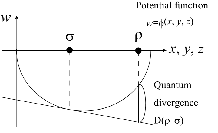
Figure 1: Geometric meaning of a divergence

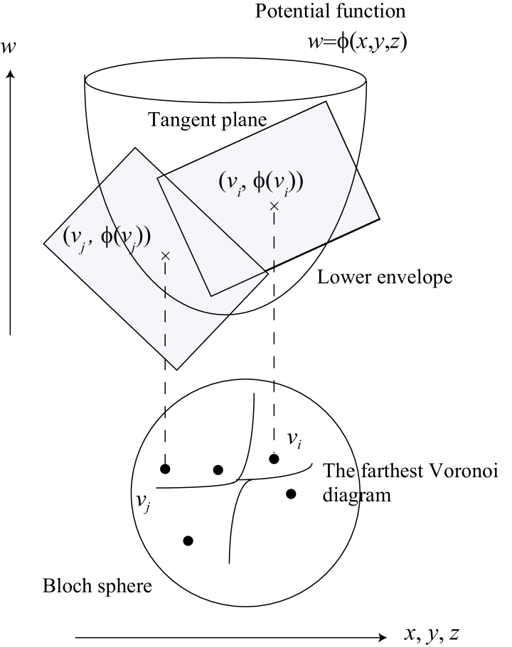
Figure 2: Computation of Voronoi diagram via a lower envelope

4 Voronoi diagram of 1-qubit pure states

We first consider the Fubini-Study distance $d_{\rm FS}(\rho,\sigma)$ for two 1-qubit pure states $\rho=\rho(x,y,z)$ and $\sigma=\sigma(\tilde{x},\tilde{y},\tilde{z})$ with $x^{2}+y^{2}+z^{2}=\tilde{x}^{2}+\tilde{y}^{2}+\tilde{z}^{2}=1$. First, we have

$${\rm Tr}\;(\rho\sigma)=\frac{1}{2}(1+x\tilde{x}+y\tilde{y}+z\tilde{z}).$$

Hence, setting $\theta(\rho,\sigma)$ to be an angle between two vectors $(x,y,z)$ and $(\tilde{x},\tilde{y},\tilde{z})$ with $0\leq\theta\leq\pi$, we have

$$d_{\rm FS}(\rho,\sigma)=\cos^{-1}\sqrt{(1+\cos\theta(\rho,\sigma))/2}=\theta(\rho,\sigma)/2.$$

In the 1-qubit case, the Fubini-Study distance between two pure states is a half of the geodetic distance between two corresponding points on the Bloch sphere.

Concerning the Bures distance,

$$d_{\rm B}(\rho,\sigma)=\sqrt{\frac{1}{2}(1-x\tilde{x}-y\tilde{y}-z\tilde{z}))}=\frac{1}{\sqrt{2}}d_{\rm E}((x,y,z),(\tilde{x},\tilde{y},\tilde{z}))$$

where $d_{\rm E}$ is the three-dimensional Euclidean distance.

Thus, at a first glance, these two distance might look strange, but in the 1-qubit case both are just natural distances. In fact, one we restrict discussions on pure states only, these are more direct consequences. However, the above formulation is suitable to connect it with mixed states. This point will be discussed in the concluding remarks.

Voronoi diagrams for pure 1-qubit states can be defined by using the Fubini-Study distance or the Bures distance. Suppose $n$ pure 1-qubit states $\sigma_{i}=\sigma(x_{i},y_{i},z_{i})$ $(i=1,\ldots,n)$ are given. Define $V_{\rm FS}(\sigma_{i})$ by

$$V_{\rm FS}(\sigma_{i})=\bigcap_{j\not=i}\{(x,y,z)\mid\rho=\rho(x,y,z)\colon\ \hbox{pure states},d_{\rm FS}(\rho,\sigma_{i})<d_{\rm FS}(\rho,\sigma_{j})\}$$

which is the Voronoi region of $\sigma_{i}$ with respect to the Fubini-Study distance. Similarly, $V_{\rm B}(\sigma_{i})$ with respect to the Bures distance can be defined. Combining the above-mentioned discussions with results on the ordinary Voronoi diagrams on the sphere (e.g., [6]), we have the following.

Theorem 1

For $n$ 1-qubit pure states, the following four Voronoi diagrams are equivalent:

1. the Voronoi diagram with respect to the Fubini-Study distance

2. the Voronoi diagram with respect to the Bures distance

3. the Voronoi diagram on the sphere with respect to the ordinary geodetic distance

4. the section of the three-dimensional Euclidean Voronoi diagram with the sphere

5 Voronoi diagram of 1-qubit states by the quantum divergence

As described above, the Voronoi diagram of 1-qubit states with respect to the quantum divergence plays a very important roll in computation of Holevo capacity. So far, the Voronoi diagrams are defined only in mixed states. Actually, while $D(\rho||\sigma)={\rm Tr}\;\rho(\log\rho-\log\sigma)$ can be defined when an eigenvalue of $\rho$ equals $0$ because $0\log 0$ can be naturally defined as $0$, it is not defined when an eigenvalue of $\sigma$ is $0$. Here we show that this Voronoi diagram of mixed states can be extended to pure states. In other words, we prove that even though the divergence $D(\rho||\sigma)$ can not be defined when $\sigma$ is a pure state, the Voronoi edges are naturally extended to pure states. To prove this convergence, we revisit the geometric structure described in [11] by presenting explicit expressions.

For a 1-qubit state $\rho=\rho(x,y,z)$ with $r\equiv\sqrt{x^{2}+y^{2}+z^{2}}$, the eigenvalues of $\rho$ is given by

$$\lambda_{1}=\frac{1+r}{2},\qquad\lambda_{2}=\frac{1-r}{2}.$$

When $(x,y)\not=(0,0)$, defining a unitary matrix $U$ as

$$U=\frac{1}{\sqrt{2}}\left(\begin{array}[]{cc}\displaystyle{\frac{x-{\rm i}y}{\sqrt{x^{2}+y^{2}}}\sqrt{\frac{r+z}{r}}}&\displaystyle{\frac{x-{\rm i}y}{\sqrt{x^{2}+y^{2}}}\sqrt{\frac{r-z}{r}}}\vskip 12.0pt plus 4.0pt minus 4.0pt\\ \displaystyle\sqrt{\frac{r-z}{r}}&-\displaystyle\sqrt{\frac{r+z}{r}}\\ \end{array}\right),$$

$\rho$ is expressed as

$$\rho=U\left(\begin{array}[]{cc}\lambda_{1}&0\\ 0&\lambda_{2}\\ \end{array}\right)U^{*}.$$

Then,

$$\begin{array}[]{rl}\log\rho&={}\displaystyle{U\left(\begin{array}[]{cc}\log\lambda_{1}&0\\ 0&\log\lambda_{2}\\ \end{array}\right)U^{*}}\vskip 6.0pt plus 2.0pt minus 2.0pt\\ &={}\displaystyle{\frac{1}{2r}\left(\begin{array}[]{cc}(r+z)\log\lambda_{1}+(r-z)\log\lambda_{2}&(x-{\rm i}y)(\log\lambda_{1}-\log\lambda_{2})\vskip 3.0pt plus 1.0pt minus 1.0pt\\ (x+{\rm i}y))(\log\lambda_{1}-\log\lambda_{2})&(r-z)\log\lambda_{1}+(r+z)\log\lambda_{2}\\ \end{array}\right)}.\end{array}$$

For $\rho=\rho(x,y,z)$ and $\sigma=\sigma(\tilde{x},\tilde{y},\tilde{z})$ with $\tilde{r}=\sqrt{\tilde{x}^{2}+\tilde{y}^{2}+\tilde{z}^{2}}<1$, $\tilde{\lambda}_{1}=(1+\tilde{r})/2$, and $\tilde{\lambda}_{2}=(1-\tilde{r})/2$, we have the following:

$$\begin{array}[]{rcl}{\rm Tr}\;(\rho\log\sigma)&{}={}&\displaystyle\frac{1}{4\tilde{r}}(\log\tilde{\lambda}_{1}[(1+z)(\tilde{r}+\tilde{z})+2(x\tilde{x}+y\tilde{y})+(1-z)(\tilde{r}-\tilde{z})]\\ &&\qquad+\log\tilde{\lambda}_{2}[(1+z)(\tilde{r}-\tilde{z})-2(x\tilde{x}+y\tilde{y})+(1-z)(\tilde{r}+\tilde{z})]\\ &=&\displaystyle\frac{1}{2\tilde{r}}(\log\tilde{\lambda}_{1}[\tilde{r}+x\tilde{x}+y\tilde{y}+z\tilde{z}]+\log\tilde{\lambda}_{2}[\tilde{r}-x\tilde{x}-y\tilde{y}-z\tilde{z}])\vskip 3.0pt plus 1.0pt minus 1.0pt\\ &=&\displaystyle{\frac{1}{2}\log\frac{1-\tilde{r}^{2}}{4}+\frac{\log(1+\tilde{r})-\log(1-\tilde{r})}{2\tilde{r}}[x\tilde{x}+y\tilde{y}+z\tilde{z}]}.\\ \end{array}$$

When $\tilde{x}=\tilde{y}=0$ and $\tilde{z}\not=0$ for this $\sigma$, we have

$${\rm Tr}\;(\rho\log\sigma)=\frac{1+z}{2}\log\frac{1+\tilde{z}}{2}+\frac{1-z}{2}\log\frac{1-\tilde{z}}{2}=\frac{1}{2}\log\frac{1-\tilde{r}^{2}}{4}+\frac{\log(1+\tilde{r})-\log(1-\tilde{r})}{2\tilde{r}}z\tilde{z}$$

and we now have the following.

Lemma 1

For a 1-qubit mixed state $\sigma=\sigma(\tilde{x},\tilde{y},\tilde{z})$ with $(\tilde{x},\tilde{y},\tilde{z})\not=(0,0,0)$ and a general 1-qubit state $\rho=\rho(x,y,z)$,

$$D(\rho\|\sigma)={\rm Tr}\;(\rho\log\rho)-\frac{1}{2}\log\frac{1-\tilde{r}^{2}}{4}-\frac{\log(1+\tilde{r})-\log(1-\tilde{r})}{2\tilde{r}}[x\tilde{x}+y\tilde{y}+z\tilde{z}].$$

Moreover, $D(\rho||\sigma)$ converges to ${\rm Tr}\;(\rho\log\rho)-1/2\log 1/4$ as $(x,y,z)\rightarrow(0,0,0)$. This generalize the result and we can naturally assume that the above formula holds for all 1-qubit mixed states.

Now we revisit the Voronoi diagram defined by the quantum divergence. For a set of mixed states $\sigma^{\prime}_{i}=\sigma^{\prime}_{i}(x^{\prime}_{i},y^{\prime}_{i},z^{\prime}_{i})$ $(i=1,\ldots,n)$, we can define the Voronoi region $V_{D}(\rho_{i})$ of $\sigma_{i}$. Note that here $\sigma^{\prime}_{i}$ should be mixed, while $\rho$ can be pure. Suppose a set of pure states $\sigma_{i}=\sigma_{i}(x_{i},y_{i},z_{i})$ $(i=1,\ldots,n)$ is given. For a small $\epsilon>0$, consider the section of the Voronoi diagram of $\sigma^{\prime}_{i}(x^{\prime}_{i},y^{\prime}_{i},z^{\prime}_{i})$ defined by

$$(x^{\prime}_{i},y^{\prime}_{i},z^{\prime}_{i})=(1-\epsilon)(x_{i},y_{i},z_{i})$$

with a sphere of $x^{2}+y^{2}+z^{2}=(1-\epsilon)^{2}$. Define the Voronoi diagram $V_{D}$ of these given pure states for all pure states by the quantum divergence to be the limit of this section with $\epsilon\rightarrow 0$, and denote the Voronoi region of $\sigma_{i}$ in this diagram by $V_{D}^{\rm pure}(\sigma_{i})$.

Then, by using the above lemma, we have

$$V_{D}^{\rm pure}(\sigma_{i})=\bigcap_{j\not=i}\{(x,y,z)\mid\rho=\rho(x,y,z)\hbox{ on the Bloch sphere},\ x\tilde{x}_{i}+y\tilde{y}_{i}+z\tilde{z}_{i}\geq x\tilde{x}_{j}+y\tilde{y}_{j}+z\tilde{z}_{j}\}$$

and see that this diagram is identical with those in the previous section.

Similarly as above, we can define $V_{D^{*}}(\sigma_{i})$ for pure $\sigma_{i}$, where $\rho$ should be mixed. For the Voronoi diagram with respect to the dual divergence $D^{*}$, consider its section with a sphere of $x^{2}+y^{2}+z^{2}=(1-\epsilon)^{2}$, and define the Voronoi diagram $V_{D^{*}}^{\rm pure}$ of these given pure states to be the limit of this section with $\epsilon\rightarrow 0$. The same arguments with $V_{D}^{\rm pure}$ can be applied to this case, and we obtain the following.

Theorem 2

The Voronoi diagrams $V_{D}^{\rm pure}$ and $V_{D^{*}}^{\rm pure}$ for $n$ pure states on the Bloch sphere are identical to those diagrams in Theorem 1.

It should be noted that, for mixed states, the Voronoi diagrams $V_{D}$ and $V_{D^{*}}$ for the same set of quantum states are not identical in general [11].

6 Concluding Remarks

We have shown that in the 1-qubit case the Voronoi diagrams defined by various distances and divergences of a finite set of pure states for all pure states are all identical. This would also hold in the higher-dimensional case, which is left as an open problem.

Our investigations on pure states shed light on studying differences among Voronoi diagrams with respect to many distances and divergences. In fact, for pure quantum states, the Fubini-Study distance is a unique metric once an appropriate differential-geometric invariance is imposed, whereas for mixed quantum states there are so many metrics, such as SLD Fisher metric, RLD Fisher metric and Bogoljubov Fisher metric (e.g., see [5]), each having some meaningful implications in some settings. In the case of fundamental information theory and statistics, some relations between the Voronoi diagram by the Kullback-Leibler divergence and that by the hyperbolic distance on the upper half-plane are touched upon [8, 9, 10]. Investigating proximity relations induced by such metrics is also left as a future work.

References

- [1] S.-I. Amari and H. Nagaoka: Methods of Information Geometry. Translated from the 1993 Japanese original by Daishi Harada. Translations of Mathematical Monographs, 191. AMS, Oxford University Press, Oxford, 2000.
- [2] D. Bures: An Extension of Kakutani’s Theorem on Infinite Product Measures to the Tensor Product of Semifinite -Algebras. Trans. Amer. Math. Soc., Vol.135 (1969), pp.199–212.
- [3] A. S. Holevo: The Capacity of the Quantum Channel with General Signal States. IEEE Trans. Inf. Theory, Vol.44, No.1 (1998), pp.269–273.
- [4] M. Hayashi: Asymptotic Estimation Theory for a Finite-Dimensional Pure State Model. Journal of Physics A: Mathematical and General, Vol.31 (1998), pp.4633–4655.
- [5] M. Hayashi, ed.: Asymptotic Theory of Quantum Statistical Inference — Selected Papers. World Scientific, 2005.
- [6] H. Imai, S. Sumino, K. Imai: On the Complexity of Minimax Facility Location Problem on a Sphere (in Japanese). Transactions of the IEICE, Vol.J71-D, No.6 (June 1988), pp.1155–1158.
- [7] M. A. Nielsen and I. L. Chuang: Quantum Computation and Quantum Information. Cambridge University Press, 2000.
- [8] K. Onishi and H. Imai: Voronoi Diagram in Statistical Parametric Space by Kullback-Leibler Divergence. Proceedings of the 13th ACM Symposium on Computational Geometry, 1997, pp.463–465.
- [9] K. Onishi and H. Imai: Voronoi Diagrams for an Exponential Family of Probability Distributions in Information Geometry. Japan-Korea Joint Workshop on Algorithms and Computation, Fukuoka, 1997, pp.1–8.
- [10] K. Onishi and N. Takayama: Construction of Voronoi Diagram on the Upper Half-Plane. IEICE Trans. Fundamentals, Vol.E79-A, No.4 (1996), pp.533–539.
- [11] M. Oto, H. Imai and K. Imai: Computational Geometry on 1-qubit Quantum States. Proc. International Symposium on Voronoi Diagrams in Science and Engineering (VD 2004), Tokyo, 2004, pp.145–151.