Induced photon statistics in three-level lasers

Abstract

The statistical properties of three-level lasing are investigated theoretically. It is assumed that the three-level medium is coherently excited by another laser with an arbitrary photon statistics. It is proved that, under the specific conditions, the photon statistics of the three-level laser duplicate the photon statistics of the exciting laser. We call this phenomenon an induced photon statistics. We suggest to use this to analyze the statistical properties of a laser involved into a feedback process. Applying this laser for the coherent pump of a three-level laser, we can follow its photon statistics by means of direct following the three-level generation. In accordance with Ref. Milburn , we conclude that the feedback in itself is unable to generate the non-classical manifestation in the laser field.

I Introduction

The three-level laser is a unique source of a bright light, where the quantum peculiarities in the field are produced automatically without any supplementary efforts such as, for example, an establishment of a regular pump Ref. Golubev . For this source, the stabilizing mechanism was investigated in detail and this is connected exclusively with the non-linear behaviour of the three-level medium interacting with two coherent fields Ref. Ritsch .

At the same time there is another field manifestation more interesting for us here. In Ref. Rost , it was illustrated that, in three-level lasing, the photon statistics can turn out to be dependent on statistical properties of the other laser that is used for the coherent pump of the three-level medium. In the cited work, it was suggested to employ this phenomenon for an improvement of the quantum statistical parameters in the sub-Poissonian three-level generation.

We are going to consider some effect that is inexplicitly already contained in the formulas of Ref. Rost but was in no way accented there. We shall demonstrate here that it is possible to ensure the conditions when the photon statistics in three-level lasing are not only dependent but duplicate the one in the pump laser. We call this phenomenon induced photon statistics (IPS).

To our mind, the IPS is of our interest in itself as a fundamental. At the same time one can see, where this phenomenon could be applied. Really, for example, if there is a situation when the laser beam turns out to be inaccessible for direct testing, then you could follow its statistical properties by means of following three-level lasing. For that, you need only to apply your laser for the coherent excitation of the last and ensure the conditions for existing the IPS.

The laser beam can be inaccessible for the direct investigation by the quite different reasons. For example, as is known some frequency ranges are extremely hardly detected or the light beam from the laser involved into the feedback process is inaccessible too.

The case with the feedback is more interesting for us and we shall touch it here. This problem was widely considered in different scientific groups experimentally by Yammamoto, Fofanov, Mosalov Yammamoto ; Fofanov ; Mosalov and theoretically by Troshin, Wiseman, and Milburn Milburn ; Troshin . Everybody of them has fixed that the photocurrent noise from the laser in the feedback loop (FBL) can be reduced even below the quantum limit. This experimentally demonstrated effect has produced the determined hopes that we are able to obtain sub-Poissonian lasing by means of only the establishment of the acceptable feedback.

However there are reasons to think differently too. The point is that the observed noise reduction was easy explained not only within the framework of quantum electrodynamics but as well as the classical one. This can mean only that the observed experimentally reduction of the current noise in the FBL is in no way connected logically with the photon noise one. In order to make some conclusions relative to the photon flux in this case, it is not quite enough to follow only the photocurrent and some supplementary measuring procedures must be provided.

From our standpoint, the determined clarity was reached by Weisman and Milburn in Ref. Milburn . There the authors could insist that the feedback is unable to ensure conditions for the generation of the non-classical light. The conclusion was made on the basis of the very formal considerations. They have proved that if the internal dynamics of the cavity generate a light state that has a positive Glauber-Sudarshan P-function, this positivity survives under switching the feedback on.

We think that it would be useful to illustrate the same on the less formal level by applying any measuring procedure, on the basis of any mental experimental situation. One of the possible procedure, to our mind, could be connected with theIPS and we are going to consider this way below in this article.

This paper is organized as follows. In Sec. II, the three-level laser model and the observed signals are considered. In Sec. III, the quantum statistical theory of the joint system consisting of the three-level laser and the coherently exciting laser is presented. In Sec. IV, the conditions for existing theinduced photon statistics are found. In Sec. V, the phenomenon of theinduced photon statistics is applied for analysis of the laser radiation from laser in the feedback loop.

II Joint system of exciting and three-level lasers

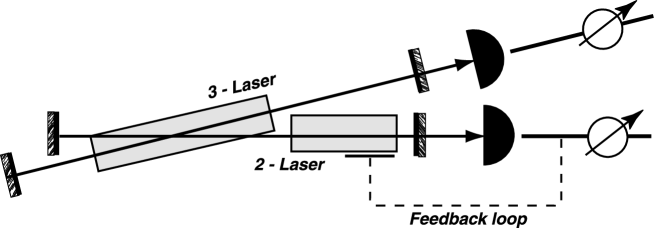
Figure 1: Mental experimental setup with two coupled lasers: ’2-laser’ is the two-level laser included into the feedback loop; ’3-laser’ is the three-level laser

We shall treat theoretically the same mental experiment as in Ref. Rost . One can see in Fig. 1 that there are two lasers interacting with each other by means of their common intracavity space. One of them is a two-level laser that is designated in the figure as ’2-laser’ (after (2L)). Its intracavity field is used for a coherent pump of a three-level laser (’3-laser’ in the figure or simply (3L)).

The feature of our theoretical approach to this experimental situation is of the same as in Ref. Rost . Usually, in the similar configurations, it is assumed that although the three-level medium is excited by the two-laser intracavity field, nevertheless this interaction does not affect on lasing itself. We are not going to be restricted by this assumption. On the contrary, the case when the main losses in the (2L) cavity are connected just with the three-level medium excitation is of our main interest here.

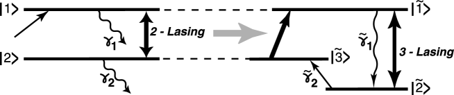
Figure 2: Atomic energetic configurations for the 2-laser (on the left) and the 3-laser (on the right)

In Fig. 2, both two- and three-level atomic configurations are shown together. We assume that the two-level medium (on the left in the figure) is pumped incoherently to the upper atomic state $|1\rangle$ with the mean rate $R$ and there are spontaneous decays of the atomic states $|1\rangle$ and $|2\rangle$ correspondingly with the rates $\gamma_{1}$ and $\gamma_{2}$.

It is supposed that three-level lasing takes place on the transition $|\tilde{1}\rangle\leftrightarrow|\tilde{2}\rangle$ (on the right in the figure). In order to ensure the (3L) generation, the three-level medium is excited coherently on the transition $|\tilde{3}\rangle\to|\tilde{1}\rangle$ by a radiation from the (2L) and incoherently on the transition $|\tilde{2}\rangle\to|\tilde{3}\rangle$ with the rate $\tilde{\gamma}_{2}$. Besides there is a spontaneous decay $|\tilde{1}\rangle\to|\tilde{2}\rangle$ with the rate $\tilde{\gamma}_{1}$. Hereinafter, the sign ’tilde’ over any symbol denotes that this symbol belongs to the (3L).

Let the output signals in our mental experiment be the photocurrent spectra $(\delta i^{2})_{\omega}$ and $(\delta\tilde{i}^{2})_{\omega}$ correspondingly for a registration of the (2L) and (3L) radiation. These spectra are defined as factors near the delta-functions in the pair correlation functions:

$$\overline{\delta i_{\omega}\;\delta i_{\omega^{\prime}}}=(\delta i^{2})_{\omega}\;\delta(\omega+\omega^{\prime}),\qquad\overline{\delta\tilde{i}_{\omega}\;\delta\tilde{i}_{\omega^{\prime}}}=(\delta\tilde{i}^{2})_{\omega}\;\delta(\omega+\omega^{\prime}).$$ (1)

The spectral components $\delta i_{\omega}$ and the photocurrent fluctuation $\delta i(t)=i(t)-\overline{i}$ are coupled by the Fourier transformation:

$$\delta i_{\omega}=\frac{1}{\sqrt{2\pi}}\int\limits_{-\infty}^{+\infty}\delta i(t)\;e^{i\omega t}dt,\qquad\delta i(t)=\frac{1}{\sqrt{2\pi}}\int\limits_{-\infty}^{+\infty}\delta i_{\omega}\;e^{-i\omega t}d\omega$$ (2)

and similarly for the other variable $\delta\tilde{i}_{\omega}$.

III Theory of the joint system of two lasers

III.1 Master equation

In the work Rost , the system of two lasers was considered within the framework of the master equation theory. The master equation was constructed in the Glauber diagonal representation in the limit of the high-Q cavity and the small photon fluctuations. the obtained master equation reads:

$$\frac{\partial R(\varepsilon,\tilde{\varepsilon},t)}{\partial t}=\frac{\partial}{\partial\varepsilon}\left((\kappa+\kappa_{0})\varepsilon-\tilde{\kappa}\tilde{\varepsilon}\right)R+\frac{\partial}{\partial\tilde{\varepsilon}}\left(2\tilde{\kappa}\tilde{\varepsilon}-\kappa_{0}\varepsilon\right)R+$$

$$+(\kappa+\kappa_{0})n\xi\frac{\partial^{2}R}{\partial\varepsilon^{2}}-\tilde{\kappa}\tilde{n}\frac{\partial^{2}R}{\partial\tilde{\varepsilon}^{2}}+\tilde{\kappa}\tilde{n}\frac{\partial^{2}R}{\partial\varepsilon\partial\tilde{\varepsilon}}+\{\cdots\}.$$ (3)

As is known, the Glauber field amplitude $\alpha=\sqrt{u}\;\exp(i\varphi)$ and $\tilde{\alpha}=\sqrt{\tilde{u}}\;\exp(i\tilde{\varphi})$ are introduced as eigen-numbers of the corresponding annihilation operators:

$$\hat{a}|\alpha\rangle=\alpha|\alpha\rangle,\qquad\hat{\tilde{a}}|\tilde{\alpha}\rangle=\tilde{\alpha}|\tilde{\alpha}\rangle,\qquad\left[\hat{a},\hat{a}^{\dagger}\right]=1,\qquad\left[\hat{\tilde{a}},\hat{\tilde{a}}^{\dagger}\right]=1.$$ (4)

The limit of the small photon fluctuations means that $\varepsilon=u-n$ and $\tilde{\varepsilon}=\tilde{u}-\tilde{n}$ turn out to be much less than the corresponding semi-classical meanings $n,\tilde{n}$:

$$\varepsilon\ll n,\qquad\tilde{\varepsilon}\ll\tilde{n}.$$ (5)

The photon matrix $R(\varepsilon,\tilde{\varepsilon},t)$ is introduced by the phase integrating the Glauber P-quasi-distribution:

$$R(\varepsilon,\tilde{\varepsilon},t)=\int\!\!\int d\varphi\;d\tilde{\varphi}\;P(\alpha,\tilde{\alpha},t).$$ (6)

The frequency parameters $\kappa$ and $\tilde{\kappa}$ are the spectral mode widths for the (2L) and the (3L);

$$\kappa_{0}=\tilde{\gamma}_{2}\;\left(\tilde{g}_{13}/\tilde{g}_{12}\right)^{2}\;\tilde{N}/\tilde{n}$$ (7)

is the mean rate of the coherent excitation of the three-level medium $\tilde{g}_{13}$ and $\tilde{g}_{12}$ are the coupling constants for the dipol interaction of the field with the three-level atom on the transitions $(1-3)$ and $(1-2)$, $\tilde{N}$ is the three-level atom number.

A statistical aspect of the 2L is determined by the arbitrary Mandel parameter $\xi$ that depends on statistical features of the pump of the laser medium. The last is determined by only parameter $p=-2\xi$ ($p<1$). By varying this parameter we can obtain the Poissonian ($p=0$), sub-Poissonian ($0<p<1$) or super-Poissonian ($p<0$) laser.

As for semiclassical solutions $n$ and $\tilde{n}$, the following useful equalities take place for them:

$$\tilde{\kappa}\tilde{n}=\kappa_{0}n\qquad(\kappa+\kappa_{0})n=R.$$ (8)

In order to simplify our formal expressions we have written all of them in the saturation regime relative to both lasers and taken the condition $\tilde{\gamma}_{2}\ll\tilde{\gamma}_{1}$. Also, it was assumed that there are no any non-linear manifestations in the coherent excitation of the three-level medium.

In the master equation, the notation $\{\cdots\}$ informs us that as a matter of fact there are the other terms containing the higher order derivatives with respect to $\varepsilon$ and $\tilde{\varepsilon}$. As is known we have no any possibility to avoid writing these terms in the case of the non-classical fields. However for the description of correlation experiments of the lowest orders, these terms nothing at all introduce.

III.2 Langevin equations

Let us rewrite our master equation theory in the terms of the corresponding differential Langevin equations for the variables $\varepsilon$ and $\tilde{\varepsilon}$:

$$\dot{\varepsilon}=-(\kappa+\kappa_{0})\varepsilon+\tilde{\kappa}\tilde{\varepsilon}+F(t),$$ (9)

$$\dot{\tilde{\varepsilon}}=-2\tilde{\kappa}\tilde{\varepsilon}+\kappa_{0}\varepsilon+\tilde{F}(t).$$ (10)

The pair correlation functions for the stochastic sources $F$ and $\tilde{F}$ are given by:

$$\overline{F(t)F(t^{\prime})}=2\xi(\kappa+\kappa_{0})n\;\delta(t-t^{\prime}),$$ (11)

$$\overline{\tilde{F}(t)\tilde{F}(t^{\prime})}=-2\tilde{\kappa}\tilde{n}\;\delta(t-t^{\prime}),$$ (12)

$$\overline{F(t)\tilde{F}(t^{\prime})}=\tilde{\kappa}\tilde{n}\;\delta(t-t^{\prime}).$$ (13)

The more complicated correlations are connected with terms $\{\cdots\}$ in master equation (3) and are not essential, because, in our consideration here, we are going to be restricted only by the pair correlations for the photon variables and we do not need to know the correlation function of the higher orders for stochastic sources.

In the c-number theory, the intracavity photon fluctuations are easy coupled with the corresponding photocurrent fluctuations $\delta i$ and $\delta\tilde{i}$ by means of the following equalities:

$$\delta i=\kappa\varepsilon+S(t),\qquad\overline{S(t)S(t^{\prime})}=\overline{i}\;\delta(t-t^{\prime}),\qquad\overline{i}=\kappa n,$$ (14)

$$\delta\tilde{i}=\tilde{\kappa}\tilde{\varepsilon}+\tilde{S}(t),\qquad\overline{\tilde{S}(t)\tilde{S}(t^{\prime})}=\overline{\tilde{i}}\;\delta(t-t^{\prime}),\qquad\overline{\tilde{i}}=\tilde{\kappa}\tilde{n}.$$ (15)

The stochastic sources here reflect the random process of the light absorption under detecting.

As was mentioned above, we are going to consider the photocurrent spectra as the signal in our mental experiment. One can see that the spectral components of the currents

$$\delta i_{\omega}=\kappa\varepsilon_{\omega}+S_{\omega},$$ (16)

$$\delta\tilde{i}_{\omega}=\tilde{\kappa}\tilde{\varepsilon}_{\omega}+\tilde{S}_{\omega}$$ (17)

are coupled directly with the spectral components $\varepsilon_{\omega}$ and $\tilde{\varepsilon}_{\omega}$. Thus it is better to rewrite equations (9) and (10) in the Fourier domain:

$$-i\omega\varepsilon_{\omega}=-(\kappa+\kappa_{0})\varepsilon_{\omega}+\tilde{\kappa}\tilde{\varepsilon}_{\omega}+F_{\omega},$$ (18)

$$-i\omega\tilde{\varepsilon}_{\omega}=-2\tilde{\kappa}\tilde{\varepsilon}_{\omega}+\kappa_{0}\varepsilon_{\omega}+\tilde{F}_{\omega}.$$ (19)

The corresponding pair correlation functions for the spectral stochastic sources read:

$$\overline{F_{\omega}F_{\omega^{\prime}}}=2\xi(\kappa+\kappa_{0})n\;\delta(\omega+\omega^{\prime}),\qquad\overline{\tilde{F}_{\omega}\tilde{F}_{\omega^{\prime}}}=-2\tilde{\kappa}\tilde{n}\;\delta(\omega+\omega^{\prime}),$$

$$\overline{F_{\omega}\tilde{F}_{\omega^{\prime}}}=\tilde{\kappa}\tilde{n}\;\delta(\omega+\omega^{\prime}),$$ (20)

$$\overline{S_{\omega}S_{\omega^{\prime}}}=\kappa n\;\delta(\omega+\omega^{\prime}),\qquad\overline{\tilde{S}_{\omega}\tilde{S}_{\omega^{\prime}}}=\tilde{\kappa}\tilde{n}\;\delta(\omega+\omega^{\prime}).$$ (21)

IV Photocurrent spectra

IV.1 General conditions

From algebraic Eqs. (18) and (19) it is not difficult to express the photon fluctuations via the stochastic sources in the following form:

$$\varepsilon_{\omega}=\frac{(2\tilde{\kappa}-i\omega)F_{\omega}+\tilde{\kappa}\tilde{F}_{\omega}}{(\kappa+\kappa_{0}-i\omega)(2\tilde{\kappa}-i\omega)-\kappa_{0}\tilde{\kappa}},$$ (22)

$$\tilde{\varepsilon}_{\omega}=\frac{\kappa_{0}F_{\omega}+(\kappa+\kappa_{0}-i\omega)\tilde{F}_{\omega}}{(\kappa+\kappa_{0}-i\omega)(2\tilde{\kappa}-i\omega)-\kappa_{0}\tilde{\kappa}}.$$ (23)

Now we have a possibility to calculate in the explicit form the photon spectral densities $(\varepsilon^{2})_{\omega}$ and $(\tilde{\varepsilon}^{2})_{\omega}$, i. e., the photocurrent spectra too. According to (16) and (17) the last are expressed via the first by:

$$(\delta\tilde{i}^{2})_{\omega}=\tilde{\kappa}^{2}(\tilde{\varepsilon}^{2})_{\omega}+(\tilde{S}^{2})_{\omega},$$ (24)

$$(\delta i^{2})_{\omega}=\kappa^{2}(\varepsilon^{2})_{\omega}+(S^{2})_{\omega}.$$ (25)

After the non-complicated algebraic manipulations, one can obtain the photocurrent in the (3L)-channel in the form:

$$(\delta\tilde{i}^{2})_{\omega}/\overline{\tilde{i}}=1-2\tilde{\kappa}^{2}\frac{\omega^{2}+(\kappa+\kappa_{0})(\kappa-\kappa_{0}\xi)}{\left(\omega^{2}-\tilde{\kappa}(2\kappa+\kappa_{0})\right)^{2}+\omega^{2}\left(2\tilde{\kappa}+\kappa+\kappa_{0}\right)^{2}},$$ (26)

and in the (2L)-channel:

$$(\delta i^{2})_{\omega}/\overline{i}=1+2\kappa\frac{\kappa_{0}\tilde{\kappa}^{2}+\xi(\kappa+\kappa_{0})(\omega^{2}+4\tilde{\kappa}^{2})}{\left(\omega^{2}-\tilde{\kappa}(2\kappa+\kappa_{0})\right)^{2}+\omega^{2}\left(2\tilde{\kappa}+\kappa+\kappa_{0}\right)^{2}}.$$ (27)

These spectra are obtained for the arbitrary relations between the frequency parameters $\kappa,\;\tilde{\kappa}$, and $\kappa_{0}$

Generally speaking, both spectra turn out to be dependent on the parameter $\xi$, i. e., on the photon statistics exciting laser.

IV.2 Spectra in the (2L)-channel

First of all, let us check what the photon statistics take place from the isolated (without the three-level medium) (2L). We remember that photocurrent (27) determines the photon statistics in the presence of three-level lasing that can seriously affects on the (2L). In order to obtain the required spectrum for the isolated laser, we must to put in Eq. (27) first $\kappa_{0}=0$ and second $\tilde{\kappa}=0$. A sense of the first requirement is very clear because just the coefficient $\kappa_{0}$ determines the connection between lasers. The second requirement is connected with equality (8) that as $\kappa_{0}=0$ survives only if $\tilde{n}=0$ or $\tilde{\kappa}=0$. Because under the construction of the master equation (3) in Ref. Rost we have employed the limit of the small photon fluctuations or equivalently $\tilde{n}\gg 1$.

So putting in (27) $\tilde{\kappa},\kappa=0$, the photocurrent spectrum for the isolated (2L) reads:

$$(\delta i^{2})_{\omega}/\overline{i}=1+2\xi\frac{\kappa^{2}}{\omega^{2}+\kappa^{2}}.$$ (28)

One can see that the photon statistics of the isolated (2L) is dependent on the statistical Mandel parameter $\xi$ and can be regulated by means of varying this parameter connected directly with the statistical parameter $p$ of the (2L) pump.

Switching the (3L) on transforms the photon statistics of the (2L): the more $\kappa_{0}$, the more transformation. In most interesting for us case as $\kappa_{0}\gg\kappa$ and $\kappa=\tilde{\kappa}$ the generation turns out to be Poissonian independently of $\xi$:

$$(\delta i^{2})_{\omega}=\overline{i}.$$ (29)

This situation is represented as quite natural because most of the intracavity field in the (2L) turns out to be non-controlled: most of the field is spent on the excitation of the three-level medium and only small part leaves the cavity for photodetecting.

IV.3 Spectra in the (3L)-channel: induced photon statistics

Let us analyze the photocurrent spectrum from the (3L) that is given by (26). We again can consider two interesting limits, namely the high and low rate of the coherent excitation of the three-level medium.

In the case as $\kappa_{0}\ll\kappa$, the photocurrent reads:

$$(\delta\tilde{i}^{2})_{\omega}/\overline{\tilde{i}}=1-2\tilde{\kappa}^{2}\frac{\omega^{2}+\kappa^{2}}{\left(\omega^{2}-2\tilde{\kappa}\kappa\right)^{2}+\omega^{2}\left(2\tilde{\kappa}+\kappa\right)^{2}}.$$ (30)

One can see that the spectrum turns out to be independent of $\xi$. This perfectly corresponds to our ideas about the processes taking place in the laser. Really, only small part of the (2L) radiation excites the three-level medium and this part is able to be taken in by the medium only as the Poissonian field independently of the real photon statistics in the (2L).

One can see that, on the zero frequency, the noise is reduced below the shot level by halves: $(\delta i^{2})_{\omega=0}=\overline{i}/2$. This effect is well known and was discussed already in detail Ref. Ritsch .

The opposite limit $\kappa_{0}\gg\kappa$ is more interesting for us here. Putting simultaneously $\kappa=\tilde{\kappa}$, one can obtain:

$$(\delta\tilde{i}^{2})_{\omega}/\overline{\tilde{i}}=1+2\xi\frac{\kappa^{2}(\omega^{2}+\kappa_{0}^{2})}{\left(\omega^{2}-\kappa\kappa_{0}\right)^{2}+\omega^{2}\kappa_{0}^{2}}\approx 1+2\xi\frac{\kappa^{2}}{\omega^{2}+\kappa^{2}}.$$ (31)

The last equality can be obtained, if we take into account that $\omega^{2}<\kappa^{2}\ll\kappa\kappa_{0}\ll\kappa_{0}^{2}$. So the observed photocurrent in the (3L)-channel is of the same as for the isolated (2L) (28). We can conclude that the (3L) photon statistics duplicate the photon statistics of the coherently exciting laser. We call this phenomenon the induced photon statistics (IPS) .

V Excitation of the (3L) by radiation from the auxiliary Poissonian laser involved into the feedback process

The IPS is not only the fundamental but can carry some auxiliary functions out. For example, this can be employed for studying the laser photon statistics, when a radiation from the laser is inaccessible for a direct observation. Just this situation takes place for the laser that is included into the FBL. We remember that in the effective feedback, the current noises turn out to be reduced below the quantum limit. A lot of persons, who work in this area, believe that, in this case, they deal with the sub-Poissonian photon statistics in lasing. From their standpoint, there is an only problem to find a way for the use of this non-classical light.

At the same time according to Ref. Milburn the opposite standpoint is soon more truthful. Although the feedback leads to a stabilization of the photocurrent and reduction of the electron noises below the quantum limit, nevertheless this does not concern to the corresponding light beam. The FBL in itself is unable to produce any non-classical effects in the field. We want to confirm this standpoint in the mental experiment with employing the discussed above ISP phenomenon.

In this section, we shall try to answer question, what happens with the photon statistics when the Poissonian laser is involved into the feedback process. For that, we have to develop the theory like the theory in the previous sections, taking into account supplementary factor, namely the feedback (see Fig. 1).

The photocurrent stabilization in the FBL is achieved in the following way: any positive (negative) fluctuation of the photocurrent $\delta i=i-\overline{i}$ is accompanied by the appropriate reduction (increase) of the laser power. Physically this can be established via the pump process. In order to take into account the feedback, usually some phenomenological treatment is applied. The simplest way for us is, in the basic laser equations, to replace the mean pump rate $R$ on another value $\tilde{R}$ that depends properly on the current fluctuations. For example, this reads:

$$\tilde{R}=R(1-\lambda\;\delta i/\overline{i}).$$ (32)

The value $\lambda$ determines an efficiency of the feedback and is usually called the feedback strength.

Evidently, this phenomenological model is extremely simplistic, because this does not take into account the time delays characteristic of any similar scheme. However, for our qualitative conclusions, similar details are not important.

Generalizing the theory developed in Ref. Rost to the case of the feedback presence, we can obtain the following equations instead of (18) and (19):

$$-i\omega\varepsilon_{\omega}=-(\kappa+\kappa_{0})(1+\lambda)\varepsilon_{\omega}+\tilde{\kappa}\tilde{\varepsilon}_{\omega}+F_{\omega}-\lambda(1+\kappa_{0}/\kappa)S_{\omega},$$ (33)

$$-i\omega\tilde{\varepsilon}_{\omega}=-2\tilde{\kappa}\tilde{\varepsilon}_{\omega}+\kappa_{0}\varepsilon_{\omega}+\tilde{F}_{\omega}.$$ (34)

One can see that the feedback leads to an important transformation in the laser equations, namely the stochastic source $S_{\omega}$ connected with photodetecting occurs there.

Now we have everything to derive the photocurrent spectra in both channels from the (2L) and the (3L). First of all it would be nice to be convinced that the proposed model of the feedback works and as a matter of fact the photocurrent from the isolated (2L) turns out to be stabilized. For that we have to put in Eqs.  (34) and (LABEL:5.3)$\kappa_{0}=\tilde{\kappa}=0$. Under this conditions, the algebraic system is easy solved and after that it is not difficult to calculate the required spectrum:

$$(\delta i^{2})_{\omega}/\overline{i}=1-\kappa^{2}\frac{(1+\lambda)^{2}-1}{\omega^{2}+(1+\lambda)^{2}\kappa^{2}}.$$ (35)

One can see as $\lambda\gg 1$ the current noise turns out to be perfectly reduced on the zero frequency. So our simplistic feedback mechanism works properly.

Switching the three-level laser on transforms this formula to:

$$(\delta i^{2})_{\omega}/\overline{i}=1+\frac{\kappa^{2}}{\kappa_{0}^{2}}\;\frac{-2\kappa^{2}+4\lambda^{2}\kappa_{0}^{2}}{\omega^{2}(1+\lambda)^{2}+\kappa^{2}(1+2\lambda)^{2}}.$$ (36)

Here again we have chosen the conditions $\kappa_{0}\gg\kappa$ and $\kappa=\tilde{\kappa}$. This is most interesting for us because this choice ensures existing the ISP phenomenon. It is not difficult to see that now the electron statistics under detecting the (2L) radiation turns out to be super-Poissonian. The last is important for our understanding the situation. The switching the three-level laser on leads to the essential perturbation of the (2L) state. This means that our measuring procedure is by no means non-demolition one.

According to our consideration here the electron statistics in the (3L)-channel provides us with a possibility to make the correct conclusion relative to the photon statistics not only in the (3L)-channel but in the (2L)-channel too. Certainly, for that we need to guarantee existing ISP phenomenon, then the spectrum reads:

$$(\delta\tilde{i}^{2})_{\omega}/\overline{\tilde{i}}=1-\frac{\kappa}{\kappa_{0}}\;\frac{2\kappa^{2}+2\lambda\kappa\kappa_{0}-\lambda^{2}\kappa_{0}^{2}}{\omega^{2}(1+\lambda)^{2}+\kappa^{2}(1+2\lambda)^{2}}.$$ (37)

For the high effective feedback $\lambda\gg 1$ the spectrum is given by:

$$(\delta\tilde{i}^{2})_{\omega}/\overline{\tilde{i}}=1+\;\frac{\kappa\kappa_{0}}{\omega^{2}+4\kappa^{2}}.$$ (38)

One can see that the photon statistics in the (2L)-channel turn out to be strongly super-Poissonian, although the corresponding the electron statistics are sub-Poissonian (35). Certainly, this is in the qualitative agreement with Ref. Milburn .

VI Conclusion

We have considered the phenomenon in three-level lasing when the photon statistics of a generation duplicate the photon statistics of another laser that pumps the first coherently. We called this the induced photon statistics (ISP).

We have discussed an applied possibility of this phenomenon on the example of the laser involved into the feedback process. Because, in this case, it is impossible the direct observation of the laser beam, we suggested to use for analysis the ISP by means of applying the investigated laser for the coherent pump of the auxiliary three-level laser. As a result, we have make a conclusion that the photon statistics of the laser in the feedback loop turn out to be strongly super-Poissonian although the corresponding the photocurrent has the noises reduced effectively on the zero frequency below the quantum limit.

VII Acknowledgement

This work was performed within the Franco-Russian cooperation program ”Lasers and Advanced Optical Information Technologies” with financial support from the following organizations: INTAS (Grant No. 01-2097)and RFBR (Grant No. 05-02-19646).

References

- (1) H. M. Wiseman and G. J. Milburn, Phys. Rev. A 49, 1350-1366 (1994)
- (2) Y. M. Golubev and I. V. Sokolov, Sov. Phys. JETP, 60, 234 (1984).
- (3) Ritsch H., Marte M. A. M., and Zoller P., Europhys. Lett., 19, 7 (1992).
- (4) Yu. Golubev, O. Kocharovskaya, Yu. Rostovtsev and M. O. Scully, J. Opt.B: Quantum Semiclass. Opt., 6, 309 (2004).
- (5) Y. Yamamoto, S. Machida, and O. Nilsson, Phys. Rev. A 34, 4025 (1986).
- (6) Fofanov Ya. A., RE,33, 177 (1988); Quantum electronics, 12, 2593 (1989); Opt. spectr., 70, 666 (1991).
- (7) A.V.Masalov, A.A.Putilin, M.V.Vasilyev, Journal of Modern Optics, 41, 1941-1953 (1994); A.V.Masalov, A.A.Putilin, M.V.Vasilyev, Laser Physics, 4, 653-662 (1994).
- (8) A. S. Troshin, Opt. Spectr., 70, 662-665 (1991); I. I. Katanaev, A. S. Troshin, Opt. Spectr., 72, 434-438 (1992).