Nonlinear optical Galton board

Abstract

We generalize the concept of optical Galton board (OGB), first proposed by Bouwmeester et al. [Phys. Rev. A 61, 013410 (2000)], by introducing the possibility of nonlinear self–phase modulation on the wavefunction during the walker evolution. If the original Galton board illustrates classical diffusion, the OGB, which can be understood as a grid of Landau–Zener crossings, illustrates the influence of interference on diffusion, and is closely connected with the quantum walk. Our nonlinear generalization of the OGB shows new phenomena, the most striking of which is the formation of non-dispersive pulses in the field distribution (soliton–like structures). These exhibit a variety of dynamical behaviors, including ballistic motion, dynamical localization, non–elastic collisions and chaotic behavior, in the sense that the dynamics is very sensitive to the nonlinearity strength.

I Introduction.

The Galton board, or quincunx, is a matrix of regularly spaced pegs fixed to a board through which pellets fall impulsed by gravity. The final distribution of pellets’ locations at the bottom of the device follows the binomial distribution, and thus the Galton board constitutes a realization of the random walk. The importance of random walks does not need to be emphasized here, as their presence is ubiquitous in science. They are important, in particular, as a tool in classical computation (the best known algorithms for solving some particular problems are based on their use Motwani ). For sure, this is one of the main reasons behind the present interest on the quantum counterpart of random walks, the so–called quantum random walks Aharonov or, more appropriately, quantum walks (QWs). Moreover, from a fundamental point of view the study of quantum counterparts of important classical phenomena, and viceversa, is of obvious interest.

The QW has been introduced from several different perspectives: In the seminal papers (in 1993 Aharonov et al. Aharonov introduced the QW as a generalization of the random walk, and in 1996 Meyer Meyer introduced it as a nontrivial quantum cellular automaton) the computational aspects were not stressed, but later Watrous Watrous independently introduced QWs from a quantum algorithmic point of view, and other versions of the QW (the so–called continuous QW, that can be viewed as a quantum generalization of the Markov chain) were also proposed Farhi98 . Today there is a considerable amount of papers devoted to QWs, and we refer the reader to existing reviews reviews ; Kendon .

Not only one can think of quantum versions of the random walk, one can also think of wave Bouwmeester as well as quantum versions of the Galton board Sanders . The difference between the wave and quantum versions lies in that, in the wave version, it is classical waves (e.g. optical waves) what are used, while the quantum version uses amplitude probability waves (wavefunctions). The so–called optical Galton board (OGB) was first proposed by Bouwmeester et al. Bouwmeester , and was introduced as a grid of (optical) Landau–Zener crossings. Bouwmeester et al. showed, both theoretically and experimentally, the existence of spectral diffusion, as well as dynamical localization in their particular proposal for an OGB. As for the quantum version, the quantum quincunx of Ref. Sanders is a quantum–optical proposal for the implementation of the QW.

Although classical waves and wavefunctions are different in a deep sense, a very interesting point raised by the OGB is that it can be understood, to some extent, as an optical realization of the QW Knight(b) ; Knight ; Wojcik . It is convenient to stress that there are small differences between the OGB of Bouwmeester and the QW, but as it was shown in Knight(b) , the OGB reduces to a QW with an appropriate parameter setting of the device. Moreover, Wojcik et al. Wojcik suggested that their generalization of the QW (consisting in the introduction of some additional position– dependent phase changes of the walker, see also Buerschaper ; Romanelli ; Banyuls ) qualitatively describes the OGB of Bouwmeester , as it reproduces the observed dynamical localization. These generalizations of the QW have shown unsuspected connections of the QW with Anderson localization Romanelli and quantum chaos Buerschaper ; Wojcik .

Here we propose a nonlinear generalization of the OGB (NLOGB), consisting on the introduction of nonlinearity in the evolution of the walker. Given the connection between the OGB and the QW mentioned above, one could say that we are proposing a nonlinear generalization of the QW (the nonlinear QW). However, as we discuss below, our proposal makes full sense only from a classical perspective, and thus our preference for the name NLOGB (nonlinear optical Galton board). As expected, the nonlinearity deeply modifies the QW dynamics, giving rise to new and interesting phenomena which we investigate in some detail.

After this introduction, the rest of the article is organized as follows: In Section II we briefly review the QW, as we will use its formalism for introducing the NLOGB; in Section III we introduce the NLOGB as a nonlinear QW; in Section IV we describe the formation of solitonic structures; in Section V we analyze the dynamics of the system describing the different phase transitions we have observed; and in Section VI we give our main conclusions.

II The coined quantum walk.

Here we deal with the coined, discrete QW, in one dimension. This process is better introduced as a quantum generalization of the random walk: In the random walk the walker moves to the right or to the left, depending on the output of a random process (e.g. tossing a coin); then the QW mimics the random walk in the existence of a conditional displacement that depends on the state of the coin, but differs from the QW in the fact that the coin is not a binary random process but a qubit. As the qubit can be in a superposition state, the walker can move simultaneously, say, in the two opposite directions. In order to make the dynamics nontrivial Meyer , the coin state must be changed (the analog of tossing the classical coin) after each walk step, what is accomplished by the application of a suitable unitary transformation on the qubit. The main feature of the QW, as opposed to the random walk, is that the diffusion of the particle is much faster (in the absence of decoherence Kendon ): While in the random walk the width of the probability distribution of the walker position grows as the square root of the number of steps, it grows linearly with the number of steps in the QW. Moreover, the probability distributions have a very different shape (gaussian in the random walk, and resembling the Airy function in the QW). Let us now introduce formally the QW.

The standard coined QW corresponds to the discrete time evolution, on a one-dimensional lattice, of a quantum system (the walker), coupled to a bidimensional system (the coin), under repeated application of a pair of discrete linear operators. Let $\mathcal{H}_{W}$ be the Hilbert space of the walker, with $\left\{\left|m\right\rangle,m\in\mathbb{Z}\right\}$ a basis of $\mathcal{H}_{W}$; and let $\mathcal{H}_{C}$ be the Hilbert space of the coin, with basis $\left\{\left|u\right\rangle,\left|d\right\rangle\right\}$. The state of the total system belongs to the space $\mathcal{H}=\mathcal{H}_{C}\otimes\mathcal{H}_{W}$ and, at time $t$, can be expressed as

$$\left|\psi\left(t\right)\right\rangle=\sum_{m}\left[u_{m,t}\left|u,m\right\rangle+d_{m,t}\left|d,m\right\rangle\right].$$ (1)

The connection between states in consecutive times is made by an unitary linear evolution operator $\hat{U}$, which can be written as $\hat{U}=\hat{U}_{d}\hat{U}_{c}$, i.e., $\left|\psi(t)\right\rangle=\hat{U}_{d}\hat{U}_{c}\left|\psi(t-1)\right\rangle$. Here, $\hat{U}_{c}=\hat{C}\otimes\hat{I}$ is the "coin toss operator" with $\hat{C}\in SU(2)$, typically chosen as the Hadamard transformation

$$\hat{C}=\frac{1}{\sqrt{2}}\left(\left|u\right\rangle\left\langle u\right|-\left|d\right\rangle\left\langle d\right|+\left|u\right\rangle\left\langle d\right|+\left|d\right\rangle\left\langle u\right|\right),$$ (2)

and

$$\hat{U}_{d}={\displaystyle\sum_{m}}\left(\left|u,m+1\right\rangle\left\langle u,m\right|+\left|d,m-1\right\rangle\left\langle d,m\right|\right),$$ (3)

is the "conditional displacement operator", which moves the walker one position to the right or to the left, depending on whether the coin state is $u$ or $d$, respectively. The main quantity related to the walk is the probability distribution function of the walker along the lattice, calculated as $P_{m}(t)=\left|u_{m,t}\right|^{2}+\left|d_{m,t}\right|^{2}\equiv P_{m}^{u}(t)+P_{m}^{d}(t)$.

We have already commented that the QW can be classically simulated. In order to make things concrete, we consider the scheme depicted in Fig. 1, which represents an optical cavity. A quasi-monochromatic light field enters the cavity through a partially reflecting mirror. When this field reaches the beam–splitter (BS in Fig. 1), it can follow two different paths, upper and lower in the figure. These two paths play the role of the qubit (which, in this case, would be better called a cebit, following the terminology introduced in Spreeuw ), and the beam–splitter implements the unitary transformation Spreeuw (the "coin toss" operator). Then in the lower (upper) path, the field frequency, which plays the role of the walker in this optical implementation, is increased (decreased) in a fixed amount $\Delta\omega$ by means of appropriately tuned electrooptic modulators. This is the first step of the QW. Then, the cavity mirrors reflect the light back to the beam–splitter and a new step of the QW is implemented, and so on and so forth.

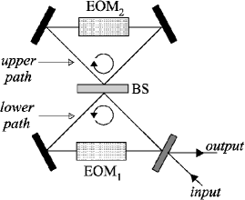
Figure 1: Optical cavity for the implementation of the OGB and the NLOGB. EOM₁ and EOM₂ are two electrooptic modulators which are tuned for incrementing (decreasing) the field frequency in $\Delta\omega$. BS is a beam–splitter, and the cavity is constituted by four mirrors, one of which is partially reflecting and serves as input/output port. For implementing the OGB, the upper and lower paths must be a linear optical medium, which must be replaced by a nonlinear optical medium (such as, e.g., an optical fiber) for implementing the NLOGB.

In this case, the QW occurs in the frequency distribution of the output field, with the intensity of each frequency component playing the role of the probability of finding the walker at a given position, i.e., $P_{m}^{u}(t)$ and $P_{m}^{d}(t)$ are spectral intensities in this classical–wave context, and not probabilities. In other words, after $m$ cavity roundtrips, the spectrum of the output field exhibits the probability distribution of the QW. This is one of the schemes proposed in Knight(b) for the optical (classical) implementation of the QW, where also the connection between the OGB of Ref. Bouwmeester and the QW is given, and we refer the reader to that paper for full details on this type of classical (optical) implementation of the QW. Let us emphasize that this scheme constitutes a realization of the optical Galton board.

What this classical implementation of the QW (and others Hillery ; Jeong ; Roldan ; Do05 ) suggests is that interference, and not entanglement, is the responsible of the QW characteristics. Entanglement would manifest in QWs in more than two dimensions, in the amount of classical resources needed for its implementation, as compared with a true quantum implementation, as already discussed in Knight(b) . This does not mean that there is nothing quantum in the QW: It is the different physical meaning of $P_{m}(t)$ (in a true quantum system, the probability distribution can be reconstructed only after a large enough number of measurements, while in the classical simulation the analog of the probability distribution corresponds to the field spectrum and can be seen completely at each walk step). The effect of decoherence could be different in classical and quantum implementations Kendon . But, at least in the QW on the line, the quantum nature seems not to manifest, as it can be successfully simulated by classical means. See Kendon05 for a discussion on this topic.

III Introducing the nonlinear optical Galton board.

The optical cavity scheme of Fig. 1 serves us to introduce the nonlinear optical Galton board (NLOGB). It suffices to assume that light acquires some intensity-dependent phase while traveling through the upper and lower paths, i.e., that these paths are not made by a linear medium (vacuum), but with a nonlinear medium (e.g. a Kerr medium, like an optical fiber or similar). This is very easily taken into account with the QW formalism introduced in the previous section that we will continue to use here: We only need to introduce one more operator describing the acquisition of the intensity-dependent (nonlinear) phase due to propagation in the Kerr medium, i.e., we have to generalize the unitary operator defined above in the following way:

$$\hat{U}(t)=\hat{U}_{d}\hat{U}_{c}\hat{U}_{nl}(t-1),$$ (4)

$$\hat{U}_{nl}(t)=\underset{c=u,d}{\sum}\underset{m}{\sum}e^{iF_{c}\left(m,t\right)}\left|c,m\right\rangle\left\langle c,m\right|,$$ (5)

where $F_{c}\left(m,t\right)$ $\left(c=u,d\right)$ is an arbitrary function of the probabilities (or intensities, in a classical context) $P_{m}^{u}(t)$ and $P_{m}^{d}(t)$ nota . Notice that the role of $\hat{U}_{nl}(t)$ is to add a nonlinear (probability dependent) phase to each of the spinor components. With the above formulation, the standard QW is obviously recovered when $F_{u}=F_{d}=0$, and the generalized QWs of Romanelli and Buerschaper ; Wojcik are recovered when $F_{u}=F_{d}=m^{2}\phi_{0}$ and $F_{u}=F_{d}=m\phi_{0}$, respectively, with $\phi_{0}$ a constant phase. We see that a physical system like the one represented in Fig. 1 allows to implement a number of interesting generalizations of the QW in a relatively simple way. Let us emphasize that the OGB of Bouwmeester et al. Bouwmeester is very close to what we are commenting Knight(b) .

In this article we shall consider one of the simplest forms for (5) by choosing $F_{c}\left(m,t\right)=2\pi\alpha\left|c_{m,t}\right|^{2}$ ($c=u,d$), i.e., we assume that the nonlinear phase gained between two QW steps is due to a Kerr-type nonlinearity that acts separately on the two coin states ($u$ and $d$) and has a strength $\alpha$. The recursive evolution equations for the probability amplitudes can be easily derived from $\left|\psi(t+1)\right\rangle=\hat{U}\left(t+1\right)\left|\psi(t)\right\rangle$, yielding

$$u_{m,t+1} =\frac{1}{\sqrt{2}}u_{m-1,t}e^{i2\pi\alpha\left|u_{m-1,t}\right|^{2}}$$ (6)

$$+\frac{1}{\sqrt{2}}d_{m-1,t}e^{i2\pi\alpha\left|d_{m-1,t}\right|^{2}},$$

$$d_{m,t+1} =\frac{1}{\sqrt{2}}u_{m+1,t}e^{i2\pi\alpha\left|u_{m+1,t}\right|^{2}}\text{ }$$ (7)

$$-\frac{1}{\sqrt{2}}d_{m+1,t}e^{i2\pi\alpha\left|d_{m+1,t}\right|^{2}}.$$

As we show below, the nonlinearity just introduced deeply modifies the behavior of the probability distribution $P_{m}(t)$. For this purpose, we perform a numerical study of Eqs. (6,7) for different values of $\alpha$. We shall consider $\alpha>0$ for definiteness, since from Eqs. (6,7) one easily sees that choosing a positive $\alpha$, say $\alpha=\alpha_{0}$, with some initial conditions $\left(u_{m,0};d_{m,0}\right)$ is equivalent to taking $\alpha=-\alpha_{0}$ and complex-conjugated initial conditions $\left(u_{m,0}^{\ast};d_{m,0}^{\ast}\right)$. Moreover, we shall adopt, unless otherwise specified, symmetrical initial conditions localized at the origin, i.e., $u_{m,0}=\delta_{m0}/\sqrt{2}$ and $d_{m,0}=i\delta_{m0}/\sqrt{2}$.

From a classical (wave) viewpoint, the above process is a nonlinear optical Galton Board (NLOGB) and can be implemented with the same device we have commented in the previous section, provided that the two optical beams propagate in a Kerr medium (e.g., an optical fiber), as this nonlinear propagation exactly corresponds to what $\hat{U}_{nl}$ represents. From a quantum viewpoint the implementation of $\hat{U}_{nl}$ is probably impossible because of the linearity of the Schrödinger equation. It is clear from now that the process we are proposing makes full sense only as a nonlinear OGB, and will find conceptual difficulties as a nonlinear QW.

In spite of the difficulties when speaking of a nonlinear QW, one should keep in mind that nonlinearities can be introduced in quantum systems through a clever use of measurement Knill ; Sanaka , what keeps open the possibility of implementing the proposed NLQW. Another, more realistic possibility concerns using systems described by nonlinear effective Hamiltonians, as Bose–Einstein condensation, where QWs could be implemented Chandrashekar , or superconducting devices, just to mention a couple of potential candidates. But these appear as remote possibilities, as compared with the immediacy of an optical implementation in an optical device similar to that already used by Bouwmeester et al. Bouwmeester .

IV Formation of soliton–like structures.

In Fig. 2 we represent the evolved probability distributions $P_{m}(t)$ for $\alpha=0$ (i.e., the standard QW) and $\alpha=0.4$. When $\alpha=0$, we observe the typical QW behavior reviews : $P_{m}(t)$ exhibits two peaks at the borders of the distribution, whose tails decay in the central zone, and whose maximum value monotonically decreases with time as the probability distribution broadens; and, most importantly, the width of $P_{m}(t)$ is proportional to $t$. This probability distribution can be expressed, in some limit Knight , as a combination of Airy functions propagating in opposite directions.

The shape of $P_{m}(t)$ for $\alpha=0.4$ is very different: Now the two peaks of $P_{m}(t)$ contain most of the total probability, around 30% each one in the case of Fig. 2, mostly distributed within a few lattice positions (see the inset in Fig. 2) . But the most striking characteristic of the probability peaks in this nonlinear case, is that their size and shape remain basically constant with time, except for small oscillations around a mean value.

We will characterize the probability peaks by their position and intensity (i.e., the total probability they contain). As for the position, given the small fluctuations on the shape of the peak, we use the "center of mass", defined as $m_{CM}\equiv\sum_{m}mP_{m}(t)$, with $m\in\left[m_{\max}+\Delta m,m_{\max}-\Delta m\right]$, $m_{\max}$ the position of the probability maximum and $\Delta m$ the width of the peak . Only small quantitative differences are found between the behavior of $m_{max}$ and that of $m_{CM}$.

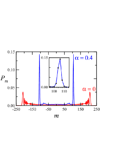
Figure 2: (Color online) Probability distribution curves of $P_{m}(t)$ for $t=300$, with the initial condition $u_{m,0}=\delta_{m0}/\sqrt{2}$ and $d_{m,0}=i\delta_{m0}/\sqrt{2}$, for $\alpha=0$ (standard QW) and $\alpha=0.4$. The inset is a magnification of the right–moving probability soliton. Notice that $P_{m}\left(t\right)$ is null for odd $m$ (as $t$ is even in this plot). We have represented only nonzero values and joined them for guiding the eye.

The most important feature of the probability peaks is that they are non-spreading pulses, i.e., they propagate without distortion . As these probability wave-packets do not spread in time, and present other particle–like features (see below) we can consider them as solitonic-like structures, and will simply refer to them as solitons.

Apparently, solitons do not require a minimum value of $\alpha$ to form: We have checked their existence for $\alpha\geq 0.01$, and the analysis of the data from different (non-zero) values of $\alpha$ does not suggest the existence of any threshold for the solitons formation. Nevertheless, the time needed for their formation (i.e., the transient until the intensity and shape of the probability structure is constant on the average) is larger for smaller $\alpha$. This is appreciated in Fig. 3 (a), where the intensity of a single soliton is represented as a function of time for different values of the nonlinearity parameter $\alpha$. Another important feature is that the width of the overall probability distribution $P_{m}(t)$ or, equivalently, the soliton velocity, decreases as $\alpha$ increases, as shown in Fig. 3 (b), where the position of the solitons is represented for different values of $\alpha$ (in the case $\alpha=0$, where solitons do not exist, we have represented the position of the center of mass of the maximum of $P_{m}\left(t\right)$ for the sake of comparison). Therefore, solitons form after some transient, and are slower and more intense for larger $\alpha$. This is the scenario we found for $\alpha\leq 0.474$.

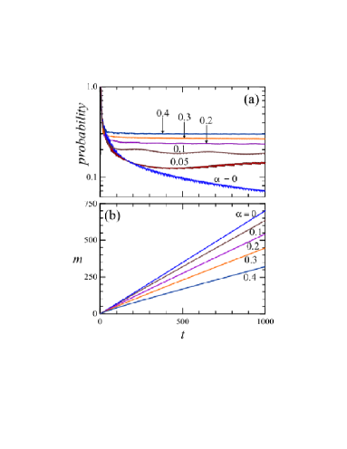
Figure 3: (Color online) (a) Intensity (total probability) of the right–moving soliton. (b) Temporal evolution of the center of mass, $m_{CM}$, of the right–moving soliton (the plot is symmetric for the left-moving soliton). The values of $\alpha$ are indicated in the plots. Initial conditions are as in Fig. 2.

In view of the phenomena described above, one might wonder whether the intrinsic quantum features of QWs are deteriorated or not, and if so, to what extent. One way to quantify the possible loss of the quantum benefits is by analyzing the time evolution of the standard quadratic deviation $\sigma=\sqrt{<m{{}^{2}}>-<m>{{}^{2}}}$ . As already discussed, the standard QW exhibits a characteristic $\sigma\propto t$. Given the transient which appears during the formation of the solitons, the question we ask ourselves is: does the quotient $\sigma/t$ go to a constant after the transient (i.e., for sufficiently large time), or will it decay slower?

As can be seen from Fig. 4, the first possibility is in fact realized: after the transient, the standard deviation approaches the typical QW time evolution. Therefore, the long-term QW behavior is not degraded by the formation and propagation of the solitons.

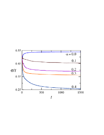
Figure 4: (Color online) Evolution of the ratio $\sigma/t$ for different values of $\alpha$.

V Dynamical phases.

We have been able to identify three different dynamical domains, or dynamical phases, in the behavior of solitons as a function of the value of $\alpha$: Phase I, for $\alpha<\alpha_{I}\simeq 0.474$; phase II, for $\alpha_{I}<\alpha<\alpha_{II}\simeq 0.6565$; and phase III, for $\alpha>\alpha_{II}$. Let us describe these phases separately.

In Phase I, the dynamics is very simple: Once solitons have formed, they exhibit the ballistic propagation already shown in Fig. 3(b). Differently, in Phase II the two solitons start moving in opposite directions, as in Phase I, but after some time their velocity decrease till the solitons reach a turning point and then move backwards and collide at some later instant $t_{col}$ at $m=0$. After the collision, the solitons continue moving apart indefinitely, as in phase I. An example of such behavior, for $\alpha=0.49$, is shown in Figure 5. Notice the appearance of small “communication packets” that are interchanged between the two solitons. Interestingly, the solitons intensity sharply decreases after the collision (for example, for $\alpha=0.49$ the intensity of one soliton falls from $0.3062$ before the collision, to $0.2426$ afterwards), i.e., the collision of the two solitons is an inelastic one. Another feature that can be observed from the simulations is that, as $\alpha$ is increased from below $\alpha_{I}$ (inside phase I), the intensity of the solitons increase up to a maximum value. It seems that the communication packets interchanged by the two solitons play the role of an attractive interaction, which is larger for larger intensities. This would explain the existence of the above-mentioned turning point appearing at some critical value $\alpha_{I}$. Inside phase II, the solitons experience an inelastic scattering and loose a fraction of their intensity, which would prevent from recollapse.

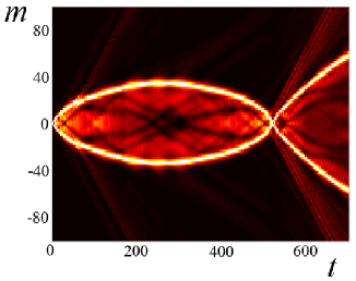
Figure 5: (Color online) Color density plot showing the evolution of $P_{m}(t)$ as a function of $t$ (horizontal axis) for $\alpha=0.49$. The vertical axis corresponds to the position on the lattice. Brighter regions indicate a higher probability. The two solitons are clearly visualized as intense strips.

The method we used to determine this critical value, however, makes use of the fact that the collision instant $t_{col}$ decreases with $\alpha$. Indeed, the function $t_{col}(\alpha)$ can be well reproduced numerically by a simple hyperbola $1/t_{col}=a/\alpha+b$ (where the values of $a$ and $b$ are obtained by a numerical fit, with a coefficient of determination $r^{2}=0.99516$, giving $a=-0.0297\pm 0.0003$ and $b=0.0627\pm 0.0006$). This numerically-obtained law allows to fix the frontier between phases I and II by the $\alpha$ value for which $t_{col}$ diverges (we obtained $\alpha_{I}=0.474\pm 0.007$).

As we made for phase I, it is worth investigating how the standard deviation evolves at long times, in order to quantify a possible departure from the characteristic quantum spreading. As before, we plot in Fig. 6 the quotient $\sigma/t$ as a function of time for values of $\alpha$ corresponding to the second phase. Now the transient shows more complicated features, due to the recollapse of the two solitons (which manifests as the minimum appearing in both curves). However, as the solitons separate after the collision, the typical $\sigma\propto t$ behavior shows up.

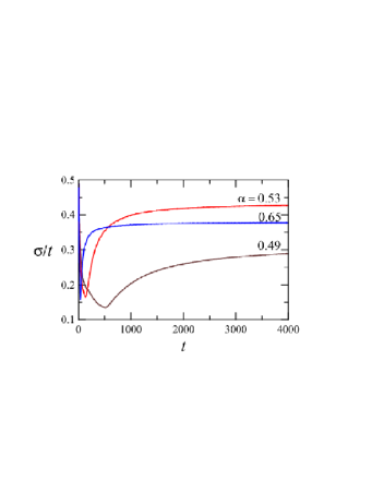
Figure 6: (Color online) Same as Fig. 4, for values of $\alpha$ corresponding to phase II.

Phase III, $\alpha>\alpha_{II}$, differs from phase II in that, after the collision, the two emerging solitons do not necessarily collide or separate from each other. In fact, if $\alpha$ is increased beyond $\alpha_{II}$, the situation becomes quite complicated, as the evolution of the solitons becomes extremely sensitive to small variations in $\alpha$. In this sense, we can say that phase III is a chaotic phase: For some values of $\alpha$, the solitons become trapped and oscillate around the origin; with a slightly different value for $\alpha$, however, the solitons eventually escape; and there are other $\alpha$ values for which localization is found, which is characterized by an asymptotic setup of both solitonic structures at an equilibrium point. Interestingly, the latter possibility can occur at very distant site positions for slightly different values of $\alpha$: For example, the right-moving soliton position oscillates between $m=5$ and $m=9$ for $\alpha=0.6665$; it remains static at position $m=162$ for $\alpha=0.6669$; and again oscillates, around $m=7$, for $\alpha=0.6673$. In Fig. 7 we show an example of the type of dynamics one encounters in phase III for the two values of $\alpha$ indicated in the figure caption.

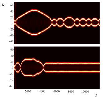
Figure 7: (Color online) Same as Fig. 5, but for $\alpha=$$0.6565$ (top) and $\alpha=0.658197$ (bottom).

The results we have just described correspond to a particular choice of the QW initial conditions, which guarantees the symmetry of the probability distribution with respect to the starting position. In order to see how critical is the role of the initial condition, we have carried out numerical simulations for different sets of initial conditions, and have found that the dynamics is also very sensitive to this choice. Fig. 8 gives an idea of how different things can be: we represent the evolution of the probability distribution for $u_{m,0}=\delta_{m0},d_{m,0}=0$ and $\alpha=0.2$ (top) or $\alpha=0.6$ (bottom). For this initial condition, the probability distribution is no longer symmetric (even in the standard QW), and this fact strongly affects the formation and dynamics of solitons. We are not going to enter into an exhaustive description here; it will suffice to say that, in this case, there are also several dynamic phases: For small $\alpha$, a single soliton forms, carrying close to 60% of the probability, that moves like in Fig. 7 (top) (most of the rest of the probability is contained in small dispersive pulses that can be appreciated in the figure); for large $\alpha$ several solitons, with different intensities, can form, and localization phenomena similar to what we have described above can occur too, see Fig. 8 (bottom).

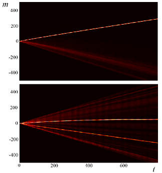
Figure 8: (Color online) Same as Fig. 5, but for $\alpha=0.2$ (top) and $\alpha=0.6$ bottom. The initial conditions are $u_{m,0}=\delta_{m0}$ and $d_{m,0}=0$. For $\alpha=0.2$ a single soliton is formed that carries 57% of the probability. For $\alpha=0.6$ this soliton has now a smaller intensity (32% of the probability) and becomes localized near $m=0$, while a second soliton (20% of the probability) is formed.

VI Conclusions.

We have introduced a simple variation of the Optical Galton Board (which can be understood as a classical implementation of the discrete coined QW), based on the assumption that light propagates through a nonlinear (Kerr-type) medium inside the optical cavity or, using the algebraic language of QW, based on the acquisition of non-linear -probability dependent- phases by the state during the walk.

The most striking feature that the nonlinearity introduces, is the formation of soliton-like structures, which carry a constant fraction of the total intensity (probability) distribution within a non-dispersive pulse. We have characterized the dynamics of these solitons showing the existence of complex dynamics (from ballistic motion to dynamical localization) that is very sensitive to the initial conditions. An important feature we found is that, in spite of the complicated behavior during the transient and possible recollapse of the solitons, the long term evolution still shows the characteristic QW feature in the cases when the solitons go away, in the sense that the standard deviation becomes $\sigma\propto t$.

It would be of greatest interest to have at hand an analytical description of the solitons motion and interaction, specially during the formation transient and recollapse (when present), as done (approximately) in [10]. The additional complication due to non-linearities, however, makes this task cumbersome and lies beyond the scope of this paper.

The described phenomena are, to the best of our knowledge, new in the field of quantum walks. The exciting features found here deserve, we believe, further research.

Acknowledgments

We gratefully acknowledge fruitful discussions with G.J. de Valcárcel. This work has been supported by the Spanish Ministerio de Educación y Ciencia and the European Union FEDER through Projects FIS2005-07931-C03-01, AYA2004-08067-C01, FPA2005-00711 and by Generalitat Valenciana (grant GV05/264).

References

- (1) R. Motwani and P. Raghavan, Randomized Algorithms (Cambridge University Press, 1995).
- (2) Y. Aharonov, L. Davidovich, and N. Zagury, Phys. Rev. A 48, 1687 (1993).
- (3) D. Meyer, J. Stat. Phys. 85, 551 (1996).
- (4) J. Watrous, Proc. 33rd Symposium on the Theory of Computing (ACM Press, New York, 2001), p.60.
- (5) E. Farhi and S. Gutman, Phys. Rev. A 58, 915 (1998); A.M. Childs and J. Goldstone, Phys. Rev. A 70, 042312 (2004).
- (6) For reviews, see J. Kempe, Contemp. Phys. 44, 307 (2003); A. Ambainis, Int. J. Quantum Inform. 1, 507 (2003); V. Kendon, Phil. Trans. R. Soc. A 364, 3407 (2006).
- (7) V. Kendon, quant-ph/0606016
- (8) D. Bouwmeester, I. Marzoli, G.P. Karman, W. Schleich, and J.P. Woerdman, Phys. Rev. A 61, 013410 (2000).
- (9) B.C. Sanders, S.D. Bartlett, B. Tregenna, and P.L. Knight, Phys. Rev. A 67, 042305 (2003).
- (10) P.L. Knight, E. Roldán, and J.E. Sipe, Opt. Commun. 227, 147 (2003); erratum 232, 443 (2004).
- (11) P.L. Knight, E. Roldán, and J.E. Sipe, Phys. Rev. A 68, 020301(R) (2003).
- (12) A. Wojcik, T. Lukzak, P. Kurzynski, A. Grudka, and M. Bednarska, Phys. Rev. Lett. 93, 180601 (2004).
- (13) A. Romanelli, A. Auyuanet, R. Siri, G. Abal and R. Donangelo, Physica A 352, 409 (2005).
- (14) O. Buerschaper and K. Burnett, quant-ph/0406039.
- (15) M.C. Bañuls, C. Navarrete, A. Pérez, E. Roldán, and J.C. Soriano, Phys. Rev. A 73, 062304 (2006).
- (16) I. Carneiro et al., New Journal of Physics 7, 156 (2005).
- (17) R.J.C. Spreeuw, Phys. Rev. A 63, 062302 (2001).
- (18) M. Hillery, J. Bergou, and E. Feldman, Phys. Rev. A 68, 032314 (2003).
- (19) H. Jeong, M. Paternostro, and M.S. Kim, Phys. Rev. A 69 012310 (2004).
- (20) E. Roldán and J. C. Soriano, J. Mod. Opt. 52, 2649 (2005).
- (21) B. Do, M.L. Stohler, S. Balasubramanian, D.S. Elliot, Ch. Eash, E. Fischbach, M.A. Fischbach, A. Mills, and B. Zwickl, J. Opt. Soc. Am. 22, 499 (2005).
- (22) V. Kendon and B. Tregenna, Phys. Rev. A 71, 022307 (2005).
- (23) We must emphasize that and are probabilities in a true quantum system, but in a classical system they are intensities, see e.g. Knight .
- (24) E. Knill, R. Laflamme, and G.J. Milburn, Nature 409, 46 (2001).
- (25) K. Sanaka, K.J. Resch, and A. Zeilinger, Phys. Rev. Lett. 96, 083601 (2006).
- (26) C.M. Chandrashekar, Phys. Rev. A 74, 032307 (2006).