Aspects of quantum coherence in the optical Bloch equations

Abstract

Aspects of coherence and decoherence are analyzed within the optical Bloch equations. By rewriting the analytic solution in an alternate form, we are able to emphasize a number of unusual features: (a) despite the Markovian nature of the bath, coherence at long times can be retained; (b) the long–time asymptotic degree of coherence in the system is intertwined with the asymptotic difference in level populations; (c) the traditional population–relaxation and decoherence times, $T_{1}$ and $T_{2}$, lose their meaning when the system is in the presence of an external field, and are replaced by more general overall timescales; (d) increasing the field strength, quantified by the Rabi frequency, $\Omega$, increases the rate of decoherence rather than reducing it, as one might expect; and (e) maximum asymptotic coherence is reached when the system parameters satisfy $\Omega^{2}=1/(T_{1}T_{2})$.

I Introduction

A quantum system whose dynamics is of interest is often part of, or coupled to, a second system whose dynamics is irrelevant. Examples include the internal quantum dynamics of a molecule in solution, a qubit imbedded in a solid, the translational motion of a single particle in a gas, the dynamics of one part of a molecule, etc. The overall dynamics of the total system is given by the Hamiltonian

$$\hat{H}=\hat{H}_{S}+\hat{H}_{B}+\hat{V}_{SB},$$ (1)

where $\hat{H}_{S}$ and $\hat{H}_{B}$ describe, respectively, the free evolution of the system of interest (that we henceforth refer to as the “system”) and the extraneous degrees of freedom (termed the “bath”), and $\hat{V}_{SB}$ accounts for their interaction. Ideally, the system dynamics is obtained by solving the Schrödinger equation for the full Hamiltonian, $\hat{H}$, and then averaging over the bath degrees of freedom. However, more often than not, this route is intractable. Hence, it is common to replace the full dynamics associated with Eq. (1) by an approximate master equation percival ; breuer ; accardi for the system density matrix, $\hat{\rho}_{S}\equiv{\rm Tr}_{B}\left[\ \!\hat{\rho}\ \!\right]$. This type of equation provides a description of the two effects induced by the bath on the system: population changes and coherence loss.

Recently, the degree of quantum coherence of a system has become increasingly important. For example, both the coherent control of molecular processes riceb ; brumerb and quantum manipulations in quantum computing, quantum information and quantum cryptography unruh ; ekert ; viola ; qirefs , rely upon the ability to keep the coherence of a system as well as to counter the decohering effects induced by the environment. One long–standing approach to reintroduce coherence in a system that is interacting with a bath is to irradiate the system with a coherent electromagnetic field.

In this paper we provide new insights into the coherence and decoherence in a paradigmatic two–level system interacting with a decohering environment and a resonant continuous–wave (CW) electromagnetic field. The model that we focus upon is the standard Bloch equation bloch wherein the bath is Markovian, i.e., the coherence that is transferred to the bath is lost from the system forever. Using an alternate to the standard solution to this analytic problem torrey ; allen , we show that useful new insights emerge into the way in which the thermal bath and the external electromagnetic field interact to produce and sustain coherence in the system. Specifically, we emphasize that (a) despite the Markovian nature of the bath, coherence at long times can be retained; (b) the long–time asymptotic degree of coherence in the system is intertwined with the asymptotic difference in level populations; (c) the traditional population–relaxation and decoherence times, $T_{1}$ and $T_{2}$, lose their meaning when the system is in the presence of an external field, and are replaced by a more general overall timescale; (d) increasing the field strength, quantified by the Rabi frequency, $\Omega$, increases the rate of decoherence rather than reducing it, as one might expect; and (e) maximum asymptotic coherence is reached when the system parameters satisfy $\Omega^{2}=1/(T_{1}T_{2})$.

The organization of this work is as follows. A brief description of the two–level system is presented in Sec. II. The asymptotic and time–dependent solutions to this model are discussed in Sec. III. Finally, the main conclusions derived from this work are summarized in Sec. IV.

II The two level system

The dynamical evolution of a two–level system influenced by a thermal bath can be modelled by means of the master equation

$$\frac{d\hat{\rho}_{S}}{dt}=-\frac{i}{\hbar}\left[\hat{H}^{\prime}(t),\hat{\rho}_{S}\right]-\mathcal{R}\ \!\hat{\rho}_{S},$$ (2)

where $\hat{H}^{\prime}(t)=\hat{H}_{S}+\hat{H}_{\rm int}(t)$, and $\mathcal{R}$ is a superoperator describing the evolution of the bath and its effects on the system (i.e., $\hat{H}_{B}+\hat{H}_{SB}$). The evolution of the isolated (free) two–level system is determined by the Hamiltonian

$$\hat{H}_{S}=\sum_{i=1,2}E_{i}|i\rangle\langle i|,$$

and

$$\hat{H}_{\rm int}=-E(t)\sum_{\begin{subarray}{c}i,j=1,2\\ i\neq j\end{subarray}}\hat{\bf d}|i\rangle\langle j|,$$

which accounts for the atom–field interaction within the dipole approximation, with $E(t)=\mathcal{E}\cos(\omega t+\varphi)$ and $\mathcal{E}$ being the strength of the electromagnetic field.

The simplest model for dynamics of this type is the Markovian Bloch equation,

$$\frac{d\rho_{i,j}}{dt}=-\frac{i}{\hbar}\left[\hat{H}^{\prime}(t),\hat{\rho}\right]_{i,j}-\frac{1}{T_{i,j}}\ \!\rho_{i,j}.$$ (3)

where $\mathcal{R}$ is written in terms of the phenomenological relaxation times: $T_{1}=T_{i,i}$ and $T_{2}=T_{i,j}$ ($i\neq j$). In the absence of the electromagnetic field, $T_{1}$ provides the timescale for changes in the system (eigenstate) populations, $\rho_{i,i}(t)$, with a rate given by $\Gamma_{1}=1/T_{1}$. Due to system–bath elastic collisions, there are random changes in the system phases that affect the off–diagonal terms $\rho_{i,j}(t)$ ($i\neq j$) and subsequently lead to system decoherence at a rate $\Gamma_{2}=1/T_{2}$.

In the most general approach the values of $T_{1}$ and $T_{2}$ are not constrained. For example, Skinner and coworkers have shown skinner1 ; skinner2 , using a non–Markovian model of a two–level system linearly and off–diagonally coupled to a harmonic quantum–mechanical bath, that $T_{2}$ can actually be greater than $2T_{1}$, with $T_{2}=2T_{1}$ in the weak coupling limit. In the case of the standard Bloch equation bloch , however, one has

$$2T_{1}\geq T_{2}$$ (4)

in order to ensure that the reduced dynamics for the system always leads to completely positive maps of the density matrix Daffer , i.e., that ${\rm Tr}\left[\ \!\hat{\rho}_{S}^{2}\ \!\right]\leq 1$ at any time. Thus, although the Bloch equation is mathematically well–defined for any values of $T_{1}$ and $T_{2}$, they lose their physical meaning when Eq. (4) is not satisfied. Here, the condition (4) is retained throughout the study.

Equation (3) can be solved within the rotating–wave approximation allen2 by introducing the following change of variables note1 :

$$R_{1} = 2\ \!{\rm Im}\left[\ \!\rho_{12}\ \!\right]=-i(\rho_{12}-\rho_{21}),$$

$$R_{2} = 2\ \!{\rm Re}\left[\ \!\rho_{12}\ \!\right]=\rho_{12}+\rho_{21},$$ (5)

$$R_{3} = \rho_{11}-\rho_{22}.$$

Here, $R_{3}$ is the difference in population between the two levels, and $R_{1}$ and $R_{2}$ are the imaginary and real components of the off–diagonal density matrix elements. With these new variables, Eq. (2) can then be rewritten note2 in the standard form of the optical Bloch equations for a two–level system as

$$\frac{dR_{1}}{dt} = -\Gamma_{2}R_{1}+\Delta R_{2}+\Omega R_{3},$$ (6a)

$$\frac{dR_{2}}{dt} = -\Delta R_{1}-\Gamma_{2}R_{2},$$ (6b)

$$\frac{dR_{3}}{dt} = -\Omega R_{1}-\Gamma_{1}(R_{3}-\tilde{R}_{3}),$$ (6c)

where $\Omega=2d_{12}\mathcal{E}/\hbar$ (with $d_{12}=\langle 1|\hat{\bf d}|2\rangle$) is the Rabi frequency with which the system oscillates between the two levels in the absence of a bath, and $\Delta=(E_{2}-E_{1})/\hbar-\omega$ is the detuning of the laser frequency $\omega$ from the $|E_{1}\rangle\to|E_{2}\rangle$ transition.

The quantity $\tilde{R}_{3}$ in Eq. (6c) is the thermal equilibrium population difference to which $R_{3}$ asymptotically relaxes in the absence of the external field, and is defined as

$$\tilde{R}_{3}=\frac{1-e^{-\hbar\omega_{2,1}/k_{B}T}}{1+e^{-\hbar\omega_{2,1}/k_{B}T}},$$ (7)

with $\omega_{2,1}=(E_{2}-E_{1})/\hbar$. $\tilde{R}_{3}$ indicates the degree of mixedness of the reduced density matrix at temperature $T$ and in the absence of the external field ($\Omega=0$). Two limits are therefore evident: (a) $\tilde{R}_{3}\to 1$ if $T\to 0$, and (b) $\tilde{R}_{3}\to 0$ if $T\to\infty$.

III Results and Discussion

III.1 Asymptotic Coherence

Our interest focuses on the nature of the system coherence and its dependence on the system and field parameters. Two quantities serve as useful measures of coherence: the purity, $\chi$, and the interference contribution, $\zeta$. The purity is given by

$$\chi={\rm Tr}\left[\ \!\hat{\rho}_{S}^{2}\ \!\right] = \rho_{11}^{2}+\rho_{22}^{2}+2|\rho_{12}|^{2}$$ (8)

$$= \frac{1}{2}+\frac{1}{2}\left(R_{1}^{2}+R_{2}^{2}+R_{3}^{2}\right),$$

and depends on both level populations and interference. By contrast, the interference contribution, which we define as

$$\zeta=|\rho_{12}|^{2}=\frac{1}{4}\left(R_{1}^{2}+R_{2}^{2}\right),$$ (9)

describes the coherence in the energy basis. Hence, though far from an ideal measure of decoherence, $\chi$ is particularly useful due to its basis–independence.

At long times, when the system reaches the equilibrium, all time derivatives in Eqs. (6) are zero, and the (asymptotic) value of the $R_{i}$ becomes, for the on-resonance case ($\Delta=0$) emphasized below,

$$R_{1}^{\rm eq} = -\frac{\Gamma_{1}\Omega}{\Gamma_{1}\Gamma_{2}+\Omega^{2}}\ \!\tilde{R}_{3},$$

$$R_{2}^{\rm eq} = 0,$$

$$R_{3}^{\rm eq} = \frac{\Gamma_{1}\Gamma_{2}}{\Gamma_{1}\Gamma_{2}+\Omega^{2}}\ \!\tilde{R}_{3}.$$

Consequently, inverting Eqs. (5) gives the reduced density matrix elements note3 :

$$\rho_{12}^{\rm eq} = \left(\rho_{21}^{\rm eq}\right)^{*}=\frac{1}{2}\bigg{[}\frac{T_{2}\Omega}{1+T_{1}T_{2}\Omega^{2}}\bigg{]}e^{i(2\varphi-\pi/2)}\tilde{R}_{3},$$ (10a)

$$\rho_{11}^{\rm eq} = \frac{1}{2}\bigg{[}1+\frac{\tilde{R}_{3}}{1+T_{1}T_{2}\Omega^{2}}\bigg{]},$$ (10b)

$$\rho_{22}^{\rm eq} = \frac{1}{2}\bigg{[}1-\frac{\tilde{R}_{3}}{1+T_{1}T_{2}\Omega^{2}}\bigg{]},$$ (10c)

where it is apparent that $\rho_{11}^{\rm eq}\geq\rho_{22}^{\rm eq}$. Observe that

$$\rho_{12}^{\rm eq}=-\frac{1}{2}\ \!T_{2}\Omega\ \!e^{i(2\varphi+\pi/2)}\left[\rho_{11}^{\rm eq}-\rho_{22}^{\rm eq}\right],$$ (11)

giving a relationship between the coherence elements of the reduced density matrix and the population difference.

Numerous features regarding the coherence at long times are evident from Eqs. (10). Obviously, the coherence is totally lost ($\zeta=0$) in the absence of the field ($\Omega=0$). Most significantly, as emphasized further below, the asymptotic extent of the coherence (as manifest in the value of $\rho_{12}^{\rm eq}$) is directly proportional to $\tilde{R}_{3}$, the difference between the final populations of each state. Thus, for example, if the temperature is high, $\tilde{R}_{3}=0$ and $\zeta=0$ regardless of the initial conditions. Similarly, at lower temperatures, and also regardless of initial conditions, the asymptotic value of $\zeta$ can be nonzero, and the system can have therefore gained coherence due to the combined influence of the non–zero asymptotic population difference (related to the nature of the environment) and the field.

Studies that focus solely on decoherence viola often neglect population–relaxation processes by setting $T_{1}=\infty$. In this case [from Eq. (10a)], all coherence is lost at equilibrium, with $\rho_{12}^{\rm eq}=0$. Hence, long–time coherences that can exist in the case of finite $T_{1}$ are missed. This reliance of long–time coherence emphasizes the significant interplay between the long–time population difference, $R_{3}^{\rm eq}$, the time that it takes to reach that limit (as manifest in $T_{1}$ timescales), and the long–time coherence, $\rho_{12}^{\rm eq}$.

Interestingly, coherence loss also occurs with large $\Omega$, as is evident in Eq. (10a). That is, $|\rho_{12}^{\rm eq}|$ is an increasing function of $\Omega$ until $\Omega^{2}=1/(T_{1}T_{2})$, at which point $|\rho_{12}^{\rm eq}|=\sqrt{T_{2}/T_{1}}\ \!\tilde{R}_{3}/4$. Increasing $\Omega$ beyond this value causes a decrease in the asymptotic coherence. Note that in the particular case where $T_{1}$ is assumed very large, the asymptotic coherence is a decreasing function of $\Omega$ for almost all $\Omega$ values.

III.2 Time Evolution

The analytic solution to Eqs. (6) for the time evolution of the $R_{i}$ is known torrey . Here we rewrite it in a somewhat more enlightening form.

Consider the case of on–resonance excitation ($\Delta=0$). Laplace transforming Eq. (6c), and defining the transforms with over–bars, leads to the following linear system:

$$(s+\Gamma_{2})\bar{R}_{1}+\Omega\bar{R}_{3} = R_{1}^{(0)},$$ (12a)

$$(s+\Gamma_{2})\bar{R}_{2} = R_{2}^{(0)},$$ (12b)

$$(s+\Gamma_{1})\bar{R}_{3}-\Omega\bar{R}_{1} = R_{3}^{(0)}+\Gamma_{1}\tilde{R}_{3}/s,$$ (12c)

where the $R_{i}^{(0)}$ are the initial conditions for each of the variables.

As seen from Eq. (12b), the time–dependence of $R_{2}$,

$$R_{2}(t)=R_{2}^{(0)}e^{-\Gamma_{2}t},$$ (13)

is readily obtained, since this variable is uncoupled from the other two. Therefore, for fixed $T_{2}$ and $T_{1}>T_{2}$, the dynamics is described by $R_{1}$ and $R_{3}$ beyond times on the order of $T_{2}$.

To obtain $R_{1}$ and $R_{3}$, the value of $\bar{R}_{1}$ resulting from Eq. (12c) is substituted into (12a), giving

$$\left[(s+\Gamma_{1})(s+\Gamma_{2})+\Omega^{2}\right]\bar{R}_{3}=\Omega R_{1}^{(0)}+(s+\Gamma_{2})R_{3}^{(0)}+\frac{(s+\Gamma_{2})\Gamma_{1}}{s}\ \!\tilde{R}_{3},$$ (14)

where the roots of the factor multiplying $\bar{R}_{3}$ are $s_{\pm}=-\alpha\pm\beta$, with

$$\alpha=\frac{\Gamma_{1}+\Gamma_{2}}{2},\ \ \ \beta=\frac{\sqrt{(\Gamma_{2}-\Gamma_{1})^{2}-4\Omega^{2}}}{2}.$$

Depending on the magnitude of the discriminant of $\beta$, three cases result. If $|\Gamma_{2}-\Gamma_{1}|\neq 2\Omega$, then

$$\bar{R}_{3}=\frac{D_{3}}{s}+\frac{B_{3}}{s-s_{-}}+\frac{C_{3}}{s-s_{+}},$$ (15)

with

$$D_{3} = \frac{\Gamma_{1}\Gamma_{2}}{s_{-}s_{+}}\tilde{R}_{3}=\frac{\Gamma_{1}\Gamma_{2}}{\Gamma_{1}\Gamma_{2}+\Omega^{2}}\tilde{R}_{3},$$ (16a)

$$B_{3} = \frac{s_{-}^{2}R_{3}^{(0)}+s_{-}\Lambda+\Gamma_{1}\Gamma_{2}\tilde{R}_{3}}{s_{-}(s_{-}-s_{+})},$$ (16b)

$$C_{3} = \frac{s_{+}^{2}R_{3}^{(0)}+s_{+}\Lambda+\Gamma_{1}\Gamma_{2}\tilde{R}_{3}}{s_{+}(s_{+}-s_{-})},$$ (16c)

where $\Lambda\equiv\Omega R_{1}^{(0)}+\Gamma_{2}R_{3}^{(0)}+\Gamma_{1}\tilde{R}_{3}$. The inverse Laplace transform of Eq. (15) leads to

$$R_{3}(t)=D_{3}+\left(B_{3}e^{-\beta t}+C_{3}e^{\beta t}\right)e^{-\alpha t}.$$ (17)

Now, introducing Eq. (17) into Eq. (12a), we obtain for the imaginary part of the coherence

$$R_{1}(t)=D_{1}+\left(B_{1}e^{-\beta t}+C_{1}e^{\beta t}\right)e^{-\alpha t},$$ (18)

with

$$D_{1} = -\frac{\Gamma_{1}\Omega}{\Gamma_{1}\Gamma_{2}+\Omega^{2}}\tilde{R}_{3},$$

$$B_{1} = \frac{(s_{-}+\Gamma_{1})}{\Omega}\ \!B_{3},$$

$$C_{1} = \frac{(s_{+}+\Gamma_{1})}{\Omega}\ \!C_{3}.$$

Therefore, for $|\Gamma_{2}-\Gamma_{1}|\neq 2\Omega$, both $R_{1}$ and $R_{2}$ decay exponentially. However, for $|\Gamma_{2}-\Gamma_{1}|<2\Omega$, $\beta$ is imaginary, and $R_{1}$ and $R_{3}$ oscillate as they decay. Below, the time–dependent factors depending on $\beta$ and that are responsible for the fine structure of the decays will be labelled $F_{i}$.

Specific results for the case of “critical damping”, $|\Gamma_{2}-\Gamma_{1}|=2\Omega$, can be obtained by considering the limit of the previous expressions when $\beta\to 0$ (for which $s_{\pm}=s_{0}=-\alpha$). In this case both $R_{1}$ and $R_{3}$ exponentially decay with rate $\alpha$, although the $F_{i}$ are linear functions of time.

These results [Eqs. (17) and (18)] allow direct consideration of the rates of falloff observed for the populations and coherences in the presence of a non–zero field. Specifically, if the field is strong ($2\Omega\geq|\Gamma_{2}-\Gamma_{1}|$) both the populations and the coherences decay with an overall rate $\alpha\leq\Gamma_{2}$ whenever $T_{1}\geq T_{2}$, albeit with superposed oscillations. Thus, in principle, there is no distinction between the falloff rates of the diagonal and off–diagonal elements of the density matrix. This is also evident in $\chi$, where the long–time decay goes as $2\alpha=\Gamma_{1}+\Gamma_{2}$, and it is not possible to clearly distinguish between two different timescales in its evolution. Nonetheless, since the $B_{i}$ and $C_{i}$ depend on $\Omega$, the amplitude of the $F_{i}$ can be greater than unity, and therefore may lead to slower $\chi$ decay rates than $2\alpha$ at early times despite being multiplied by the exponential. In the limit of $\Omega\to\infty$, the $F_{i}$ become highly oscillatory functions of time with decreasing amplitude about $F_{i}=1$, and the decay rate exactly corresponds to $2\alpha$. This can be easily seen by substituting Eqs. (13), (17), and (18) into Eq. (8). For example, for an initial state comprised of population in the state $|1\rangle$ (i.e., $R_{1}^{(0)}=R_{2}^{(0)}=0$, $R_{3}^{(0)}=1$), one obtains

$$\chi=\frac{1}{2}+\frac{1}{2}\left[1+2\left(\frac{\Gamma_{2}-\Gamma_{1}}{2\beta}\right)^{2}\sin^{2}\beta t+\left(\frac{\Gamma_{2}-\Gamma_{1}}{2\beta}\right)\sin 2\beta t\right]e^{-2\alpha t},$$ (19)

which effectively approaches

$$\chi=\frac{1}{2}+\frac{1}{2}\ \!e^{-2\alpha t},$$ (20)

when $\Omega\to\infty$ (and therefore $\beta\to\Omega$).

If the field is weaker ($2\Omega<|\Gamma_{2}-\Gamma_{1}|$) there are two system decay rates for $R_{1}$ and $R_{3}$, $\alpha\pm\beta$, with the smaller of the two dominating at longer time. In the parameter region where $2\Omega<|\Gamma_{2}-\Gamma_{1}|$, the decay rate increases with increasing $\Omega$, evidently reaching its maximum, in this region, at critical damping. However, numerical evidence reported below shows that the decay rate continues its increase with increasing $\Omega$ in the stronger field region, where $2\Omega\geq|\Gamma_{2}-\Gamma_{1}|$. Note that only in the limit of very small $\Omega$ does the standard field–free interpretation ($R_{1}$ and $R_{2}$ decaying with rate $\Gamma_{2}$, and $R_{3}$ with rate $\Gamma_{1}$) apply, since both $B_{3}$ and $C_{1}$ approach zero in this limit.

III.2.1 $T=\infty$

Consider first the case where $T=\infty$. Here, the field is unable to beat out, at long time, the thermalizing effects of the bath, thus leading to zero asymptotic coherence. This happens even if the field is CW and is on for all time. The coherence dynamics on the way to the asymptotic result is of interest. As an indication of the non–intuitive nature of the associated relaxation timescales, consider the results for $\zeta$ and $\chi$, shown in Figs. 1(a) and (b). A grey scale is used to indicate the magnitude of $\zeta$ and $\chi$ as a function of $t$ and $\Omega$ for an initial state comprised of population in $|1\rangle$. A number of interesting features can be observed. First, as noted above, the decay rate increases with increasing $\Omega$, even beyond the case of $2\Omega=|\Gamma_{2}-\Gamma_{1}|\simeq 1.33$. Further, the onset of oscillatory falloff above this value is clearly visible. The (overall) falloff timescale, given by $(2\alpha)^{-1}$, is in this case $\approx 0.375$, making evident the inseparability of the meaning of $T_{1}$ and $T_{2}$ (i.e., one cannot observe two clearly separated decay timescales in $\chi$).

The alternative perspective in Figs. 2(a) and (b), where $\zeta$ and $\chi$ are shown as a function of $\log_{10}T_{2}$ and time for fixed $T_{1}=2.5$ and $\Omega=1$ is also enlightening. In this case, the rate of decay of $\zeta$ and $\chi$ are seen to fall off increasingly rapidly as $T_{2}$ becomes larger, until $|\Gamma_{2}-\Gamma_{1}|=2\Omega$, (here corresponding to log${}_{10}T_{2}=-0.2$). At this point, with increasing $T_{2}$, the rate of falloff slows down and oscillates (these oscillations are better appreciated in the case of $\zeta$). The effect becomes increasingly exaggerated with larger $T_{1}$, as is evident from Fig. 3, that shows log $\zeta$ for $T_{1}=10^{4}$. Clearly, regarding $T_{2}$ as the timescale for loss of coherence makes little sense in this context.

Related insights, here into the reinterpretation of $T_{1}$, are provided by considering, for example, populations $\rho_{11}$, as shown in Fig. 4. Focusing on Figs. 4(a) and (b), we see that in the case where the field is weak (the solid curve for $\Omega=0.2$) the rate of population relaxation does indeed decrease with increasing $T_{1}$. However, the value of $T_{1}$ loses this qualitative meaning when the field strength is increased, as is evident by comparing the dashed curves and dotted curves, corresponding to stronger fields, in each of panels (a) and (b). That is, despite the fact that $T_{1}$ differs in these two panels by a factor of 4000, the populations relax at qualitatively similar rates. Further, note that the increasing field strength tends to be associated with an increase in rate of the population relaxation. Similarly, Fig. 4(c) shows that the rate of population relaxation depends on $T_{2}$ as well as $T_{1}$. Notice that here, effectively, the fastest relaxation is achieved for $\Gamma_{2}\simeq 2\Omega$, i.e., $|\Gamma_{2}-\Gamma_{1}|=2\Omega$ [as one can also see in Fig. 2(b)]. Clearly, the presence of the field imposes less meaning to the traditional values of $T_{1}$ and $T_{2}$.

III.2.2 Finite $T$

Additional significant effects arise when the temperature is not infinite and the asymptotic population difference, $\tilde{R}_{3}$, is nonzero. Consider, for example, the extreme case were $\tilde{R}_{3}=1$, shown in Figs. 5(a) and (b), for $\zeta$ and $\chi$, respectively. Specifically, a comparison with Figs. 1(a) and (b) shows large qualitative differences at all but the highest $\Omega$. In particular, two effects are evident. First, the nonzero asymptotic value of $\zeta$, due to the nonzero $\tilde{R}_{3}$, is clear. Second, significantly, both $\zeta$ and $\chi$ are seen to show regions of $\Omega$ where the function decays to the incoherent limit (zero in the case of $\zeta$; one–half in the case of $\chi$), but then reestablishes coherence to reach a long time value that contains coherence. This is clear, for example, in the case of $\zeta$ for $\Omega$ between approximately 2.1 and 5.4. Similar results are seen for $\chi$ for a range of $\Omega$ between 2.4 and 5.7. Hence, it would be misleading to suggest that decay to the incoherent limit implies no reestablishment of coherence. For example, for $\Omega=4$, the system undergoes a coherence revival for a time interval $\Delta t\approx 0.4$, and for $\Omega\simeq 2.3$ the revival takes place at $t\approx 2.5$ and the coherence remains permanently. Both of the above effects weaken with decreasing $\tilde{R}_{3}$.

Finally, Fig. 6 stresses the fact that the maximum amount of asymptotic coherence depends on the three parameters defining the system evolution. Thus, given $T_{1}$ and $T_{2}$, the value of the frequency for which one has maximum asymptotic coherence is $\Omega_{r}=1/\sqrt{T_{1}T_{2}}$ [see Fig. 6(b)], which leads to $|\rho_{12}^{\rm eq}|=\sqrt{\frac{T_{2}}{T_{1}}}\tilde{R}_{3}/4$. In particular, for the values used in Fig. 6, $\Omega_{r}\simeq 1.15$.

IV Summary

Aspects of the ubiquitous Optical Bloch equations have been examined with a particular focus on the coherence of the system. The qualitative view that populations relax with rates of $1/T_{1}$, and coherences relax with rates $1/T_{2}$ is seen to be misleading when the system is irradiated by an external field with Rabi frequency $\Omega$. Similarly, increasing $\Omega$ is shown to increase the rate of decoherence, contrary to simple intuition. Finally, the possibility that the coherence can recur to nonzero asymptotic values after having decayed to zero is noted.

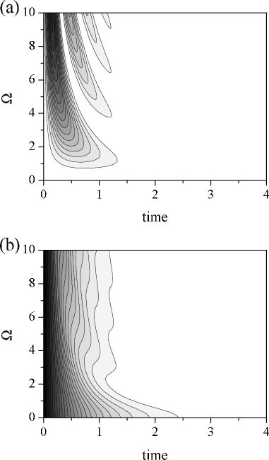
Figure 1: (a) $\zeta$ and (b) $\chi$ as a function of the Rabi frequency and time for $T_{1}=1.5$, $T_{2}=0.5$, and $\tilde{R}_{3}=0$. For all figures the darkest shading corresponds to 0.20 for $\zeta$–plots, and 20 increasing lighter shadings are used until $\zeta=0$. For $\chi$–plots the darkest shading corresponds to 1 and 20 increasing lighter shadings are used until $\chi=0.5$.

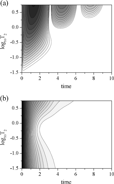
Figure 2: (a) ${\rm Log}_{10}\ \!\zeta$ and (b) $\chi$ as a function of $\log_{10}T_{2}$ and time for $T_{1}=2.5$, and $\tilde{R}_{3}=0$. The upper limit of the ordinate scale corresponds to $T_{2}=T_{1}/2$, as in Eq. (4). For all the $\log_{10}\ \!\zeta$–plots the darkest shading corresponds to $\zeta=0.30$, and 20 increasing lighter shadings are used until $\zeta=0.0003$.

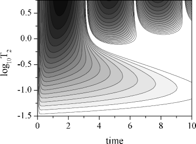
Figure 3: ${\rm Log}_{10}\ \!\zeta$ as a function of $\log_{10}T_{2}$ and time for $T_{1}=10^{4}$, and $\tilde{R}_{3}=0$. The upper limit on the ordinate is as in Fig. 2.

Figure 4: $\rho_{11}(t)$ for three different values of the Rabi frequency: $\Omega=0.2$ (solid line), $\Omega=1$ (dashed line), and $\Omega=5$ (dotted line). To compare, two different values of $T_{1}$ are considered (with $T_{2}=0.5$): (a) $T_{1}=2.5$ and (b) $T_{1}=10^{4}$. In (c), $\rho_{11}(t)$ for three different values of $T_{2}$ (with $T_{1}=10^{4}$ and $\Omega=1$): $T_{2}=0.05$ (solid line), $T_{2}=0.5$ (dashed line), and $T_{2}=5$ (dotted line).

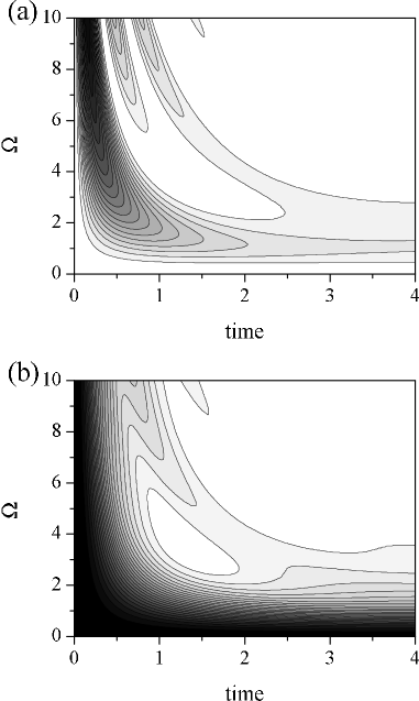
Figure 5: (a) $\zeta$ and (b) $\chi$ as a function of the Rabi frequency and time for $T_{1}=1.5$, $T_{2}=0.5$, and $\tilde{R}_{3}=1$.

Figure 6: (a) $\chi$, (b) $\zeta$, and (c) $\rho_{11}$ for three different values of the Rabi frequency: $\Omega=0.5$ (solid line), $\Omega=\Omega_{r}=1.15$ (dashed line), and $\Omega=4$ (dotted line). In all cases: $\tilde{R}_{3}=1$, $T_{1}=1.5$, $T_{2}=0.5$.