Quantum adiabatic evolutions that can’t be used to design efficient algorithms

Abstract

Quantum adiabatic computation is a novel paradigm for the design of quantum algorithms, which is usually used to find the minimum of a classical function. In this paper, we show that if the initial hamiltonian of a quantum adiabatic evolution with a interpolation path is too simple, the minimal gap between the ground state and the first excited state of this quantum adiabatic evolution is an inverse exponential distance. Thus quantum adiabatic evolutions of this kind can’t be used to design efficient quantum algorithms. Similarly, we show that a quantum adiabatic evolution with a simple final hamiltonian also has a long running time, which suggests that some functions can’t be minimized efficiently by any quantum adiabatic evolution with a interpolation path.

Quantum computation has attracted a great deal of attention in recent years, because some quantum algorithms show that the principles of quantum mechanics can be used to greatly enhance the efficiency of computation. Recently, a new novel quantum computation paradigm based on quantum adiabatic evolution has been proposed FGGS00 . We call quantum algorithms of this paradigm quantum adiabatic algorithms. In a quantum adiabatic algorithm, the evolution of the quantum register is governed by a hamiltonian that varies continuously and slowly. At the beginning, the state of the system is the ground state of the initial hamiltonian. If we encode the solution of the algorithm in the ground state of the final hamiltonian and if the hamiltonian of the system evolves slowly enough, the quantum adiabatic theorem guarantees that the final state of the system will differ from the ground state of the final hamiltonian by a negligible amount. Thus after the quantum adiabatic evolution we can get the solution with high probability by measuring the final state. For example, Grover’s algorithm has been implemented by quantum adiabatic evolution in RC02 . Recently, the new paradigm for quantum computation has been tried to solve some other interesting and important problems RAO03 ; DKK02 ; TH03 ; TDK01 ; FGG01 .

Usually, except in some simple cases, a decisive mathematical analysis of a quantum adiabatic algorithm is not possible, and frequently even the estimation of the running time is very difficult. Sometimes we have to conjecture the performance of quantum adiabatic algorithms by numerical simulations, for example in FGG01 . In this paper, we estimate the running time of a big class of quantum adiabatic evolutions. This class of quantum adiabatic evolutions have a simple initial hamiltonian and a universal final hamiltonian. We show that the running time of this class of quantum adiabatic evolutions is exponential of the size of problems. Thus they can’t be used to design efficient quantum algorithms. We noted that E. Farhi et al. have got the similar result by a continuous-time version of the BBBV oracular proof BBBV97 in FGGN05 . However, our proof is based on the quantum adiabatic theorem, which is much simpler and more direct. Furthermore, our result can be generalized from the case of linear path to the case of interpolation paths. Besides, by the symmetry of our proof it is easy to prove that a quantum adiabatic evolution that has a simple final hamiltonian and a universal final hamiltonian also has a long running time, which can be used to estimate the worst performance of some quantum adiabatic algorithms.

For convenience of the readers, we briefly recall the local adiabatic algorithm. Suppose the state of a quantum system is $|\psi(t)\rangle(0\leq t\leq T)$, which evolves according to the Schrödinger equation

$$i\frac{d}{dt}|\psi(t)\rangle=H(t)|\psi(t)\rangle,$$ (1)

where $H(t)$ is the Hamiltonian of the system. Suppose $H_{0}=H(0)$ and $H_{1}=H(T)$ are the initial and the final Hamiltonians of the system. Then we let the hamiltonian of the system vary from $H_{0}$ to $H_{1}$ slowly along some path. For example, a interpolation path is one choice,

$$H(t)=f(t)H_{0}+g(t)H_{1},$$ (2)

where $f(t)$ and $g(t)$ are continuous functions with $f(0)=g(T)=1$ and $f(T)=g(0)=0$ ($T$ is the running time of the evolution). Let $|E_{0},t\rangle$ and $|E_{1},t\rangle$ be the ground state and the first excited state of the Hamiltonian at time t, and let $E_{0}(t)$ and $E_{1}(t)$ be the corresponding eigenvalues. The adiabatic theorem LIS55 shows that we have

$$|\langle E_{0},T|\psi(T)\rangle|^{2}\geq 1-\varepsilon^{2},$$ (3)

provided that

$$\frac{D_{max}}{g_{min}^{2}}\leq\varepsilon,\ \ \ \ 0<\varepsilon\ll 1,$$ (4)

where $g_{min}$ is the minimum gap between $E_{0}(t)$ and $E_{1}(t)$

$$g_{min}=\min_{0\leq t\leq T}[E_{1}(t)-E_{0}(t)],$$ (5)

and $D_{max}$ is a measurement of the evolving rate of the Hamiltonian

$$D_{max}=\max_{0\leq t\leq T}|\langle\frac{dH}{dt}\rangle_{1,0}|=\max_{0\leq t\leq T}|\langle E_{1},t|\frac{dH}{dt}|E_{0},t\rangle|.$$ (6)

Before representing the main result, we give the following lemma.

Lemma 1

Suppose $f:\{0,1\}^{n}\rightarrow R$ is a function that is bounded by a polynomial of n. Let $H_{0}$ and $H_{1}$ be the initial and the final hamiltonians of a quantum adiabatic evolution with a linear path $H(t)$. Concretely,

$$H_{0}=I-|\alpha\rangle\langle\alpha|,$$ (7)

$$H_{1}=\sum\limits_{z=1}^{N}{f(z)|z\rangle\langle z|},$$ (8)

$$H(t)=(1-t/T)H_{0}+(t/T)H_{1},$$ (9)

where, $T$ is the running time of the quantum adiabatic evolution and

$$|\alpha\rangle=|\hat{0^{n}}\rangle=\frac{1}{\sqrt{N}}\sum\limits_{i=1}^{N}{|i\rangle},\ \ N=2^{n}.$$ (10)

Then we have

$$g_{min}<\frac{2}{2^{n/2-n/100}}.$$ (11)

Thus $T$ is exponential in $n$.

Proof. Let

$$H(s)=(1-s)(I-|\alpha\rangle\langle\alpha|)+s\sum\limits_{z=1}^{N}{f(z)|z\rangle\langle z|},$$

where $s=t/T$. Suppose $\{f(z),1\leq z\leq N\}=\{a_{i},1\leq i\leq N\}$ and $a_{1}\leq a_{2}\leq...\leq a_{N}$. Without loss of generality, we suppose $a_{1}=0$. Otherwise we can let

$$H(s)=H(s)-I\times\min_{1\leq i\leq N}a_{i},$$ (12)

which doesn’t change $g_{min}$ of $H(s)$. We also suppose $a_{i}<a_{i+1},1<i<N-1$(Later we will find that this restriction can be removed).

Now we consider $A(\lambda)$, the characteristic polynomial of $H(s)$. It can be proved that

$$A(\lambda)= \prod_{i=1}^{N}{(1-s-\lambda+sa_{i})}$$ (13)

$$-\frac{1-s}{N}\sum_{j=1}^{N}{\prod_{k\neq j}^{D}{(1-s-\lambda+sa_{k})}}.$$ (14)

For every $s\in(0,1)$, we have $A(0)>0$ and $A(1-s)<0$. Because $A(\lambda)$ is a polynomial, $A(\lambda)$ has a root $\lambda_{1}(s)$ in the interval $(0,1-s)$. Similarly, in each of the intervals $(1-s+sa_{k},1-s+sa_{k+1})(1\leq k\leq N-1)$ there is a root $\lambda_{k+1}(s)$. It can be proved that in the interval $(0,\lambda_{1}(s))$, $A(\lambda)>0$. Otherwise if for some $\lambda_{0}\in(0,\lambda_{1}(s))$, $A(\lambda_{0})<0$, there will be another root in the interval $(0,\lambda_{0})$. In this case the number of the eigenvalues of $H(s)$ is more than $N$, which is a contradiction. Similarly we have $A(\lambda)<0$ for interval $(\lambda_{1}(s),\lambda_{2}(s))$ and we have $A(\lambda)>0$ for interval $(\lambda_{2}(s),1-s+sa_{2})$.

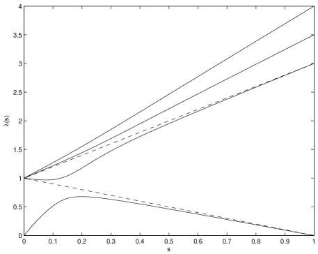
Figure 1: The two dashed lines are $\lambda(s)=1-s$ and $\lambda(s)=1-s+sa_{2}$, and the solid lines are the four lowest eigenvalue curves of $H(s)$, where $N=16$, $a_{1}=0$, and $a_{i}=2+i/2$ for $1<i\leq 16$.

Consider a line $\lambda_{2}^{{}^{\prime}}(s)=1-(1-1/m)s$ in the $s$-$\lambda(s)$ plane, where $m=poly(n)$ or a positive polynomial in n. Suppose we can find a $m$ that $a_{2}>1/m$ for every $n$ big enough. Then we know that for every big $n$, the line $\lambda_{2}^{{}^{\prime}}(s)$ lies in the region between lines $\lambda=1-s$ and $\lambda=1-s+sa_{2}$. By solving the inequation $A(1-(1-1/m)s)<0$ we can get which part of the line $\lambda_{2}^{{}^{\prime}}(s)$ lies in the region between lines $\lambda=1-s$ and the eigenvalue curve $\lambda_{2}(s)$. The result is, when $s\in(0,s_{2})$ the line $\lambda_{2}^{{}^{\prime}}(s)$ lies above $\lambda_{2}(s)$ and when $s\in(s_{2},1)$ the eigenvalue curve $\lambda_{2}(s)$ lies above $\lambda_{2}^{{}^{\prime}}(s)$, where

$$s_{2}=\frac{1}{1+\frac{N}{\sum\limits_{j=1}^{N}{\frac{1}{a_{j}-\frac{1}{m}}}}}.$$ (15)

Similarly, we consider another line $\lambda_{1}^{{}^{\prime}}(s)=1-(1+1/m)s$. By similar analysis, we get that when $s\in(0,s_{1})$ the line $\lambda_{1}^{{}^{\prime}}(s)$ lies above $\lambda_{1}(s)$ and when $s\in(s_{1},1)$ the eigenvalue curve $\lambda_{1}(s)$ lies above $\lambda_{1}^{{}^{\prime}}(s)$, where

$$s_{1}=\frac{1}{1+\frac{N}{\sum\limits_{j=1}^{N}{\frac{1}{a_{j}+\frac{1}{m}}}}}.$$ (16)

It can be proved that for any fixed positive polynomial $m$

$$s_{1}<s_{2}$$ (17)

if $n$ is big enough. Now we consider the interval $(s_{1},s_{2})$. In this interval, the eigenvalues curves $\lambda_{1}(s)$ and $\lambda_{2}(s)$ all lies between the lines $\lambda_{1}^{{}^{\prime}}(s)$ and $\lambda_{2}^{{}^{\prime}}(s)$. At the same time, it is easy to know that the gap between the lines $\lambda_{1}^{{}^{\prime}}(s)$ and $\lambda_{2}^{{}^{\prime}}(s)$ is less than $2/m$. Thus the minimal gap between $\lambda_{1}(s)$ and $\lambda_{2}(s)$ is also less than $2/m$. That is to say,

$$g_{min}<2/m.$$ (18)

Obviously, to get Eq.(17) the restriction $a_{2}>1/m$ above can be removed, because if $a_{2}<1/m$, the gap between $\lambda_{1}(s)$ and $\lambda_{2}(s)$ is less than $1/m$ when $s$ is near 1, then we also have Eq.(17). Furthermore, the restriction $a_{i}<a_{i+1},1<i<N-1$ can also be removed. If $a_{i}=a_{i+1}$ for some $i$, we can give a very small disturbance to $H_{1}$, which make every $a_{i}$ different, while $g_{min}$ doesn’t change too much (for example, we can let the change of $g_{min}$ much less than $1/m$).

Similarly, Supposing $m=2^{n/2-n/100}$, we also have $s_{1}<s_{2}$ if $n$ is big enough. At this time, for any $s\in(s_{1},s_{2})$ the gap between $\lambda_{1}(s)$ and $\lambda_{2}(s)$ is less than $\frac{2}{2^{n/2-n/100}}$. So we have

$$g_{min}<\frac{2}{2^{n/2-n/100}}.$$ (19)

In fact, 100 in Eq.(18) can be replaced by any big natural number. By the quantum adiabatic theorem, the running time of this quantum adiabatic evolution is exponential in $n$. That completes the proof of this lemma. $\Box$

Lemma 1 shows that, to find the minimum of the function $f(x)$ effectively using the quantum adiabatic algorithms, the initial hamiltonian $H_{0}$ can’t be too simple (See also FGGN05 ). If we set the initial hamiltonian according to the structure of the function $f(x)$, the effect maybe better. For example in section 7.1 of DMV01 ,

$$H_{0}=\sum\limits_{z\in\{0,1\}^{n}}{w(z)|\hat{z}\rangle\langle\hat{z}|},$$ (20)

and

$$H_{1}=\sum\limits_{z\in\{0,1\}^{n}}{w(z)|z\rangle\langle z|},$$ (21)

where $H_{0}$ is diagonal in the Hadamard basis with the bit values

$$|\hat{0}\rangle=\frac{1}{\sqrt{2}}(|0\rangle+|1\rangle),\ \ |\hat{1}\rangle=\frac{1}{\sqrt{2}}(|0\rangle-|1\rangle),$$ (22)

and $w(z)=z_{1}+z_{2}+...+z_{n}$. In this quantum adiabatic evolution, the initial hamiltonian reflect the structure of the function that we want to minimize. $g_{min}$ of this evolution is independent of $n$, and the quantum algorithm consisted by this evolution is efficient.

Noted that Lemma 1 shows that the time complexity of the quantum adiabatic algorithm for the hidden subgroup problem proposed in RAO03 is exponential in the number of input qubits RAO06 . Similarly, the main result of ZH06 can also be got again via Lemma 1, which was also pointed out in FGGN05 .

In Lemma 1, the path of quantum adiabatic evolutions is linear. The following theorem shows that this can be generalized.

Theorem 1

Suppose $H_{0}$ and $H_{1}$ given by Eq. (7) and Eq. (8) are the initial and the final hamiltonians of a quantum adiabatic evolution. Suppose this quantum adiabatic evolution has a interpolation path

$$H(t)=f(t)H_{0}+g(t)H_{1}.$$ (23)

Here $f(t)$ and $g(t)$ are arbitrary continuous functions, subject to the boundary conditions

$$f(0)=1\ \ \ g(0)=0,$$ (24)

$$f(T)=0\ \ \ g(T)=1,$$ (25)

and

$$c_{1}<f(t)+g(t)<c_{2},\ \ 0\leq t\leq T,$$ (26)

where, $T$ is the running time of the adiabatic evolution and $c_{1}$ and $c_{2}$ are positive real numbers. Then we have

$$g_{min}<\frac{2c_{2}}{2^{n/2-n/100}}.$$ (27)

Thus $T$ is exponential in $n$.

Proof. Note that

$$H(t)=(f(t)+g(t))(\frac{f(t)}{f(t)+g(t)}H_{0}+\frac{g(t)}{f(t)+g(t)})H_{1},$$ (28)

and $\frac{f(t)}{f(t)+g(t)}$ is a continuous functions whose range of function is $[0,1]$. Suppose the gap of the ground state and the first excited state of the quantum adiabatic evolution $H^{\prime}(t)=(1-t/T)H_{0}+(t/T)H_{1}$ arrives at its minimum at $t_{0}\in[0,T]$, then the corresponding gap of $H(t)$ at $t^{\prime}_{0}$ will be less than $\frac{2c_{2}}{2^{n/2-n/100}}$, where $\frac{g(t^{\prime}_{0})}{f(t^{\prime}_{0})+g(t^{\prime}_{0})}=t_{0}/T$.

That completes the proof of this Theorem. $\Box$

We have shown that a simple initial hamiltonian is bad for a quantum adiabatic evolution. Similarly, a simple final hamiltonian is also bad. First we represent the following lemma.

Lemma 2

Suppose $f:\{0,1\}^{n}\rightarrow R$ is a function that is bounded by a polynomial of n. Let $H_{0}$ and $H_{1}$ are the initial and the final hamiltonians of a quantum adiabatic evolution with a linear path $H(t)$. Concretely,

$$H_{0}=\sum\limits_{z=1}^{N}{f(z)|\hat{z}\rangle\langle\hat{z}|},$$ (29)

$$H_{1}=I-|x\rangle\langle x|,\ \ 1\leq x\leq N,$$ (30)

$$H(t)=(1-t/T)H_{0}+(t/T)H_{1},$$ (31)

where, $H_{0}$ is diagonal in the Hadamard basis and $T$ is the running time of the quantum adiabatic evolution. Then we have

$$g_{min}<\frac{2}{2^{n/2-n/100}}.$$ (32)

Thus $T$ is exponential in $n$.

Proof. Let

$$H^{\prime}(s)=(1-s)H_{1}+sH_{0},$$

and

$$H^{\prime\prime}(s)=(H^{\bigotimes n})H^{\prime}(s)(H^{\bigotimes n}),$$

where $s=t/T$ and $H$ is the Hadamard gate. First, by symmetry it’s not difficult to prove that $H^{\prime}(s)$ and $H(s)$ have the same $g_{min}$. Second, $H^{\prime}(s)$ and $H^{\prime\prime}(s)$ have the same characteristic polynomial, then they also have the same $g_{min}$. So the $g_{min}$ of $H^{\prime\prime}(s)$ is the minimal gap that we want to estimate. On the other hand, it also can be proved that $H^{\prime\prime}(s)$ has the same characteristic polynomial as Eq.(13) no matter what $x$ is. Thus according to Lemma 1 we can finish the proof. $\Box$

Analogously, Lemma 2 can also be generalized to the case of interpolation paths.

Theorem 2

Suppose $H_{0}$ and $H_{1}$ given by Eq. (28) and Eq. (29) are the initial and the final hamiltonians of a quantum adiabatic evolution. Suppose this quantum adiabatic evolution has a interpolation path

$$H(t)=f(t)H_{0}+g(t)H_{1}.$$ (33)

Here $f(t)$ and $g(t)$ are arbitrary continuous functions, subject to the boundary conditions

$$f(0)=1\ \ \ g(0)=0,$$ (34)

$$f(T)=0\ \ \ g(T)=1,$$ (35)

and

$$c_{1}<f(t)+g(t)<c_{2},\ \ 0\leq t\leq T,$$ (36)

where, $T$ is the running time of the adiabatic evolution and $c_{1}$ and $c_{2}$ are positive real numbers. Then we have

$$g_{min}<\frac{2c_{2}}{2^{n/2-n/100}}.$$ (37)

Thus $T$ is exponential in $n$.

If $f(z)$ arrives at its minimum when $z=z_{0}$ and if for any $z\neq z_{0}$ $f(z)$ has the same value, Eq.(8) will have a form similar Eq.(29). Theorem 2 shows that if we use a quantum adiabatic evolution with a interpolation path to minimize a function of this kind, the running time will be exponential in $n$ no matter what $H_{0}$ is. For example, in quantum search problem $f(z)$ is of this form. Again we show that quantum computation can’t provide exponential speedup for search problems. Furthermore, Theorem 2 can help us with other problems. For some quantum adiabatic algorithms, we may use it to consider the possible worst case. If in some case $f(z)$ only has two possible values and arrives at the minimum at only one point, we can say that the worst case performance of the quantum adiabatic algorithm with a interpolation path that minimizes $f(z)$ is exponential.

In conclusion, we have shown in a quantum adiabatic algorithm if the initial hamiltonian or the final hamiltonian is too simple, the performance of the algorithm will be very bad. Thus, we have known that when designing quantum algorithms, some quantum adiabatic evolutions are hopeless. Furthermore, we also know that for some function $f(z)$, we can’t use any quantum adiabatic algorithm with a interpolation path to minimize it effectively.

References

- (1) E. Farhi, J. Goldstone, S. Gutmann, and M. Sipser, e-print quant-ph/0001106.
- (2) J. Roland and N. J. Cerf, Phys. Rev. A 65, 042308(2002).
- (3) Tad Hogg, Phys. Rev. A 67, 022314(2003).
- (4) T. D. Kieu, e-print quant-ph/0110136.
- (5) S. Das, R. Kobes, G. Kunstatter, Phys. Rev. A 65, 062310(2002).
- (6) M. V. Panduranga Rao, Phys. Rev. A 67, 052306(2003).
- (7) E. Farhi et al. e-print quant-ph/0104129.
- (8) C. H. Bennett, E. Bernstein, G. Brassard and U. V. Vazirani, SIAM J. Comput. 26, 1510-1523(1997).
- (9) E. Farhi, J. Goldstone, S. Gutmann, and D. Nagaj, e-print quant-ph/0512159.
- (10) L. I. Schiff, Quantum Mechanics (McGraw-Hill, Singapore, 1955).
- (11) W. van Dam, M. Mosca and U. V. Vazirani, FOCS 2001, 279-287.
- (12) M. V. Panduranga Rao, Phys. Rev. A 73, 019902(E)(2006).
- (13) M.Znidaric and M. Horvat, Phys. Rev. A 73, 022329(2006).