Thermal limitation of far-field matter-wave interference

Abstract

We assess the effect of the heat radiation emitted by mesoscopic particles on their ability to show interference in a double slit arrangement. The analysis is based on a stationary, phase-space based description of matter wave interference in the presence of momentum-exchange mediated decoherence.

I Introduction

A recent demonstration of the wave nature of large-sized molecules with a high internal temperature Hackermuller2003a (1) poses the question on the ultimate physical limitations for the observation of matter wave interference with increasingly macroscopic particles Schlosshauer2006a (2). The present article focuses on one of the basic effects known to destroy the coherence of matter waves, namely the heat radiation emitted by the particles themselves. We take these objects to be sufficiently complex so that their internal state calls for a thermodynamic description and obtain the general scaling behavior as a function of their temperature, heat capacity, and effective surface area.

As a second motive, we note that the loss of coherence in a two-path matter wave interferometer has been the subject of a number of recent studies, discussing various models and mechanisms FacchiNonsense (3, 4, 5, 6, 7, 8, 9). All of those treatments employ a temporal description of the decohering dynamics, usually by approximately solving a master equation or a corresponding stochastic differential equation. Here we present an alternative way of dealing with decoherence of matter wave beams, which is based on describing the rate of decoherence events and their effect separately. Using the Wigner-Weyl formulation of quantum mechanics one finds how the stationary scattering state of the particle beam gets affected by momentum-exchange mediated decoherence. This way a clear and transparent description of the underlying physics is obtained.

We consider the most basic situation of far-field interference where a stationary beam of matter waves passes a double slit arrangement, although the treatment is easily generalized to multi-slit gratings. The application to the case of heat radiation yields simple, yet experimentally relevant formulas for the expected loss of the interference contrast, and permits to incorporate and discuss important issues such as the effects of cooling and and of deviations from the ideal blackbody spectrum.

The experimental studies of the impact of light emission on matter waves started with the scattering of laser beams off interfering atoms Pfau1994a (10, 11, 12). More recently, the decohering effect of the continuous, Planck-like heat radiation emitted by fullerenes was observed, in agreement with decoherence theory, in the near-field regime of Talbot-Lau interference Hackermuller2004a (13, 14). Theoretical discussions of the general effect of heat radiation serving to “localize” a spatially extended quantum state into a mixture of more local states can be found in Joos1985a (15, 16, 17, 18, 19, 20), though not in the context of interferometry.

The structure of the article is as follows. Section 2 starts by collecting the required equations to treat general momentum-exchange mediated decoherence. Since the approach was already used in Hornberger2004a (21) to treat the related case of near-field interference we keep the presentation short. Section 3 proceeds to calculate the double slit far-field interference pattern in the presence of decoherence. Based on this we discuss the visibility reduction due to heat radiation, i.e., the thermal limitation for interference, with mesoscopic particles in Sect. 4. Quantitative estimates are presented for carbonaceous aerosols, and compared to the case of fullerene molecules. The article concludes with with Sect. 5.

II Decoherence mediated by momentum transfer

The ability of a particle to show interference may be reduced due the interaction and entanglement with unobserved degrees of freedom, such as collisions with particles from a background gas or the absorption and emission of photons. It is often justified, and consistent with the Markov assumption, to model this loss of coherence as due to individual events, which occur probabilistically and independently of each other. The situation is particularly simple if the motional state of the particle $\hat{\varrho}^{\prime}$, obtained by tracing over the unobserved degrees of freedom, depends only on the momentum exchange during the event. In position representation, the off-diagonal elements are then merely reduced by a complex factor $\eta$, with $\left|\eta\right|\leqslant 1$. The reduction depends only on the corresponding distance,

$$\langle\boldsymbol{R}_{1}|\hat{\varrho}^{\prime}|\boldsymbol{R}_{2}\rangle = \langle\boldsymbol{R}_{1}|\hat{\varrho}|\boldsymbol{R}_{2}\rangle\,\eta\left(\boldsymbol{R}_{1}-\boldsymbol{R}_{2}\right),$$ (1)

while the diagonal elements are unaffected, $\eta\left(0\right)=1$. This loss of coherence can be attributed to the amount of which-way information revealed to the environment after the interaction Arndt2005a (22). At the same time, the “decoherence function” $\eta$ is given by the Fourier transform of the probability density for the momentum exchange, $\eta\left(\Delta\boldsymbol{R}\right)=\eta^{\ast}\left(-\Delta\boldsymbol{R}\right)={\int\,\mathrm{d}^{3}\boldsymbol{Q}\exp\left(i\Delta\boldsymbol{R}\cdot\boldsymbol{Q}/\hbar\right)\overline{\eta}\left(\boldsymbol{Q}\right)},$ which is manifest in the operator representation of (1),

$$\hat{\varrho}^{\prime} = \int\,\mathrm{d}^{3}\boldsymbol{Q}\,\bar{\eta}\left(\boldsymbol{Q}\right)\mathrm{e}^{i\widehat{\mathsf{R}}\cdot\boldsymbol{Q}/\hbar}\,\hat{\varrho}\,\mathrm{e}^{-i\widehat{\mathsf{R}}\cdot\boldsymbol{Q}/\hbar}.$$ (2)

In fact, in the more general framework of translation-invariant and completely positive master equations the function $\eta$ can be related to the characteristic function of the relevant Poissonian part of the corresponding Lévy process Vacchini2005a (23). For later reference we note that in terms of the Wigner function the state change (2) reads

$$W^{\prime}\left(\boldsymbol{R},\boldsymbol{P}\right) = \int\mathrm{d}^{3}\boldsymbol{Q}\,\bar{\eta}\left(\boldsymbol{Q}\right)W\left(\boldsymbol{R},\boldsymbol{P}-\boldsymbol{Q}\right).$$ (3)

The time evolution equation for the resulting decohering motion is obtained immediately from (1) if one assumes that the decoherence events occur with a rate $\gamma\left(t\right)$. It has the Markovian form $\partial_{t}\hat{\varrho}=\left(i\hbar\right)^{-1}[\widehat{\mathsf{H}},\hat{\varrho}]+\mathcal{L}_{t}\hat{\varrho}$, with the incoherent part given by

$$\langle\boldsymbol{R}_{1}|\mathcal{L}_{t}\hat{\varrho}|\boldsymbol{R}_{2}\rangle = -\gamma\left(t\right)\left[1-\eta\left(\boldsymbol{R}_{1}-\boldsymbol{R}_{2}\right)\right]\langle\boldsymbol{R}_{1}|\hat{\varrho}|\boldsymbol{R}_{2}\rangle.$$

The process of decoherence by the emission of heat radiation fits into the present framework provided the particle beam is unpolarized and the density of the electro-magnetic field modes can be taken constant in space, i.e., if the modification of the emission rate due to nearby surfaces can be neglected. If the walls of the apparatus are located far away compared to the photon wave length the sole effect of a photon emission on the motional state of the particle is an isotropic momentum kick (the internal degrees of freedom remain in a separable state). One obtains the corresponding decoherence function by expressing the probability density for a photon to be emitted at (angular) frequency $\omega$ in terms of the temperature dependent spectral photon emission rate $R_{\omega}\left(\omega;T\right)$. The result is

$$\eta\left(\boldsymbol{R}\right) = \frac{1}{R_{\operatorname{tot}}}\int_{0}^{\infty}\mathrm{d}\omega R_{\omega}\left(\omega;T\right)\operatorname{sinc}\left(\frac{\omega}{c}\left|\boldsymbol{R}\right|\right)$$ (5)

with total emission rate $R_{\operatorname{tot}}=\int_{0}^{\infty}\mathrm{d}\omega R_{\omega}\,\left(\omega;T\right)$ and $\operatorname{sinc}\left(x\right)\equiv\sin\left(x\right)/x.$ Putting aside this particular form we keep $\eta$ unspecified in the following section, thereby including all other (possibly anisotropic) momentum-transfer mediated decoherence mechanisms.

III Decoherence in double slit interference

III.1 Phase space description of double slit interference

We proceed to formulate the double-slit interference of matter waves in the phase space representation (e.g., Ozorio1998a (24, 25)). This will permit us to incorporate the effect of decoherence in the subsequent section.

Consider the usual interferometric situation with a well-collimated, stationary beam of particles directed in the positive $z$-direction. Noting that the stationarity implies the absence of coherences between different longitudinal momenta Rubenstein1999b (26), it is represented by a (non-normalizable) state where the longitudinal and transverse motion are initially separable,

$$\hat{\varrho}_{\operatorname{in}} = \int\mathrm{d}p_{z}\,g\left(p_{z}\right)\hat{\rho}\left(p_{z}\right)\otimes|p_{z}\rangle\langle p_{z}|,$$ (6)

with $g\left(p_{z}\right)$ the longitudinal momentum distribution function and $\hat{\rho}$ a transverse state. Since this is a convex sum we can at first take the incoming state of the beam to have a well-defined longitudinal velocity $p_{z}/m$, and discuss the effect of a finite longitudinal coherence length later. Lower-case vectors are used to denote coordinates in the transverse plane, e.g., $\boldsymbol{r}\equiv\left(x,y,0\right)$. Accordingly, the Wigner function of the transverse motion is given by

$$w\left(\boldsymbol{r},\boldsymbol{p}\right) = \frac{1}{\left(2\pi\hbar\right)^{2}}\int\mathrm{d}^{2}\boldsymbol{q}\,\mathrm{e}^{-i\boldsymbol{r}\cdot\boldsymbol{q}/\hbar}\,$$

$$\phantom{\frac{1}{\left(2\pi\hbar\right)^{2}}\int}\times\langle\boldsymbol{p}-\frac{\boldsymbol{q}}{2}|\hat{\rho}\left(p_{z}\right)|\boldsymbol{p}+\frac{\boldsymbol{q}}{2}\rangle.$$

Now, if the passage through a single pinhole rendered the transverse motion in the pure state $|\psi_{\text{s}}\rangle$ a double slit arrangement with identical pinholes would produce the state

$$|\psi_{0}\rangle = \frac{1}{\sqrt{2}}\left(e^{i\hat{\mathsf{p}}\cdot\boldsymbol{d}/2\hbar}+e^{-i\hat{\mathsf{p}}\cdot\boldsymbol{d}/2\hbar}\right)|\psi_{\text{s}}\rangle,$$ (8)

provided there is full transverse coherence over the double slit separation $\boldsymbol{d}$. As implied by the normalization, we take the translated pinhole states to be non-overlapping, $\langle\psi_{\text{s}}|e^{-i\hat{\mathsf{p}}\cdot\boldsymbol{d}/\hbar}|\psi_{\text{s}}\rangle=0$. Allowing for arbitrary pinhole states $\hat{\rho}_{\text{s}}$ the relation (8) reads $\hat{\rho}_{0}=2\cos\left(\hat{\mathsf{p}}\cdot\boldsymbol{d}/2\hbar\right)\hat{\rho}_{\text{s}}\cos\left(\hat{\mathsf{p}}\cdot\boldsymbol{d}/2\hbar\right)$, and accordingly we have in phase space representation:

$$w^{\left(0\right)}\left(\boldsymbol{r},\boldsymbol{p}\right) = \frac{1}{2}w^{\left(\text{s}\right)}\left(\boldsymbol{r}+\frac{\boldsymbol{d}}{2},\boldsymbol{p}\right)+\frac{1}{2}w^{\left(\text{s}\right)}\left(\boldsymbol{r}-\frac{\boldsymbol{d}}{2},\boldsymbol{p}\right).$$ (9)

$$+\cos\left(\frac{\boldsymbol{p}\cdot\boldsymbol{d}}{\hbar}\right)w^{\left(\text{s}\right)}\left(\boldsymbol{r},\boldsymbol{p}\right).$$

This implies that the probability density of the transverse momentum is related to the corresponding single slit distribution $w_{p}^{\left(\text{s}\right)}\left(\boldsymbol{p}\right):=\int\mathrm{d}^{2}\boldsymbol{r}\,w^{\left(s\right)}\left(\boldsymbol{r},\boldsymbol{p}\right)$ by

$$w_{p}^{\left(0\right)}\left(\boldsymbol{p}\right) := \int\mathrm{d}^{2}\boldsymbol{r}\,w^{\left(0\right)}\left(\boldsymbol{r},\boldsymbol{p}\right)=$$ (10)

$$= \left[1+\cos\left(\frac{\boldsymbol{p}\cdot\boldsymbol{d}}{\hbar}\right)\right]w_{p}^{\left(\text{s}\right)}\left(\boldsymbol{p}\right).$$

The great advantage of the phase space representation shows up in the the free evolution from the double slit, at $z=0$ to the screen located at $z=L$, since the corresponding states are related by the free shearing transformation (e.g. Hornberger2004a (21))

$$w^{\left(L\right)}\left(\boldsymbol{r},\boldsymbol{p}\right)=w^{\left(0\right)}\left(\boldsymbol{r}-L\frac{\boldsymbol{p}}{p_{z}},\boldsymbol{p}\right).$$ (11)

With this one arrives at the familiar result that the interference pattern in the far field is given by the momentum distribution of the particle state after it passed the grating,

$$w^{\left(L\right)}_{r}\left(\boldsymbol{r}\right) := \int\mathrm{d}^{2}\boldsymbol{p}\,w^{\left(L\right)}\left(\boldsymbol{r},\boldsymbol{p}\right)$$ (12)

$$= \frac{p_{z}^{2}}{L^{2}}\int\mathrm{d}^{2}\boldsymbol{r}_{0}\,w^{\left(0\right)}\left(\boldsymbol{r}_{0},p_{z}\frac{\boldsymbol{r}-\boldsymbol{r}_{0}}{L}\right)$$

$$\cong \frac{p_{z}^{2}}{L^{2}}\int\mathrm{d}^{2}\boldsymbol{r}_{0}\,w^{\left(0\right)}\left(\boldsymbol{r}_{0},p_{z}\frac{\boldsymbol{r}}{L}\right)\hskip 10.00002pt\text{for $\left|\boldsymbol{r}\right|\gg\left|\boldsymbol{d}\right|$}$$

$$= \frac{p_{z}^{2}}{L^{2}}w_{p}^{\left(0\right)}\left(p_{z}\frac{\boldsymbol{r}}{L}\right).$$

As the only approximation we used here that $w^{\left(0\right)}\left(\cdot,\boldsymbol{p}_{0}\right)$ is localized in the small pinhole areas so that one can neglect the $p_{z}\boldsymbol{r}_{0}/L$ term for for $\left|\boldsymbol{r}\right|\gg\left|\boldsymbol{d}\right|$. This is equivalent to the far-field approximation of Fraunhofer diffraction. Insertion of the momentum distribution after the double slit yields the far field pattern

$$w^{\left(L\right)}_{r}\left(\boldsymbol{r}\right) = \frac{p_{z}^{2}}{L^{2}}\left[1+\cos\left(\frac{p_{z}}{L}\frac{\boldsymbol{r}\cdot\boldsymbol{d}}{\hbar}\right)\right]w_{p}^{\left(\text{s}\right)}\left(p_{z}\frac{\boldsymbol{r}}{L}\right),$$ (13)

and it shows the expected modulation of the single slit momentum distribution by interference fringes with a period of $2\pi\hbar L/\left(p_{z}\left|\boldsymbol{d}\right|\right)=\lambda_{\text{dB}}L/\left|\boldsymbol{d}\right|$. It is common to attribute a visibility of $\mathcal{V}=1$ to this pattern.

In experiments, one typically uses detectors, which measure the intensity of the interference pattern (the number of particles per unit area and time). In addition, one should take into account that molecular beams cannot be prepared in a monochromatic state, but have a finite longitudinal coherence. By allowing for a distribution of the longitudinal momenta $g\left(p_{z}\right)$ the expected intensity is proportional to

$$I\left(\boldsymbol{r}\right) = \int\mathrm{d}p_{z}\,g\left(p_{z}\right)\,\frac{p_{z}}{m}w^{\left(L\right)}_{r}\left(\boldsymbol{r}\right).$$ (14)

However, to keep the formulation simple we take a fixed value of $p_{z}$ in the following, and note that the general case is simply recovered by weighting the resulting intensities with $g\left(p_{z}\right)$. In any case, for the beams used in molecular interferometry we can safely assume the contributing $p_{z}$ to be much larger than the possible longitudinal momentum transfers, so that the change of the velocity due to photon emission can be neglected in the following section, where we proceed to account for decoherence.

III.2 Incorporating decoherence

At first sight, the obvious way to incorporate the effect of decoherence would be to solve the corresponding master equation (LABEL:eq:me). As shown in Sect. VI. of Ref. Hornberger2004a (21), a systematic scheme can indeed be set up which yields successive approximations of the corresponding time evolution in a closed form. However, by insisting on a dynamic description to treat an inherently stationary problem one loses much transparency in the formulation. This renders a stationary treatment much more appropriate, as will be clear in the following.

Let us first consider the impact of a single decoherence event occurring at some longitudinal position $z$. The interference pattern conditioned on this event is obtained by propagating the state to position $z$ with (11), performing the decohering convolution (3), and a further propagation to the final screen position $L$. It follows that the resulting intensity pattern is given by

$$I^{\prime}\left(z;\boldsymbol{r}\right) = \frac{p_{z}}{m}\int\mathrm{d}^{2}\boldsymbol{q}\,\mathrm{d}q_{z}\int\mathrm{d}^{2}\boldsymbol{p}\,\bar{\eta}\left(\boldsymbol{q}+q_{z}\boldsymbol{e}_{z}\right)$$

$$\times w^{\left(0\right)}\left(\boldsymbol{r}-L\frac{\boldsymbol{p}}{p_{z}}+z\frac{\boldsymbol{q}}{p_{z}},\boldsymbol{p}-\boldsymbol{q}\right)$$

$$\cong \,\frac{p_{z}^{3}}{mL^{2}}\int\mathrm{d}^{2}\boldsymbol{q}\,w^{\left(0\right)}_{p}\left(p_{z}\frac{\boldsymbol{r}}{L}-\frac{L-z}{L}\boldsymbol{q}\right)$$

$$\times\int\mathrm{d}q_{z}\,\bar{\eta}\left(\boldsymbol{q}+q_{z}\boldsymbol{e}_{z}\right)$$

$$= \int\mathrm{d}^{2}\boldsymbol{q}I\left(\boldsymbol{r}-\frac{L-z}{p_{z}}\boldsymbol{q}\right)\int\mathrm{d}q_{z}\,\bar{\eta}\left(\boldsymbol{q}+q_{z}\boldsymbol{e}_{z}\right).$$

Here we performed the same far-field approximation as above in (12), took into account that only $\left|q_{z}\right|\ll p_{z}$ contribute in $\bar{\eta}$, and related the result to the unperturbed intensity pattern (14). In the same fashion, one finds that additional decoherence events are described by further convolutions with $\bar{\eta}$.

The trick is now to consider the differential equation which governs the change of the interference pattern as one increases the longitudinal interval where decoherence events may occur. This is straightforward since the patterns are related by a convolution. After taking the Fourier transform of the interference pattern, $\bar{I}\left(\boldsymbol{q}\right)=\left(2\pi\hbar\right)^{-2}{\int\mathrm{d}^{2}\boldsymbol{r}\exp\left(-i\boldsymbol{r}\cdot\boldsymbol{q}/\hbar\right)I\left(\boldsymbol{r}\right)}\,$, the relation (LABEL:eq:Iprime) turns into a multiplication with the decoherence function,

$$\bar{I}^{\prime}\left(z;\boldsymbol{q}\right) = \bar{I}\left(\boldsymbol{q}\right)\eta\left(\frac{z-L}{p_{z}}\boldsymbol{q}\right).$$ (16)

We denote by $\Gamma_{z}\left(z\right)\mathrm{d}z$ the (possibly position dependent) average number of decoherence events occurring in $\left(z,z+\mathrm{d}z\right)$. The differential change of the pattern is then determined by

$$\frac{\mathrm{d}}{\mathrm{d}z}\bar{I}_{\operatorname{dec}}\left(z;\boldsymbol{q}\right) = \Gamma_{z}\left(z\right)\left[\bar{I}_{\operatorname{dec}}\left(z;\boldsymbol{q}\right)\eta\left(\boldsymbol{q}\frac{z-L}{p_{z}}\right)\right.$$

$$\left.\phantom{\Gamma_{z}\left(z\right)\left[\right.}-\bar{I}_{\operatorname{dec}}\left(z;\boldsymbol{q}\right)\right].$$

The integration from $z=0$ to $z=L$ yields

$$\bar{I}_{\operatorname{dec}}\left(\boldsymbol{q}\right) = \exp\left[-\int_{0}^{L}\,\mathrm{d}z\Gamma_{z}\left(z\right)\left(1-\eta\left(\boldsymbol{q}\frac{z-L}{p_{z}}\right)\right)\,\right]$$ (18)

$$\times\bar{I}\left(\boldsymbol{q}\right).$$

After a final Fourier transform we obtain the general result

$$I_{\operatorname{dec}}\left(\boldsymbol{r})\right. = \int\mathrm{d}^{2}\boldsymbol{s}\,h\left(\boldsymbol{s}\right)I\left(\boldsymbol{r}-\boldsymbol{s}\right)\,.$$ (19)

It shows that the entire effect of decoherence on the interference pattern is described by a convolution with the real kernel

$$h\left(\boldsymbol{s}\right) := \frac{1}{\left(2\pi\hbar\right)^{2}}\int\mathrm{d}^{2}\boldsymbol{q}\,\mathrm{e}^{i\boldsymbol{q}\cdot\boldsymbol{s}/\hbar}$$

$$\times\exp\left[-\int_{0}^{L}\,\mathrm{d}z\,\Gamma_{z}\left(z\right)\left(1-\eta\left(\boldsymbol{q}\frac{z-L}{p_{z}}\right)\right)\,\right].$$

It is determined by the decoherence function from (1) and the (possibly time-dependent) rate of decoherence events $\gamma\left(t\right)$, related to $\Gamma_{z}$ by $\Gamma_{z}\left(z\right)v_{z}=\gamma\left(z/v_{z}\right)$ with $v_{z}=p_{z}/m$. (The fact that (19) is positive for all intensity patterns $I\left(\boldsymbol{r}\right)$ follows with Bochner’s theorem by noting that the exponential function in (18) is of positive type since $\eta$ is of positive type.) It should be emphasized that multiple decoherence events are treated correctly in this description, provided they are statistically independent, since (III.2) is a linear equation.

Note that the result (19), (III.2) is valid for any initial momentum distribution $w_{p}^{\left(0\right)}$ thus covering arbitrary multi-slit interference arrangements. If we go back to the case of a double slit (13) an approximate, but very intuitive form is obtained if the width of $w^{\left(\text{s}\right)}_{p}$ is so large that one can pull the envelope of the interference pattern out of the $\boldsymbol{s}$-integration. If we also take $\eta$ to be isotropic (and therefore real) the interference pattern reads in this case

$$I_{\operatorname{dec}}\left(\boldsymbol{r})\right. \cong \frac{v_{z}p_{z}^{2}}{L^{2}}\left[1+\mathcal{V}\cos\left(\frac{p_{z}}{\hbar}\frac{\boldsymbol{r}\cdot\boldsymbol{d}}{L}\right)\right]w^{\left(\text{s}\right)}_{p}\left(p_{z}\frac{\boldsymbol{r}}{L}\right).$$

It differs from the unperturbed pattern, see (13), by the factor

$$\mathcal{V} = \exp\left[-\frac{1}{v_{z}}\int_{0}^{L}\,\mathrm{d}z\,\gamma\left(\frac{z}{v_{z}}\right)\left(1-\eta\left(\boldsymbol{d}\frac{L-z}{L}\right)\right)\,\right],$$

which reduces the oscillating term. Although there is no unique definition for the visibility of a non-periodic signal like (LABEL:eq:Idec2), one may call this the visibility reduction due to decoherence.

Equation (LABEL:eq:Vred) has a particularly intuitive form since it involves the separation of the two interfering paths in the argument of the decoherence function. Close to the double-slit, at $z=0$, the decoherence function enters with the full slit separation $\left|\boldsymbol{d}\right|$. As the particle approaches the screen the two paths get closer, requiring an increasingly large “resolving power” of the decoherence events if they are to contribute to the visibility reduction by conveying some which way information. At the screen, where $z=L$ and $\eta\left(0\right)=1$ the paths coalesce and decoherence has no effect. This dependence on the longitudinal position has been observed in experiments where a laser beam was scattered off interfering atoms Pfau1994a (10, 11, 12), albeit in a Mach-Zehnder setup. It is also an important factor in the quantitative description of the recent near-field experiment on decoherence by heat radiation Hackermuller2004a (13).

Note that in the case of near-field Talbot-Lau interference an approximate expression for the visibility reduction has been found in Ref. Hornberger2004a (21). It is similar to (LABEL:eq:Vred), but the denominator in the argument of of $\eta$ is replaced by (an integer fraction of) the Talbot length $d^{2}/\lambda_{\operatorname{dB}}$. While this underlines the strength of the phase space approach in incorporating decoherence in the various regimes of interferometry, we note that the intermediate case, where neither near-field nor far-field approximations hold, is more complicated.

IV Thermal scaling behavior

Based on the results of the preceding section we can now study at what temperatures the wave nature of material objects ceases to be observable due to their heat radiation. For a start, it should be noted that, strictly speaking, one can apply (LABEL:eq:Vred) only if the thermal photons are emitted in a Poisson process, which would require the particle to be permanently in contact with a heat bath. The isolated, mesoscopic particle-waves traversing the interferometer are typically not in thermal equilibrium with the surrounding radiation field, and they are characterized by the amount of energy stored in their many internal degrees of freedom. One may express this internal energy in terms of the micro-canonical temperature $T$ and the heat capacity $C_{V}$.

As a consequence of the absence of a proper heat bath each photon emission reduces the micro-canonical temperature by $\hbar\omega/C_{V}$. This modifies the emission probability of the subsequent photons and renders the process non-Poissonian. However, in an approximate description the main consequences of this this effect can be accounted for by an inhomogeneous Poisson process with a time-dependent emission rate $\gamma\left(t\right)=R_{\operatorname{tot}}\left(T\left(t\right)\right)$ where $T\left(t\right)$ is determined by the cooling equation $\partial_{t}T\left(t\right)=-\int\mathrm{d}\omega\,\hbar\omega R_{\omega}\left(\omega;T\left(t\right)\right)/C_{V}$. One writes (LABEL:eq:Vred) as a time integration and inserts (5) which cancels the $R_{\operatorname{tot}}$ dependence. The resulting visibility reduction due to heat radiation reads

$$\mathcal{V} = \exp\left[-\int_{0}^{\tau}\,\mathrm{d}t\int_{0}^{\infty}\mathrm{d}\omega R_{\omega}\left(\omega;T\left(t\right)\right)\right.$$

$$\left.\phantom{\exp\left[\right.}\times\left\{1-\operatorname{sinc}\left(\frac{\omega d}{c}\left(1-\frac{t}{\tau}\right)\right)\right\}\right]$$

with $\tau:=L/v_{z}$ the time of flight and $d=\left|\boldsymbol{d}\right|$ the slit separation. Likewise, the corresponding full intensity pattern is obtained by replacing the exponential in the kernel (III.2) with the right hand side of (IV), after the substitution $d\rightarrow\left|\boldsymbol{q}\right|L/p_{z}$. As discussed above, the calculation of this modified pattern is required if one has to account for a finite coherence length.

As exemplified below, the influence of cooling can be quite significant in realistic scenarios. For objects with a molecular structure it is even more crucial to account for the full frequency dependence of the emission rate. The reason is that the rate is strongly affected by the electronic excitation spectrum of the molecule, which typically shows a gap at optical to near infrared frequencies, leading to a much stronger temperature and frequency dependence than expected for a blackbody radiator.

In the following we consider interfering objects which are still considerably larger than molecules, so that the absorption cross section $\sigma_{\operatorname{abs}}$ can be taken frequency and temperature independent and proportional to the surface area $\mathcal{A}$. Although this is unrealistic for molecules, it is quite reasonable for submicrometer particles like aerosols or large proteins, which display an essentially featureless absorption cross section in the relevant frequency regime Bohren1983a (27). In this case one accounts for the deviations with respect to the macroscopic blackbody spectrum by introducing the emissivity $\varepsilon$, which characterizes the effective emission area $\mathcal{A}_{\varepsilon}:=\varepsilon\mathcal{A}$. The spectral photon emission rate is then given by Hansen1998a (28)

$$R_{\omega}\left(\omega,T\right) = \frac{\mathcal{A}_{\varepsilon}\omega^{2}}{\left(2\pi c\right)^{2}}\exp\left(-\frac{\hbar\omega}{k_{\text{B}}T}-\frac{k_{B}}{2C_{V}}\left(\frac{\hbar\omega}{k_{\text{B}}T}\right)^{2}\right).$$

The statistical factor differs here from the usual Bose-Einstein distribution function because the particle is not in thermal equilibrium with the colder, surrounding radiation field, so that induced absorption plays no role. The term involving the heat capacity is present since the emission reduces the internal energy.

Solving the cooling equation with the emission spectrum (LABEL:eq:Rarea) one finds that the particle temperature decreases like $T\left(t\right)=T_{0}[1+T_{0}^{3}/T^{3}_{\inf}\left(t\right)]^{-1/3}$. Here, the limiting temperature at time $t$ is determined by $T_{\inf}^{-3}\left(t\right)=9k_{\text{B}}^{4}\mathcal{A}_{\varepsilon}tF\left(C_{V}/k_{B}\right)/\left(2\pi^{2}c^{2}\hbar^{3}C_{V}\right)$ where the factor $F\left(x\right)=1-10x^{-1}+105x^{-2}+\mathcal{O}\left(x^{-3}\right)$ accounts for the $C_{V}$-dependence in (LABEL:eq:Rarea). Below, this result is used to give a quantitative estimate for aerosols.

As a final step, we take the particle to be truly macroscopic in the sense that the heat capacity is so large that the effect of cooling can be neglected, $C_{V}/k_{\text{B}}\rightarrow\infty$. It follows from (IV) that the visibility then decays exponentially with the time of flight, i.e., $\mathcal{V}=\exp\left(-\tau/\tau_{\operatorname{th}}\right)$. The characteristic decoherence time $\tau_{\operatorname{th}}$ is determined by a spectral integration involving the sine integral $\operatorname{Si}(x)$ Abramowitz1965a (29),

$$\tau_{\operatorname{th}}^{-1} = \int_{0}^{\infty}\mathrm{d}\omega R_{\omega}\left(\omega;T\right)\left[1-\frac{c}{\omega d}\operatorname{Si}\left(\frac{\omega d}{c}\right)\right].$$ (25)

With the special choice (LABEL:eq:Rarea) for the emission rate the integral can be done. One obtains the final result for the decoherence time

$$\tau_{\operatorname{th}}^{-1} = \frac{\mathcal{A}_{\varepsilon}c}{\left(2\pi\right)^{2}d^{3}}f\left(\frac{k_{\text{B}}Td}{\hbar c}\right)$$ (26)

with the scaling function

$$f\left(x\right) = 2x^{3}-\frac{x^{3}}{1+x^{2}}-x^{2}\arctan\left(x\right).$$

The expansion for small arguments renders the reciprocal decoherence time proportional to the square of the slit separation $d$ and to the fifth power of the temperature $T$, or Matsubara frequency,

$$\tau_{\operatorname{th}}^{-1} = \frac{1}{3\pi^{2}}\frac{\mathcal{A}_{\varepsilon}d^{2}}{c^{4}}\left(\frac{k_{\text{B}}T}{\hbar}\right)^{5}\times\left[1+\mathcal{O}\left(\frac{k_{\text{B}}Td}{\hbar c}\right)^{2}\right].$$ (27)

Within this approximation the kernel (III.2) for the blurred interference pattern attains a particularly simple form. It turns into a Gaussian of unit area whose width $\sigma_{s}$ is given by of $\sigma^{2}_{s}=2m{\mathcal{A}_{\varepsilon}\left(k_{\text{B}}T\right)^{5}\left(L/\hbar p_{z}\right)^{3}}/\left(3\pi^{2}c^{4}\right)$.

It should be emphasized that the decoherence time $\tau_{\operatorname{th}}$ is expedient only with respect to the particular interferometric context. Given a choice for the time of flight $L/v_{z}$ and the grating separation $d$, it determines the temperature beyond which the wave nature of the particle ceases to be observable.

Note also that decoherence was considered to occur only between the double slit and the detector, so far. In the same manner one may incorporate decoherence events taking place in front of the double slit, although this depends on the details of how the transverse coherence is produced. It is straightforward if a single, narrow “coherence slit” is placed in front of the double slit. The effect is then given by a second convolution of the form (19), with $L$ in the kernel replaced by the distance between coherence slit and double slit. If those distances are equal one just has to multiply the right-hand side of Eqs. (25), (26), and (27) by the factor of 2.

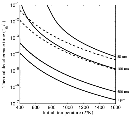
Figure 1: Thermal decoherence time for double slit interference as a function of the initial particle temperature. The curves correspond to a slit separation $d$ of 50 nm, 100 nm, 500 nm, and 1 $\mu$m (top to bottom). The solid lines incorporate the effect of cooling as described by (IV) and (LABEL:eq:Rarea), while the dashed lines show the result (26) for an asymptotically large heat capacity (they are indistinguishable for $d=500\,\operatorname{nm},1\,\mu m$). The particle parameters $\mathcal{A}_{\varepsilon}=5\times 10^{-18}\text{m}^{2}$ and $C_{V}=12000k_{\text{B}}$ correspond to ultrafine carbonaceous aerosols, as discussed in the text.

Figure 1 shows the decoherence time $\tau_{\operatorname{th}}$, i.e., the time of flight where the visibility reduces to $\mathcal{V}=\mathrm{e}^{-1}$ as calculated by a numerical inversion of (IV), together with the limiting result (26) (dashed lines). They are given as a function of the initial temperature and for several slit separations $d$. Our choice of the two particle parameters, the effective surface area $\mathcal{A}_{\varepsilon}$ and the heat capacity $C_{V}$, is given in the caption. These values correspond to ultra-fine carbonaceous aerosols. They were obtained by assuming a particle mass of 10⁵ amu, a density of 10³ kg/m³, a specific heat capacity of 10³ J/(kg K), and a mass specific absorption cross section of 7.5$\times$10³ m²/kg as reported in Bond2006a (30).

One observes in Fig. 1 that the decoherence times depend strongly on the slit separation and on the temperature. This is due to the fact that a thermal photon emission can be harmful to interference only if its wave length is sufficiently small to (partially) resolve the path separation by carrying which-path information to the environment. The rate of these harmful events decreases with decreasing temperature, which raises the permissible time of flight, i.e., the de Broglie wave length of the particle beam. The difference between the solid lines and dashed lines in Fig. 1 shows that the effect of cooling can be relevant even for the considered mesoscopic particles. In particular for small slit separations, which are much more easily coherently illuminated, the harmful photons carry so much energy that the probability of further harmful emissions is substantially diminished. This leads to a rather strong increase of $\tau_{\operatorname{th}}$ with respect to the limiting result (the dashed lines). Only for separations around 500   nm the two descriptions start to be indistinguishable.

It must be emphasized that the above results for mesoscopic particles do not apply to large molecules, such as fullerenes, even if they display a continuous thermal radiation spectrum. This can be seen in Fig. 2 which shows the decoherence times for a beam of C₇₀ fullerene molecules. The data was obtained by numerically integrating the cooling equation and inverting (IV), using empirical data for the frequency-dependent absorption cross section, as discussed in Hornberger2005a (14). One observes that considerably larger temperatures are required to induce decoherence times comparable to those of Fig. 1. More importantly, the mesoscopic result (26), indicated by the dotted lines, cannot yet be applied, not even for a qualitative description of the curves.

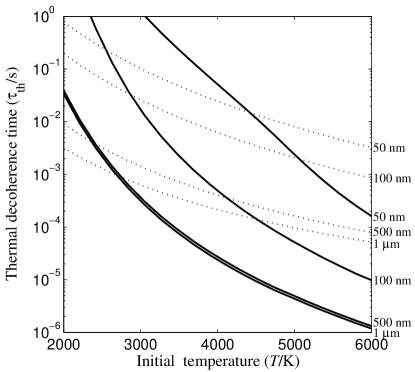
Figure 2: Thermal decoherence time for double slit interference with fullerene molecules. The solid lines were calculated from Eq. (IV) using the full frequency- and cooling-dependent emission rate. Compared to Fig. 1, similar decoherence times are found only at considerably larger temperatures. The comparison with the dotted lines shows that for fullerenes the mesoscopic result (26) is not yet applicable, not even for a qualitative description of the temperature dependence of the interference contrast ($\mathcal{A}_{\varepsilon}=10^{-22}$ m² Kolodney1995b (31)).

It is remarkable that the slit separations of $d=500\,\operatorname{nm}$ and of $d=1\,\mu m$ display an almost equal dependence on thermal decoherence. This behavior is due to the gap in the electronic excitation spectrum of fullerenes, which strongly suppresses radiation above about $800\,\operatorname{nm}$. As a consequence, interference with slit separations beyond that length is affected similarly by the emitted photons. It should also be emphasized that the effect of cooling is much stronger than in the case of Fig. 1. Its neglect would render the decoherence times larger by an order of magnitude for $d=50\,\operatorname{nm}$, and still about threefold larger for $d=1\,\mu m$ (not shown). This is part of the reason why the present results differ markedly from those of Ref. FacchiNonsense (3), which account neither for the effect of cooling nor for the detailed emission spectrum of fullerenes .

V Conclusions

The present article described the effect of momentum-exchange mediated decoherence on far-field interference of material waves. Rather than solving the dynamic equation of motion, a phase space formulation for the stationary scattering problem was employed. This way exact and transparent expressions could be derived for the modification of the interference pattern due to the presence of decoherence. Although we specialized to the case of double slit interference, the generalization to arbitrary multi-slit arrangements is straightforward in the present formulation.

We calculated the reduction of the interference visibility due to the particle’s heat radiation and found that a realistic description of molecular objects requires accounting for the effect of cooling and for the particle color, i.e., the deviations from the blackbody behavior. A particularly simple scaling behavior could be obtained for mesoscopic particles, which are characterized only by their emissivity and heat capacity.

As a final point, let us illustrate the temperature requirements for an object of the size of a small virus, assuming a mass of $5\times 10^{7}\,\operatorname{amu}$. The rivaling effect of collisional decoherence was estimated for such a particle to limit the permissible pressure of background gases to $p_{0}=2.7\times 10^{-11}\,\operatorname{mbar}\left(\tau/\text{s}\right)^{-1}$ Colldeco (32). Using the above-mentioned mass-specific absorption cross section Bond2006a (30) we find from (27) that the characteristic temperature is as low as $T_{0}={19\,\text{K}\,\left(d^{2}\tau/\mu\text{m}^{2}\text{s}\right)^{-1/5}}$. Inserting reasonable values for the slit separation and the time of flight, $d=0.5\,\mu\text{m}$ and $\tau=0.1\,\text{s}$, this yields about 40   K. It indicates that the thermal decoherence may be more difficult to control than the effect of background gases for particles of that size. It must be emphasized, however, that in the foreseeable future interferometry of mesoscopic objects will be limited by the practical difficulty of producing brilliant particle beams and of avoiding vibrational noise Stibor2005a (33), rather than by the “natural” decoherence mechanism of heat radiation.

Acknowledgments

Helpful discussions with Markus Arndt are gratefully acknowledged. This work was supported by the DFG Emmy Noether program.

References

- (1) L. Hackermüller, S. Uttenthaler, K. Hornberger, E. Reiger, B. Brezger, A. Zeilinger, and M. Arndt, Phys. Rev. Lett. 91, 90408 (2003).
- (2) M. Schlosshauer, Ann. Phys. (N.Y.) 321, 112–149 (2006).
- (3) P. Facchi, A. Mariano, and S. Pascazio, Recent Res. Devel. Physics 3, 1–29 (2002); P. Facchi, S. Pascazio, and T. Yoneda, eprint quant-ph/0509032 (2005).
- (4) A. Viale, M. Vicari, and N. Zanghi, Phys. Rev. A 68, 063610 (2003).
- (5) Y. Levinson, J. Phys. A: Math. Gen. 37, 3003–3017 (2004).
- (6) A. S. Sanz, F. Borondo, and M. J. Bastiaans, Phys. Rev. A 71, 042103 (2005).
- (7) F. C. Lombardo, F. D. Mazzitelli, and P. I. Villar, Phys. Rev. A 72, 042111 (2005).
- (8) P. Machnikowski, quant-ph/0511022 (2005).
- (9) T. Qureshi and A. Venugopalan, eprint quant-ph/0602052 (2006).
- (10) T. Pfau, S. Spälter, C. Kurtsiefer, C. Ekstrom, and J. Mlynek, Phys. Rev. Lett. 73, 1223–1226 (1994).
- (11) M. S. Chapman, T. D. Hammond, A. Lenef, J. Schmiedmayer, R. A. Rubenstein, E. Smith, and D. E. Pritchard, Phys. Rev. Lett. 75, 3783 – 3787 (1995).
- (12) D. A. Kokorowski, A. D. Cronin, T. D. Roberts, and D. E. Pritchard, Phys. Rev. Lett. 86, 2191 (2001).
- (13) L. Hackermüller, K. Hornberger, B. Brezger, A. Zeilinger, and M. Arndt, Nature 427, 711–714 (2004).
- (14) K. Hornberger, L. Hackermüller, and M. Arndt, Phys. Rev. A 71, 023601 (2005).
- (15) E. Joos and H. D. Zeh, Z. Phys. B. 59, 223–243 (1985).
- (16) W. H. Zurek, Phys. Today 44(10), 36 (1991).
- (17) M. Tegmark, Found. Phys. Lett. 6, 571–590 (1993).
- (18) D. Dürr and H. Spohn, Decoherence Through Coupling to the Radiation Field, in Lecture Notes in Physics, volume 538, pages 77–86, Springer, Heidelberg, 1999.
- (19) R. Alicki, Phys. Rev. A 65, 034104 (2002).
- (20) E. Joos, H. D. Zeh, C. Kiefer, D. Giulini, J. Kupsch, and I.-O. Stamatescu, Decoherence and the Appearance of a Classical World in Quantum Theory, Springer, Berlin, 2nd edition, 2003.
- (21) K. Hornberger, J. E. Sipe, and M. Arndt, Phys. Rev. A 70, 053608 (2004).
- (22) M. Arndt, K. Hornberger, and A. Zeilinger, Physics World 18(3), 35–40 (2005).
- (23) B. Vacchini, Phys. Rev. Lett. 95, 230402 (2005).
- (24) A. M. Ozorio de Almeida, Phys. Rep. 295, 265–342 (1998).
- (25) W. P. Schleich, Quantum Optics in Phase Space, Wiley-VCH, Berlin, 2001.
- (26) R. Rubenstein, A. Dhirani, D. Kokorowski, T. Roberts, E. Smith, W. W. Smith, H. Bernstein, J. Lehner, S. Gupta, and D. Pritchard, Phys. Rev. Lett. 82, 2018–2021 (1999).
- (27) C. E. Bohren and D. R. Huffman, Absorption and Scattering of Light by Small Particles, Wiley, New York, 1983.
- (28) K. Hansen and E. E. B. Campbell, Phys. Rev. E 58, 5477 (1998).
- (29) M. Abramowitz and I. Stegun, Handbook of Mathematical Functions, Dover Publications, New York, 1965.
- (30) T. C. Bond and R. W. Bergstrom, Aerosol. Sci. Technol. 40, 27–67 (2006).
- (31) E. Kolodney, A. Budrevich, and B. Tsipinyuk, Phys. Rev. Lett. 74, 510–513 (1995).
- (32) K. Hornberger, S. Uttenthaler, B. Brezger, L. Hackermüller, M. Arndt, and A. Zeilinger, Phys. Rev. Lett. 90, 160401 (2003); K. Hornberger and J. E. Sipe, Phys. Rev. A 68, 12105 (2003).
- (33) A. Stibor, K. Hornberger, L. Hackermüller, A. Zeilinger, and M. Arndt, Laser Physics 15, 10–17 (2005).