Survival probability of surface excitations in a 2d lattice: non-Markovian effects and Survival Collapse.

Abstract

The evolution of a surface excitation in a two dimentional model is analyzed. I) It starts quadratically up to a spreading time $t_{S}.$ II) It follows an exponential behavior governed by a self-consistent Fermi Golden Rule. III) At longer times, the exponential is overrun by an inverse power law describing return processes governed by quantum diffusion. At this last transition time $t_{R}$ a survival collapse becomes possible, bringing the survival probability down by several orders of magnitude. We identify this strongly destructive interference as an antiresonance in the time domain.

I Introduction

We consider the dynamics of a charge excitation in a typical model for Tamm states DS96 . Similar tight-binding models PM01 are used to describe a variety of situations: molecules absorbed in metallic substrates, decay of high-energy electron excitations and the decoherence caused by a weak interaction with an “environment” whose spectrum is dense. The decay of the survival probability $P_{00}(t)$ of the resulting resonant state is usually described, within a Markovian approximation, by the Fermi Golden Rule (FGR). However, this description contains approximations that leave aside some intrinsically quantum behaviors. Various works on models for nuclei, composite particles Kha58 ; FGR78 ; GMM95 , excited atoms either in a free electromagnetic field FP99 or in photonic lattices KKS94 , showed that the exponential decay has superimposed beats and does not hold for very short and very long times, compared with the lifetime of the system.

In Ref. RP05 we presented a model describing the evolution of a surface excitation in a semi-infinite chain, a model that is solved analytically and susceptible for an experimental test MBS+97 . Here, we present a general analysis showing the quantum nature of the deviations from the Fermi Golden Rule. Then, we numerically solve a model consisting of an excited add atom in a two dimensional lattice. We identify three time regimes in the decay of the survival probability $P_{00}(t)$: 1) For short times the decay is quadratic, as is expected when the coupling of the local state with the continuum is perturbative. 2) An intermediate regime characterized by an exponential behavior, the self-consistent Fermi Golden Rule (SC-FGR) where the rate, the pre-exponential factor and the characteristic frecuency are found self-consistently. 3) A long-time regime in which the exponential decay of the pure survival probability is overrun by an inverse power law, which is identified with the return probability enabled by the slow quantum diffusion in the substrate. At this last cross-over, the oscillations could lead to a dip in $P_{00}(t)$ of several orders of magnitude. This survival collapse is identified with a destructive interference between the pure survival amplitude, i.e., the SC-FGR component, and the return amplitude, associated with high orders in a perturbation theory.

II Survival probability of a surface excitation

We consider the evolution of a surface excitation, prepared in the state $\left|0\right\rangle$ in a Hamiltonian with finite spectrum as is the case of most excitations in a lattice. The survival probability is

$$P_{00}\left(t\right) =\left|\left\langle 0\right|\exp[-\mathrm{i}\hat{H}t/\hbar]\left|0\right\rangle\theta\left(t\right)\right|^{2}$$ (1)

$$\equiv\hbar^{2}\left|G_{00}^{R}\left(t\right)\right|^{2},$$ (2)

where

$$G_{00}^{R}\left(t\right)=\int\frac{\mathrm{d}\varepsilon}{2\pi\hbar}G_{00}^{R}(\varepsilon)\exp[-\mathrm{i}\varepsilon t/\hbar],$$ (3)

is the retarded Green’s function for a single fermion. Expanding the initial condition in the eigenstates of $\hat{H}$ yields KF47 ; Kha58

$$P_{00}(t)=\left|\theta\left(t\right)\int_{-\infty}^{\infty}\mathrm{d}\varepsilon\text{ }N_{0}\left(\varepsilon\right)\exp[-\mathrm{i}\varepsilon t/\hbar]\right|^{2},$$ (4)

where $N_{0}\left(\varepsilon\right)$ is the Local Density of States (LDoS) at site $0$th which, in terms of the retarded Green´s function is $N_{0}\left(\varepsilon\right)=-1/\pi\operatorname{Im}G_{00}^{R}(\varepsilon).$ Hence, we can evaluate the survival probability using the Fourier transform of the LDoS, which can be accurately calculated in the energy representation where the integral is limited to the spectral support. Besides, a clear identification of quantum interferences will be obtained by analyzing the argument of the square modulus.

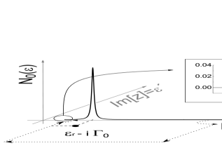
Figure 1: Local spectrum (LDoS) in the complex plane $z=\varepsilon+$i $\varepsilon\acute{}$. $\varepsilon_{L}$ and $\varepsilon_{U}$ are the lower and upper band-edges, respectively. The pole appears in $\varepsilon_{r}-\mathrm{i}\Gamma_{0}.$ The integration path is shown with dotted lines; consist of four straight lines and two arcs, that avoid the band-edges singularities.

In order to evaluate the local dynamics, we perform the integral in Eq.(4) using the residue theorem and following the path shown in the Fig. 1. In the analytical continuation $N_{0}(z)\equiv N_{0}(\varepsilon+\mathrm{i}\varepsilon^{\prime})$, resonances appear as poles in the complex plane. We will consider Hamiltonians where an initially unperturbed state of energy $\varepsilon_{0}=\left\langle 0|\hat{H}|0\right\rangle$ interacting with a continuum is a well defined resonance, i.e., the expansion of $\left|0\right\rangle$ in terms of the eigenstates has a small breath $\Gamma_{0}$ around an energy $\varepsilon_{r}=\varepsilon_{0}+\Delta_{0}$, where $\Delta_{0}=\Delta\left(\varepsilon=\varepsilon_{r}\right)$ is a small shift due to the interaction. We exclude systems with localized eigenstates Ander . Then

$$P_{00}(t) =|\underset{\mathrm{SC-FGR}}{\underbrace{~{}a~{}~{}\mathrm{e}^{-(\Gamma_{0}+\mathrm{i}\varepsilon_{r})t/\hbar}}}$$

$$+\int\limits_{0}^{\infty}\left[\mathrm{e}^{-\left(\varepsilon^{\prime}+\mathrm{i}\text{ }\varepsilon_{L}\right)t/\hbar}N_{0}(\varepsilon_{L}-\mathrm{i}\varepsilon^{\prime})\right.$$

$$\underset{\text{return correction from quantum diffusion}}{\underbrace{\left.-\mathrm{e}^{-\left(\varepsilon^{\prime}+\mathrm{i}\text{ }\varepsilon_{U}\right)t/\hbar}N_{0}(\varepsilon_{U}-\mathrm{i}\varepsilon^{\prime})\right]\text{{d}}\varepsilon^{\prime}}}|^{2},$$ (5)

where

$$a =2\pi\mathrm{i}\lim_{z\rightarrow\varepsilon_{r}-\mathrm{i}\Gamma_{0}}\left[(z-\varepsilon_{r}+\mathrm{i}\Gamma_{0})\text{ }N_{0}(z)\right],$$ (6)

$$=2\pi\mathrm{i}\left[1-\left.\frac{\partial}{\partial\varepsilon}\Delta\left(\varepsilon\right)\right|_{\varepsilon_{r}-\mathrm{i}\Gamma_{0}}\right]^{-1}.$$ (7)

The first term of Eq.(5) already supersedes the usual Fermi Golden Rule approximation since it has a pre-exponential factor ($|a|^{2}\gtrsim 1$) and the exact rate of decay $\Gamma_{0}$. This result is the self-consistent Fermi Golden Rule (SC-FGR). By analogy with a classical Markov model, this exponential term is identified with a “pure survival” amplitude. Within the same analogy, the second term will be called “return” amplitude, as it is fed upon the initial decay. The first term is the dominant one for a wide range of times, while the “quantum diffusion” described by the second, dominates for long times and brings out the details of the spectral structure of the system. The second term is also fundamental for the normalization at very short times where the most excited energy states of the whole system can be virtually explored. Both terms combine to provide the initial quadratic decay required by the perturbation theory:

$$P_{00}\left(t\right)=1-\frac{t^{2}}{\hbar^{2}}\left\langle(\varepsilon-\varepsilon_{r})^{2}\right\rangle_{N_{0}}+\cdots.$$ (8)

Here $\left\langle(\varepsilon-\varepsilon_{r})^{2}\right\rangle_{N_{0}}$ is the energy second moment of the density $N_{0}\left(\varepsilon\right)$. This expansion holds for a time shorter than the spreading time $t_{S}$ of the wave packet formed upon decay.

For long times, the behavior of $P_{00}\left(t\right)$ is governed by the slowly decaying second term in Eq.(5). Only small values of $\varepsilon^{\prime}$ contribute to the integral. This restricts the integration of the LDoS to a range near the band-edges. Then, one can go back to Eq.(4) and perform the Fourier transform retaining only the van Hove singularities SS75 ; FTW76 at these edges. The relative participation of the energy states at each edge of the LDoS is given by the relative weight of the Lorentzian tails at these edges $\beta=[(\varepsilon_{r}-\varepsilon_{L})^{2}+\Gamma_{0}^{2}]/[(\varepsilon_{U}-\varepsilon_{r})^{2}+\Gamma_{0}^{2}].$ Then, the survival probability for long times is

$$P_{00}(t) \approx\left[1+\beta^{2}-2\beta\cos(Bt/\hbar)\right]$$

$$\times\left|\int\text{{d}}\varepsilon^{\prime}\mathrm{e}^{-\varepsilon^{\prime}t/\hbar}N_{0}(\varepsilon_{L}-\mathrm{i}\varepsilon^{\prime})\right|^{2}.$$ (9)

This means that the long time behavior is just the power law decay of the integral multiplied by a factor containing a modulation with frequency $B/\hbar.$

III Survival collapse

In steady state transport DPW89 as well as in dynamical electron transfer LPD90 there are situations when a particle can reach the final state following two alternative pathways. Since each of them collects a different phase, this allows a destructive interference blocking the final state. This phenomenon has been dubbed antiresonance DPW89 ; LPD90 . It extends the Fano resonances describing the anomalous ionization cross-section Fa61 . In the present case, the survival of the local excitation also recognizes two alternative pathways: the pure survival amplitude, which is typically described by the Fermi Golden Rule, and the pathways where the excitation has decayed, explored the substrate, and then returns. These two alternatives can interfere. We rewrite Eq.(5) to emphasize that the survival probability $P_{00}\left(t\right)$ is the result of two different contributions:

$$P_{00}\left(t\right) =\left|\Psi_{S}+\Psi_{R}\right|^{2},$$ (10)

$$=\left|\Psi_{S}\right|^{2}+\left|\Psi_{R}\right|^{2}+2\operatorname{Re}[\Psi_{S}^{\ast}\Psi_{R}],$$ (11)

where the phase in $\Psi_{R}$ arise from the exponentials with $\varepsilon_{L}$ and $\varepsilon_{U}$ (the LDoS is real for any argument). Hence,

$$\Psi_{S}\left(t\right) =\left|a\right|\mathrm{e}^{-\mathrm{i}\phi_{a}}\mathrm{e}^{-\Gamma_{0}t/\hbar}\mathrm{e}^{-\mathrm{i}\left(\varepsilon_{r}-\varepsilon_{L}\right)t/\hbar},$$ (12)

$$\Psi_{R}\left(t\right) =\left|\Psi_{R}\left(t\right)\right|\mathrm{e}^{\mathrm{i}\phi\left(t\right)};$$ (13)

$$\phi\left(t\right) =\arctan\left(\frac{\beta\sin\left(Bt/\hbar\right)}{1-\beta\cos\left(Bt/\hbar\right)}\right).$$ (14)

where Eq.(14) results using the long time limit of Eq.(9). While the interference term in $P_{00}\left(t\right)$ is present along the whole exponential regime, it becomes important when both, the pure survival amplitude and the return contribution, are of the same order. This occurs at the cross-over time $t_{R}$ between the exponential regime and the power law. The interference term can produce a survival collapse, i.e., a pronounced dip that takes $P_{00}\left(t\right)$ close to zero (see Fig. 3). In order to obtain a full collapse, two simultaneous conditions are needed;

$$\left|\Psi_{S}\left(t_{R}\right)\right| =\left|\Psi_{R}\left(t_{R}\right)\right|\text{ \ and \ }$$ (15)

$$\left(\varepsilon_{r}-\varepsilon_{L}\right)t_{R}/\hbar-\phi\left(t_{R}\right) =\left(\pi-\phi_{a}\right)+2\pi n,$$ (16)

which are satisfied with a fair precision because the return amplitude has a phase with a slow variation:

$$\left|\left(\varepsilon_{r}-\varepsilon_{L}\right)/\hbar\right|\gg\Gamma_{0}/\hbar>2\pi/t_{R}\geq\left|\phi\left(t_{R}\right)\right|/t_{R},$$ (17)

while, the pure survival term oscillates rapidly. When both amplitudes are of the same order, the destructive interference will be noticeable.

IV Decay in a 2d-system

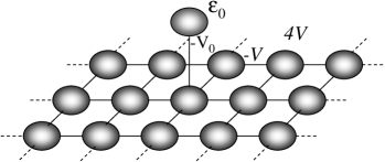
Figure 2: 2d-lattice with an add atom with site energy $\varepsilon_{0}$ and hopping $V_{0}.$

The above results (Eq.(5), Eq.(9), and the survival collapse effect) were verified and quantified in a recent publication RP05 , which solves the dynamics of a surface spin excitation weakly coupled to a semi-infinite chain of interacting spins. The integral in Eq.(4) is analytically solved for the different time regimes (short, exponential and long time). Also, the cross-over from the short time regime to the exponential SC-FGR $t_{S}$, and the cross-over from the SC-FGR to the power law regime $t_{R}$, were found. The survival collapse takes place at $t_{R}$.

Here, we shall consider a square lattice with an add atom. The Tight Binding Hamiltonian is

$$\hat{H}={\displaystyle\sum\limits_{n}}\left|n\right\rangle\varepsilon_{n}\left\langle n\right|-{\displaystyle\sum\limits_{n,m}}\left|n\right\rangle V_{n,m}\left\langle m\right|,$$ (18)

where each $\left\langle r|n\right\rangle$ is centered around the corresponding lattice site $n$, $\varepsilon_{n}$ are the site energies and $V_{n,m}$ are the hoppings. We consider the case where the $0$th site denotes the add atom, i.e., is different from the others sites in both site energy, $\varepsilon_{0}\neq\varepsilon_{n}\equiv 4V$ and hopping $V_{0,1}\equiv V_{0}<V_{n,m}\equiv V$. This defines a continuous spectrum in the range $[0,B\equiv 8V]$. The Green function of this problem, and hence the LDoS, is evaluated using the Dyson equation

$$\left[G_{00}^{R}\left(\varepsilon\right)\right]^{-1}=\left[G_{00}^{R\left(0\right)}\left(\varepsilon\right)\right]^{-1}+V_{0,1}G_{11}^{R\left(0\right)}\left(\varepsilon\right)V_{1,0},$$ (19)

following the general continued fraction procedure described in Ref. PM01 :

$$G_{00}^{R}(\varepsilon)=\frac{1}{\varepsilon-\varepsilon_{0}-V_{0}^{2}G_{11}^{R\left(0\right)}(\varepsilon)},$$ (20)

where $G_{11}^{R\left(0\right)}(\varepsilon)$ is the Green function for a periodic square lattice (Ref. Eco79 ).

For this system, the local second moment of the Hamiltonian is $V_{0}^{2}.$ The short time regime (Eq.(8)) holds up to a time $t_{S}$ in which the quadratic decay becomes an exponential. A good estimate of $t_{S}$ is obtained from the minimal distance between the short time decay and the exponential decay. We can use the first pole approximation (evaluating $G_{11}^{R\left(0\right)}\left(\varepsilon=\varepsilon_{0}\right)$ in Eq.(20)) to obtain $\Gamma_{0}\approx\pi V_{0}^{2}N_{1}^{\left(0\right)}\left(\varepsilon_{0}\right),$ which coincides with the FGR. In the same order of approximation we can take $|a|^{2}\approx 1$ in Eq.(5). Then we obtain

$$t_{S}\approx\hbar\pi N_{1}^{\left(0\right)}\left(\varepsilon_{0}\right).$$ (21)

This result shows that the spreading time $t_{S}$ is only determined by $N_{1}^{\left(0\right)}\left(\varepsilon_{0}\right),$ the local density of states at the first site of the unperturbed substrate.

We verify Eq.(5), Eq.(9), and the survival collapse effect, using the analytical expression for $G_{00}^{R}\left(\varepsilon\right)\$and $N_{0}(\varepsilon),$ and performing the numerical Fourier transform. In Fig. 3 we show $P_{00}(t)$. The curve shows the exponential SC-FGR, which then is overrun by a $1/t^{2}$ power law decay. The cross-over time $t_{R}$ is easily identified through the survival collapse shown as a dip in $P_{00}$. There, the survival probability suddenly decreases from its average by almost three orders of magnitude. The inset shows the small oscillation that modulates the power law.

It is important to note that the square power law decay obtained for long times is a consequence of the $\theta\left(\varepsilon\right)$ dependence of the LDoS (inset of Fig. 1), i.e., this power law is consistent with Eq.(9) taken together with Eq.(20).

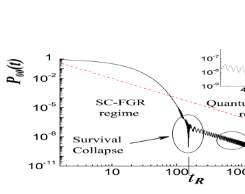
Figure 3: Local polarization, in a doble logarithmic scale, as a function of time. We consider an unperturbed energy of $\varepsilon_{0}/V=2$ and interaction strength $V_{0}/V=0.4.$ This is the case that we consider in Fig.1. The decay exhibits: The exponential behavior as described by the self-consistent Fermi Golden Rule, and an asymptotic square power law decay. The inset shows the oscillation that modulates this decay. The cross-over time $t_{R}$ when the survival collapse takes place is indicated.

V Conclusions

In the present work we have discussed the dynamics of a local excitation that decays through a weak interaction with a continuum spectrum with finite support. Our approach goes beyond the usual Markovian approximation that uses the Fermi Golden Rule to describe these environmental interactions.

The evolution starts with the expected quadratic decay. Then, it follows the usual exponential FGR regime, but with a corrected rate and a pre-exponential factor, i.e., the SC-FGR. Finally, we get the long time regime, that consists of a square power law decay modulated by oscillations whose frequency is determined by the bandwidth. This power law decay is a consequence of the $\theta\left(\varepsilon\right)$ behavior of the LDoS in the band-edge (Eq.(9)) and is identified with the quantum diffusion in the substrate. Hence, anomalies in the excitation decay gives information about the substrate dynamics.

Finally, we predict the existence of the survival collapse. This non-Markovian result fully considers the memory effects to infinite order. Such effect, hinted but not explained in previous works, is visualized as the destructive interference between the pure survival amplitude and the return amplitude that arises from pathways that have already explored the rest of the system.

References

- (1) M. C. Desjonquères and D. Spanjaard, Springer, 2nd Ed. New York, 271 (1996)
- (2) H. M. Pastawski and E. Medina, Rev. Mex. de Fís. 47, 1 (2001), cond-mat/0103219.
- (3) L.A. Khalfin, Sov. Phys. JETP 6, 1053 (1958).
- (4) L. Fonda and G. C. Ghirardi and A. Rimini, Rep. Prog. Phys. 41, 588 (1978).
- (5) G. García Calderón and J.L. Mateos and M. Moshinsky, Phys. Rev. Lett. 74, 337 (1995).
- (6) P. Facchi and S. Pascazio, Phys. A 271, 133 (1999).
- (7) A. G. Kofman and G. Kurizki and B. Sherman, J. Mod. Opt. 41, 353 (1994).
- (8) E. Rufeil-Fiori and H. M. Pastawski, Chem. Phys. Lett. in press, quant-ph/0511176 (2005).
- (9) Z.L. Mádi and B. Brutsher and T. Schulte-Herbrüggen and R. Brüschweiler and R.R. Ernst, Chem. Phys. Lett. 268, 300 (1997).
- (10) N. S. Krylov and V. A. Fock, Zh. Eksp. Teor. Fiz. 17, 93 (1947).
- (11) P. W. Anderson, Rev. of Mod. Phys. 50, 191, section II (1978).
- (12) J.L. D’Amato and H.M. Pastawski and J.F. Weisz, Phys. Rev. B 39, 3554 (1989).
- (13) P.R. Levstein and H.M. Pastawski and J.L. D’Amato, J. Phys. Cond. Matt. 2, 1781 (1990).
- (14) U. Fano, Phys. Rev. 124, 1866 (1961).
- (15) E.N. Economou, Springer Series in Solid State Sciences, 7, Springer-Verlag, New York (1979).
- (16) E-Ni Foo, M. F. Thorpe and D. Weaire, States Surface Science 57, 323 (1976).
- (17) J. R. Schrieffer and P. Soven, Phys. Today 28, issue 4, 24 (1975).