Non-Markovian thermalization of entangled qubits

Abstract

We study the decoherence properties of an entangled bipartite qubit system, represented by two two-level atoms that are individually coupled to non-Markovian reservoirs. This coupling ensures that the dynamical equations of the atoms can be treated independently. The non-Markovian reservoirs are described by a model which leads to an exact non-Markovian master equation of the Nakajima-Zwanzig form [J. Salo, S M. Barnett, and S. Stenholm, Opt. Commun. 259, 772 (2006)]. We consider the evolution of the entanglement of a two-atom state that is initially completely entangled, quantified by its concurrence. Collapses and revivals in the concurrence, induced by the memory effects of the reservoir, govern the dynamics of the entangled quantum system. These collapses and revivals in the concurrence are a strong manifestation of the non-Markovian reservoir.

I Introduction

The dynamics of open quantum systems is usually considered under the assumption that the physical systems of interest are sufficiently isolated from their environment. This allows one to utilize certain approximations such as the weak coupling and the Markovian approximation Breuer . The first approximation ensures that the interaction between the system and the environment is sufficiently weak so that the system is quasi closed. The latter one assumes that the characteristic times of the reservoir are much shorter than that of the system. This allows one to ignore memory effects from the environment and one arrives at time-local equations of motion for the reduced state of the system which are ususally expressed in terms of Gorini-Sudarshan-Kossakowski-Lindblad operators Lindblad ; Gorini . These operators generate a completely positive time evolution which conserve the physical properties of all quantum states Benatti .

Recent studies have shown the limits of the Markovian description of quantum computation and quantum error correction Alicki1 ; Alicki2 ; Ahn1 ; Ahn2 ; Daffer ; Terhal ; Aliferis . In quantum information theory the physical conditions underlying the Markovian approximation can be violated since the coupling of the reduced system to the environment may be of the same order of magnitude as the environment relaxation rate. Consequently, the time evolution of the reduced system is no longer Markovian and the equations of motion either become temporally non-local Nakajima-Zwanzig equations Nakajima ; Zwanzig or explicitly time dependent time-convolutionless equations Shibata , depending on the approach chosen Breuer . A feature that these equations share is that they are often difficult to derive for any given model, and also to solve. Moreover, they may lead to non-physical behavior such as the violation of positivity of the dynamical map Daffer ; Barnett1 ; Budini ; Shabani ; Maniscalco ; Maniscalco2 which is a consequence of the phenomenological nature of most of the non-Markovian approaches. Since there are currently no established criteria that can be used to identify non-Markovian master equations that preserve complete positivity, the only way to ensure this property is to find a model that itself generates completely positive maps and to use it with no approximations in order to derive the final equations of motion. This has recently been achieved by Salo, Barnett and Stenholm Salo by considering the problem of non-Markovian thermal damping of a two-level atom. The model consisted of coupling the principal atom to an additional two-level atom which in turn is coupled to a thermal environment. Utilizing the exact Nakajima-Zwanzig elimination procedure enables them to find a master equation with memory that is guaranteed to generate completely positive evolution.

In this paper we discuss the dynamics of the entanglement of a bipartite system in a non-Markovian reservoir. The system is composed of two qubits which are represented by two-level atoms. In order to derive an exact non-Markovian master equation we extend the model of Salo et al. Salo to an entangled two-atom system to guarantee its completely positive evolution. As in Salo , the two atoms are individually coupled to two additional two-level atoms which in turn interact individually with a thermal environment, as shown in Fig. 1.

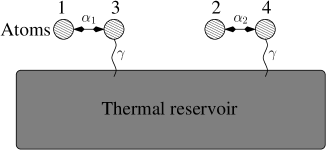
Figure 1: Model for the non-Markovian decay of an entangled two-atom system. Two (entangled) atoms $1$ and $2$ are individually coupled to two additional atoms $3$ and $4$, which are in turn coupled to a thermal reservoir with decay rates $\gamma$.

This ensures that the reservoirs are not able to entangle the two-atom system and, consequently, it is possible to derive non-Markovian master equations which are of a similar form to the equations in Salo . However, although the reservoir is not able to entangle the two-atom systems the dynamics of the entanglement of an initially entangled two-atom system shows a behavior which clearly demonstrates the memory effects of the non-Markovian reservoir. In particular, we show that the entanglement, quantified by the concurrence Wootters1 ; Wootters2 , shows an oscillating behavior in time that depends on the degree to which the reservoir is non-Markovian. Thus, the reservoir remembers that the two-atom system was initially entangled, and the entanglement, which may vanish during the time evolution, can be retrieved by the system, leading to a “collapse and revival like” time evolution of the entanglement. Such an behavior may be of importance in quantum computational systems that are exposed to non-Markovian decoherence effects because even the concurrence of an initially completely entangled state can vanish after a finite period of time Eberly1 ; Eberly2 . Note, however, that the concurrence will partially revive due to the memory of the reservoir that feeds back into the system. Note further, that this model allows decoherence effects to be modified by adjusting the parameters between the interacting atoms. This is to some extent similar to the modification of decoherence Jakob1 ; Jakob2 in engineered reservoirs Monroe1 ; Monroe2 .

The rest of this paper is organized as follows: In Sec. II we introduce the parameterized thermalization model for the entangled qubit system. In Sec. III we derive the dynamical equations of the coupled two-atom system and solve them numerically, assuming that the system is initially in a maximally entangled quantum state of the Bell form. We discuss the dynamical evolution of the entanglement which is quantified by the concurrence, in Sec. IV. We also discuss the effects of a finite-temperature non-Markovian reservoir on the dynamical evolution of the concurrence. We conclude in Sec. V with some discussion.

II Parameterized thermalization model for two entangled qubits

In this section we derive a simple toy model consisting of two entangled qubits that are individually coupled to non-Markovian thermal reservoirs. This model is based on a recently proposed system that consists of a single two-level atom coupled to a specific non-Markovian thermal bath, such that it is possible to derive an exact master equation that preserves complete positivity Salo . The system is composed of a two-level atom $1$ that is coupled via an exchange interaction to another atom $2$, which, in turn, is damped by a thermal reservoir at a specific temperature that can be characterized with the bosonic excitation number $\overline{n}$. We extend this model to an entangled two-atom system $1$ and $2$ where both atoms are assumed to be two-level atoms which are individually coupled to two additional and possibly different two-level atoms $3$ and $4$ via an exchange interaction. The atoms $3$ and $4$ are both damped by a thermal reservoir at a temperature that is characterized with the bosonic excitation number $\overline{n}$. Consequently, the atoms $3$ and $4$ play the role of a “near-environment” to the atoms $1$ and $2$, respectively. Their dynamical influence produces memory effects in the subsystem of atom $1$ and $2$. The individual coupling of the atoms to the reservoir ensures that the dynamics of the two atoms can be treated independently. We note, that in the single-atom case at zero temperature with no initial environment photons present, this system corresponds to the damped Jaynes-Cummings model Barnett , as discussed in Salo .

Suppose the atoms $1$ and $2$ are initially in an arbitrary state. Further, assume that the atoms $3$ and $4$ are initially uncorrelated with the atoms $1$ and $2$ and that they are both in a thermal state

$$\overline{\rho}_{3} = \overline{\rho}_{4}=\overline{\rho}\equiv\left[\begin{array}[]{cc}\frac{\overline{n}}{2\overline{n}+1}&0\\ 0&\frac{\overline{n}+1}{2\overline{n}+1}\end{array}\right].$$ (3)

The initial state of the total system is thus described as

$$\rho(t=0)\equiv\rho_{1234}(t=0)=\rho_{12}(t=0)\otimes\overline{\rho}_{3}\otimes\overline{\rho}_{4}.$$ (4)

Here, $\rho_{12}$ is an arbitrary density operator of the subsystem $1-2$ that allows us to describe initially entangled states of atoms $1$ and $2$. The atomic states represent the computational qubit basis $|0\rangle$ and $|1\rangle$ for the atomic ground and excited state, respectively.

The dynamics of the composite four-atom system is governed by the following equation ($\hbar\equiv 1$)

$$\frac{d\rho(t)}{dt} = -i\left[\sum_{k=1}^{4}H_{k}+H_{\text{int}}^{(13)}+H_{\text{int}}^{(24)},\rho(t)\right]$$ (5)

$$+{\cal{L}}_{3}\rho(t)+{\cal{L}}_{4}\rho(t)$$

$$\equiv {\cal{L}}\rho(t)=[{\cal{L}}^{(1)}+{\cal{L}}^{(2)}]\rho(t),$$

where,

$${\cal{L}}^{(1)} = -i\left[H_{1}+H_{3}+H_{\text{int}}^{(13)},\rho(t)\right]+{\cal{L}}_{3}\rho(t),$$ (6)

$${\cal{L}}^{(2)} = -i\left[H_{2}+H_{4}+H_{\text{int}}^{(24)},\rho(t)\right]+{\cal{L}}_{4}\rho(t),$$ (7)

$$H_{n} = \omega_{n}|1\rangle_{nn}\langle 1|,\qquad n=1,2,3,4$$ (8)

$$H_{\text{int}}^{(13)} = \alpha_{1}\left(\sigma_{1}^{+}\sigma_{3}^{-}+\sigma_{1}^{-}\sigma_{3}^{+}\right),$$ (9)

$$H_{\text{int}}^{(24)} = \alpha_{2}\left(\sigma_{2}^{+}\sigma_{4}^{-}+\sigma_{2}^{-}\sigma_{4}^{+}\right),$$ (10)

$${\cal{L}}_{3}\rho = \gamma(\overline{n}+1)(2\sigma_{3}^{-}\rho\sigma_{3}^{+}-\sigma_{3}^{+}\sigma_{3}^{-}\rho-\rho\sigma_{3}^{+}\sigma_{3}^{-})$$ (11)

$$+\gamma\overline{n}(2\sigma_{3}^{+}\rho\sigma_{3}^{-}-\sigma_{3}^{-}\sigma_{3}^{+}\rho-\rho\sigma_{3}^{-}\sigma_{3}^{+}),$$

$${\cal{L}}_{4}\rho = \gamma(\overline{n}+1)(2\sigma_{4}^{-}\rho\sigma_{4}^{+}-\sigma_{4}^{+}\sigma_{4}^{-}\rho-\rho\sigma_{4}^{+}\sigma_{4}^{-})$$ (12)

$$+\gamma\overline{n}(2\sigma_{4}^{+}\rho\sigma_{4}^{-}-\sigma_{4}^{-}\sigma_{4}^{+}\rho-\rho\sigma_{4}^{-}\sigma_{4}^{+}).$$

Here, $\omega_{n}$, $n=1,2,3,4$ is the energy of the excited state of atom $n$, $\alpha_{1}$ and $\alpha_{2}$ are the coupling strengths between atoms $1-3$ and $2-4$, respectively, $\gamma$ is the thermalization rate for atoms $3$ and $4$, and $\overline{n}$ is the thermal bosonic excitation number. In order to simplify matters we have assumed that the atoms $3$ and $4$ are coupled to a single reservoir, although in principle they could be coupled to separate reservoirs with different temperatures. Note, that the dynamical equation (5) is unable to generate entanglement between the atoms $1$ and $2$ since the equations of motion decouple between the atomic subsystems $1-3$ and $2-4$. However, if entanglement is initially present in the atomic subsystem $1-2$, the memory effects which emerge from the coupling to the atomic subsystems $3$ and $4$ will be able to modify the decoherence rate of the entanglement. Consequently, the non-Markovian bath dynamically influences the decoherence rate of the entanglement of subsystem $1-2$ because of the feedback of the atomic subsystems $3$ and $4$ on the system $1-2$ under consideration.

The underlying idea of this non-Markovian bath model is to assume the atoms $3$ and $4$ serve as “mini-reservoirs” which are able to dynamically modify the equations of motion of the relevant atoms $1$ and $2$. The coupling between the mini-reservoirs can be steered via the interaction parameters $\alpha_{1}$ and $\alpha_{2}$ as well as the detuning parameters $\Delta_{k}=w_{k}-\omega_{k+2}$ for $k=1,2$. These mini-reservoirs will be unobserved and because of their couplings to a thermal Markovian reservoir they are assumed to remain in a certain reference state, namely a thermal reservoir state of a temperature that is imposed by the thermal environment. Their dynamical influence which feeds back into the subsystem $1-2$, however, introduces non-Markovian effects in the atomic subsystem $1-2$. This remains true even in the case when they remain unobserved and are assumed to be in the thermal reference state, as it has been demonstrated in Salo .

The Nakajima-Zwanzig equation of motion Nakajima ; Zwanzig projects the combined quantum system into the relevant parts, described by atom $1$ and $2$, and the irrelevant parts, represented by atoms $3$ and $4$, utilizing projector operators ${\cal{P}}_{k}$ and ${\cal{Q}}_{k}$, where $k=1,2$ indicate the atomic subsystems $1$ and $2$. When we insert the thermal state as the reference state for the atoms $3$ and $4$, the projectors are given as

$${\cal{P}}_{1}\rho_{13} = \text{Tr}_{3}[\rho_{13}]\otimes\overline{\rho}_{3},$$ (13)

$${\cal{P}}_{2}\rho_{24} = \text{Tr}_{4}[\rho_{24}]\otimes\overline{\rho}_{4},$$ (14)

$${\cal{Q}}_{1}\rho_{13} = \rho_{13}-\text{Tr}_{3}[\rho_{13}]\otimes\overline{\rho}_{3},$$ (15)

$${\cal{Q}}_{2}\rho_{24} = \rho_{24}-\text{Tr}_{4}[\rho_{24}]\otimes\overline{\rho}_{4},$$ (16)

where $\rho_{13}$ and $\rho_{24}$ define arbitrary operators (not necessarily density operators) of the atoms $1-3$ and $2-4$, respectively. Note, that in general, the projectors can operate on arbitrary operators of the combined systems $1-3$ and $2-4$. The Nakajima-Zwanzig equation of motion has been derived for the single atom case in Salo under the assumption that, initially, the atom is not entangled with the “mini-reservoir atom” at $t=0$ and the mini-reservoir atom is in the thermal state $\overline{\rho}$. In the two-atom case, the situation which is discussed in this paper, the Nakajima-Zwanzig equations of motion turn out to be of the same form,

$$\frac{d}{dt}{\cal{P}}_{k}\rho^{(k)}(t) = {\cal{P}}_{k}{\cal{L}}^{(k)}{\cal{P}}_{k}\rho^{(k)}(t)$$

$$\!\!\!\!\!\!\!\!+\int_{0}^{t}{\cal{P}}_{k}{\cal{L}}^{(k)}{\cal{G}}^{(k)}(t-\tau){\cal{Q}}_{k}{\cal{L}}^{(k)}{\cal{P}}_{k}\rho^{(k)}(\tau)d\tau.$$

This follows from the fact that the dynamical equation of motion (5) is not able to entangle the atoms $1$ and $2$. Consequently, we can rewrite every density operator of an entangled state between atoms 1 and 2 as a linear combination of tensor products of operators on systems 1 and 2 for which the single atom Nakajima-Zwanzig formalism of Salo applies. Here, ${\cal{G}}^{(k)}(t-\tau)=\exp[(t-\tau){\cal{Q}}_{k}{\cal{L}}^{(k)}]$ where it is assumed that ${\cal{L}}^{(k)}$ is time-independent and $\rho^{(k)}(t)$, $k=1,2$ represents the operators $\rho_{13}$ and $\rho_{24}$, respectively.

The Nakajima-Zwanzig equation of motion has been derived in Salo to which we refer for further details. What is important in these master equations is that the operator expressions describing the memory terms are not of the Lindblad form. In addition, the memory kernel contains two different memory functions one for the diagonal part of the density operators and another one for the coherences. Hence the total convolution kernel can not be of the form $K(t-\tau){\cal{L}}$ where ${\cal{L}}$ is a Lindblad operator. Nevertheless, under the assumption (4) of the initial state of the total combined system the Nakajima-Zwanzig equation of motions is an exact equation that can be derived without any approximations and its solutions remain legitimate density operators at all times. In other words the dynamical equation of the subsystem $1-2$ is described by a completely positive map. In the next section we solve the master equation (5) by projecting the total density operator onto the subspace in which the atoms 3 and 4 remain in the thermal reference state given in Eq. (3) during time evolution. This ensures that the density operator $\rho_{12}(t)$ of the subsystem $1-2$ is a legitimate density operator at all times.

III Dynamical equations of the composite two-atom system

In this section we numerically solve the dynamical equations of the density operator $\rho_{12}(t)$ of an initially entangled two-atom system in the non-Markovian reservoir which is represented by the model of the preceding section. Initially, we suppose the two atom system to be in a completely entangled Bell state,

$$|\Psi\rangle_{12}(t=0)=\frac{1}{\sqrt{2}}\left[|0\rangle_{1}\otimes|0\rangle_{2}+|1\rangle_{1}\otimes|1\rangle_{2}\right].$$ (18)

The corresponding density matrix is accordingly given as

$$\rho_{12}(t=0) = \left[\begin{array}[]{cccc}1/2&0&0&1/2\\ 0&0&0&0\\ 0&0&0&0\\ 1/2&0&0&1/2\end{array}\right]$$ (24)

$$= \frac{1}{2}\left[\rho_{00}^{(1)}\otimes\rho_{00}^{(2)}+\rho_{01}^{(1)}\otimes\rho_{01}^{(2)}\right.$$

$$+\left.\rho_{10}^{(1)}\otimes\rho_{10}^{(2)}+\rho_{11}^{(1)}\otimes\rho_{11}^{(2)}\right],$$

where the elements are given as

$$\rho_{00}^{(k)}(t=0) = \left[\begin{array}[]{cc}0&0\\ 0&1\end{array}\right],\qquad\rho_{11}^{(k)}(t=0)=\left[\begin{array}[]{cc}1&0\\ 0&0\end{array}\right],$$ (29)

$$\rho_{10}^{(k)}(t=0) = \left[\begin{array}[]{cc}0&1\\ 0&0\end{array}\right],\qquad\rho_{01}^{(k)}(t=0)=\left[\begin{array}[]{cc}0&0\\ 1&0\end{array}\right],$$ (35)

for all $k\in 1,2$. We represent the density matrix of the total system $\rho_{1234}(t)$ using the operator basis derived in Salo . In this basis we can express

$$\rho_{1234}(t)=\sum_{m,n=0}^{8}c_{m}^{(1)}(t)c_{n}^{(2)}(t)X_{m}^{(1)}\otimes X_{n}^{(2)},$$ (36)

where the operator basis satisfies,

$$X_{0}^{(1)} = \overline{\rho}_{1}\otimes\overline{\rho}_{3},\qquad X_{0}^{(2)}=\overline{\rho}_{2}\otimes\overline{\rho}_{4},$$

$$X_{1}^{(1)} = \sigma^{z}_{1}\otimes\overline{\rho}_{3},\qquad X_{1}^{(2)}=\sigma^{z}_{2}\otimes\overline{\rho}_{4},$$

$$X_{2}^{(1)} = {\sigma}^{-}_{1}\otimes{\sigma}^{+}_{3}-{\sigma}^{+}_{1}\otimes{\sigma}^{-}_{3},$$

$$X_{2}^{(2)} = {\sigma}^{-}_{2}\otimes{\sigma}^{+}_{4}-{\sigma}^{+}_{2}\otimes{\sigma}^{-}_{4},$$

$$X_{3}^{(1)} = {\sigma}^{-}_{1}\otimes{\sigma}^{+}_{3}+{\sigma}^{+}_{1}\otimes{\sigma}^{-}_{3},$$

$$X_{3}^{(2)} = {\sigma}^{-}_{2}\otimes{\sigma}^{+}_{4}+{\sigma}^{+}_{2}\otimes{\sigma}^{-}_{4},$$

$$X_{4}^{(1)} = \overline{\rho}_{1}\otimes{\sigma}^{z}_{3},\qquad X_{4}^{(2)}=\overline{\rho}_{2}\otimes{\sigma}^{z}_{4},$$ (37)

$$X_{5}^{(1)} = \sigma^{+}_{1}\otimes\overline{\rho}_{3},\qquad X_{5}^{(2)}=\sigma^{+}_{2}\otimes\overline{\rho}_{4},$$

$$X_{7}^{(1)} = \sigma^{-}_{1}\otimes\overline{\rho}_{3},\qquad X_{7}^{(2)}=\sigma^{-}_{2}\otimes\overline{\rho}_{4},$$

$$X_{6}^{(1)} = \left[\frac{\overline{n}+1}{2\overline{n}+1}|0\rangle_{1}\langle 0|-\frac{\overline{n}}{2\overline{n}+1}|1\rangle_{1}\langle 1|\right]\otimes{\sigma}^{+}_{3},$$

$$X_{6}^{(2)} = \left[\frac{\overline{n}+1}{2\overline{n}+1}|0\rangle_{2}\langle 0|-\frac{\overline{n}}{2\overline{n}+1}|1\rangle_{2}\langle 1|\right]\otimes{\sigma}^{+}_{4},$$

$$X_{8}^{(1)} = \left[\frac{\overline{n}+1}{2\overline{n}+1}|0\rangle_{1}\langle 0|-\frac{\overline{n}}{2\overline{n}+1}|1\rangle_{1}\langle 1|\right]\otimes{\sigma}^{-}_{3},$$

$$X_{8}^{(2)} = \left[\frac{\overline{n}+1}{2\overline{n}+1}|0\rangle_{2}\langle 0|-\frac{\overline{n}}{2\overline{n}+1}|1\rangle_{2}\langle 1|\right]\otimes{\sigma}^{-}_{4}.$$

Clearly, in the representation (36) above, the dynamical equations (5) decouple in systems (1) and (2) and we describe the effect of the generator of motion ${\cal{L}}^{(k)}$ on the systems $k=1,2,$ as

$${\cal{L}}^{(k)}X_{0}^{(k)} = 0,$$

$${\cal{L}}^{(k)}X_{1}^{(k)} = -i\alpha_{k}X_{2}^{(k)},$$

$${\cal{L}}^{(k)}X_{2}^{(k)} = -2i\alpha_{k}(X_{1}^{(k)}-X_{4}^{(k)})-\gamma_{\text{eff}}X_{2}^{(k)}+i\Delta_{k}X_{3}^{(k)},$$

$${\cal{L}}^{(k)}X_{3}^{(k)} = i\Delta_{k}X_{2}^{(k)}-\gamma_{\text{eff}}X_{3}^{(k)},$$

$${\cal{L}}^{(k)}X_{4}^{(k)} = i\alpha_{k}X_{2}^{(k)}-2\gamma_{\text{eff}}X_{4}^{(k)},$$ (38)

$${\cal{L}}^{(k)}X_{5}^{(k)} = -i\omega_{k}X_{5}^{(k)}-i\alpha_{k}X_{6}^{(k)},$$

$${\cal{L}}^{(k)}X_{7}^{(k)} = i\omega_{k}X_{7}^{(k)}+i\alpha_{k}X_{8}^{(k)},$$

$${\cal{L}}^{(k)}X_{6}^{(k)} = -i\alpha_{k}X_{5}^{(k)}-(\gamma_{\text{eff}}+i\omega_{k+2})X_{6}^{(k)},$$

$${\cal{L}}^{(k)}X_{8}^{(k)} = i\alpha_{k}X_{7}^{(k)}-(\gamma_{\text{eff}}-i\omega_{k+2})X_{8}^{(k)}.$$

Here, we have introduced the effective decoherence rate $\gamma_{\text{eff}}\equiv(2\overline{n}+1)\gamma$ as well as the detuning $\Delta_{k}=\omega_{k}-\omega_{k+2}$. The matrix representation of the generator ${\cal{L}}^{(k)}$ in the operator basis $\left\{X_{m}^{(k)}\right\}$ is thus

$${\cal{L}}^{(k)}=\left[\begin{array}[]{c|cccc|cc|cc}0&&&&&&&&\\ \hline\cr&0&-i2\alpha_{k}&0&0&&&&\\ &-i\alpha_{k}&-\gamma_{\text{eff}}&i\Delta_{k}&i\alpha_{k}&&&&\\ &0&i\Delta_{k}&-\gamma_{\text{eff}}&0&&&&\\ &0&2i\alpha_{k}&0&-2\gamma_{\text{eff}}&&&&\\ \hline\cr&&&&&-i\omega_{k}&-i\alpha_{k}&&\\ &&&&&-i\alpha_{k}&-(\gamma_{\text{eff}}+i\omega_{k+2})&&\\ \hline\cr&&&&&&&i\omega_{k}&i\alpha_{k}\\ &&&&&&&i\alpha_{k}&-(\gamma_{\text{eff}}-i\omega_{k+2})\end{array}\right].$$ (39)

The dynamical equation of the density operator (36) follows from (5):

$$\frac{d}{dt}\rho_{1234}(t) = \sum_{m,n=0}^{8}\left[\frac{d}{dt}c_{m}^{(1)}(t)\right]c_{n}^{(2)}(t)X_{m}^{(1)}\otimes X_{n}^{(2)}+c_{m}^{(1)}(t)\left[\frac{d}{dt}c_{n}^{(2)}(t)\right]X_{m}^{(1)}\otimes X_{n}^{(2)}$$ (40)

$$= \sum_{m,n=0}^{8}\left[{\cal{L}}^{(1)}c_{m}^{(1)}(t)X_{m}^{(1)}\right]\otimes c_{n}^{(2)}(t)X_{n}^{(2)}+c_{m}^{(1)}(t)X_{m}^{(1)}\otimes\left[{\cal{L}}^{(2)}c_{n}^{(2)}(t)X_{n}^{(2)}\right],$$

and it decouples for $k=1$ and $k=2$, so expressed as a vector, the coefficients

$${\bf{c}}^{(k)}(t)=\left[c_{0}^{(k)}(t),\ldots,c_{m}^{(k)}(t),\cdots,c_{8}^{(k)}(t)\right]^{\text{T}}$$ (41)

are determined by the differential equation

$$\frac{d}{dt}{\bf{c}}^{(k)}(t)={\cal{L}}^{(k)}{\bf{c}}^{(k)}(t),$$ (42)

where ${\cal{L}}^{(k)}$ is given in (39). The relevant part of the equation of motion of system $(k)$ is represented in the subspace spanned by $X_{0}^{(k)},X_{1}^{(k)},X_{5}^{(k)},$ and $X_{7}^{{(k)}}$, i.e. by the dynamical evolution of the coefficients $c_{0}^{(k)}(t),c_{1}^{(k)}(t),c_{5}^{(k)}(t),$ and $c_{7}^{(k)}(t)$. Consequently, the projection operators ${\cal{P}}^{(k)}$ and ${\cal{Q}}^{(k)}$ are defined as

$${\cal{P}}^{(k)}=\left[\begin{array}[]{c|cccc|cc|cc}1&&&&&&&&\\ \hline\cr&1&0&0&0&&&&\\ &0&0&0&0&&&&\\ &0&0&0&0&&&&\\ &0&0&0&0&&&&\\ \hline\cr&&&&&1&0&&\\ &&&&&0&0&&\\ \hline\cr&&&&&&&1&0\\ &&&&&&&0&0\end{array}\right],$$ (43)

and

$${\cal{Q}}^{(k)}=\left[\begin{array}[]{c|cccc|cc|cc}0&&&&&&&&\\ \hline\cr&0&0&0&0&&&&\\ &0&1&0&0&&&&\\ &0&0&1&0&&&&\\ &0&0&0&1&&&&\\ \hline\cr&&&&&0&0&&\\ &&&&&0&1&&\\ \hline\cr&&&&&&&0&0\\ &&&&&&&0&1\end{array}\right],$$ (44)

where $(k)$ indicate that the projection operators operate exclusively on the subsystems $(k)$. The equation of motion of the relevant density operator

$$\tilde{\rho}_{1234}(t)={\cal{P}}^{(1)}{\cal{P}}^{(2)}\rho_{1234}(t)=\text{Tr}_{34}[\rho_{1234}(t)]\otimes\overline{\rho}_{3}\otimes\overline{\rho}_{4},$$ (45)

therefore describes the subspace in which the mini-reservoirs represented by atoms $3$ and $4$ remain in the thermal reference state $\overline{\rho}$ at all times. Note, however, that the dynamical evolution of the coefficients representing the relevant part of the dynamics is influenced by the dynamical evolution of coefficients that represent the irrelevant part of the dynamics. This ensures that memory effects of the reservoir are imposed on the dynamics of the relevant subsystem, i.e. the reservoir feeds back into the subsystem.

The initial state of the total system $\rho_{1234}(t=0)$ is given as

$$\rho_{1234}(t=0)=\rho_{12}(t=0)\otimes\overline{\rho}_{3}\otimes\overline{\rho}_{4},$$ (46)

where, $\rho_{12}(t=0)$ is defined in (24). Since the differential equation of motion is linear, we can solve it for each tensor product term in (24) independently, and add up the solutions. For the first tensor product contribution $|1\rangle_{1}\langle 1|\otimes|1\rangle_{2}\langle 1|$ of $\rho_{12}(t=0)$ we arrive at the vector of coefficients

$${\bf{c}}^{(1)}(t=0)=\left[1,\frac{\overline{n}+1}{2\overline{n}+1},0,\cdots,0\right]^{\text{T}}={\bf{c}}^{(2)}(t=0).$$ (47)

For the second contribution $|0\rangle_{1}\langle 0|\otimes|0\rangle_{2}\langle 0|$, we obtain the following initial condition

$${\bf{d}}^{(1)}(t=0)=\left[1,\frac{-\overline{n}}{2\overline{n}+1},0,\cdots,0\right]^{\text{T}}={\bf{d}}^{(2)}(t=0),$$ (48)

the third contribution $|0\rangle_{1}\langle 1|\otimes|0\rangle_{2}\langle 1|$ leads to the following coefficients

$${\bf{f}}^{(1)}(t=0)=\left[0,0,0,0,0,0,0,1,0\right]^{\text{T}}={\bf{f}}^{(2)}(t=0),$$ (49)

while for the last contribution $|1\rangle_{1}\langle 0|\otimes|1\rangle_{2}\langle 0|$ we obtain

$${\bf{g}}^{(1)}(t=0)=\left[0,0,0,0,0,1,0,0,0\right]^{\text{T}}={\bf{g}}^{(2)}(t=0).$$ (50)

The time-evolution of the relevant density operator in the appropriate subspace projected to $\overline{\rho}_{3}\otimes\overline{\rho}_{4}$ is described by the dynamical evolution of the projected vectors of coefficients ${\cal{P}}^{(k)}{\bf{c}}^{(k)}(t),{\cal{P}}^{(k)}{\bf{d}}^{(k)}(t),{\cal{P}}^{(k)}{\bf{f}}^{(k)}(t),$ and ${\cal{P}}^{(k)}{\bf{g}}^{(k)}(t)$, where $k=1,2$. We calculate the time evolution of the vectors of coefficients ${\bf{c}}^{(k)}(t),{\bf{d}}^{(k)}(t),{\bf{f}}^{(k)}(t),$ and ${\bf{g}}^{(k)}(t)$ numerically from the equation of motion (42), with the initial conditions given in (47)-(50). The time evolution of the relevant density operator (45) is then given by

$$\tilde{\rho}_{1234}(t) = \frac{1}{2}\sum_{m=c,d,f,g}\left[\begin{array}[]{cc}\frac{\overline{n}}{2\overline{n}+1}m^{(1)}_{0}(t)+m^{(1)}_{1}(t)&m^{(1)}_{5}(t)\\ m^{(1)}_{7}(t)&\frac{\overline{n}+1}{2\overline{n}+1}m^{(1)}_{0}(t)-m^{(1)}_{1}(t)\end{array}\right]$$ (56)

$$\otimes\left[\begin{array}[]{cc}\frac{\overline{n}}{2\overline{n}+1}m^{(2)}_{0}(t)+m^{(2)}_{1}(t)&m^{(2)}_{5}(t)\\ m^{(2)}_{7}(t)&\frac{\overline{n}+1}{2\overline{n}+1}m^{(2)}_{0}(t)-m^{(2)}_{1}(t)\end{array}\right]\otimes\overline{\rho}_{3}\otimes\overline{\rho}_{4}.$$

This describes the time evolution of the density operator (36) projected onto the subspace where the atoms 3 and 4 remain in the thermal state (3) at all times. The evolution of the reduced systems operator $\rho_{12}(t)$ of the subsystem $1-2$ follows from Eq. (56) by tracing out the near reservoir systems $3$ and $4$. The dynamical evolution of the reduced density operator $\rho_{12}(t)\equiv\text{Tr}_{34}[\tilde{\rho}_{1234}(t)]$ in matrix representation of the computational basis is displayed in Fig. 2 for the initial condition given in (24) and for certain interaction parameters with the near environments. Of course, $\rho_{12}(t)$ describes a real density matrix that satisfies the positivity condition since the map from which it has been derived is completely positive.

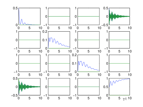
Figure 2: Time evolution of the density matrix elements for the parameters $\Delta_{1}=\Delta_{2}=2$, $\alpha_{1}=\alpha_{2}=2$, $\gamma=0.5$ and ${\overline{n}}=0$. The frequency $\omega_{1}$ is assumed to be $10$. The structure of the density matrix remains of the same form given in Eq. (62) for all parameters used in this paper.

IV Dynamics of entanglement quantified by concurrence

In this section we consider the dynamics of the entanglement of the bipartite system $1-2$ in the non-Markovian reservoir assuming the system density operator $\rho_{12}(t=0)$ to be in the state (24) initially. We take Wootters concurrence Wootters1 ; Wootters2 to quantify the amount of entanglement present in the subsystem $\rho_{12}(t)$. The concurrence of a bipartite, arbitrary density operator $\rho$ of two qubits is defined as

$${\cal{C}}(\rho)=\text{max}\left\{0,\lambda_{1}-\lambda_{2}-\lambda_{3}-\lambda_{4}\right\},$$ (57)

where the $\lambda_{i}$ are the square roots of the eigenvalues of $\rho\tilde{\rho}$ in descending order. Here $\tilde{\rho}$ is the result of applying the spin-flip operation to the complex conjugation or transpose of $\rho$:

$$\tilde{\rho}=(\sigma_{y}\otimes\sigma_{y})\rho^{\ast}(\sigma_{y}\otimes\sigma_{y}),$$ (58)

where the complex conjugation is taken in the standard computational basis. The concurrence is related to the entanglement of formation ${{E}}_{f}(\rho)$ by the following function Wootters1 ; Wootters2

$${{E}}_{f}(\rho)={\cal{E}}[{\cal{C}}(\rho)],$$ (59)

where,

$${\cal{E}}[{\cal{C}}(\rho)]=h\left[\frac{1+\sqrt{1-{\cal{C}}^{2}(\rho)}}{2}\right],$$ (60)

and

$$h(x)=-x\log_{2}x-(1-x)\log_{2}(1-x).$$ (61)

The structure of the density matrix of the two-atom system remains in the following form during the time-evolution

$$\rho_{12}(t)=\left[\begin{array}[]{cccc}a(t)&0&0&f(t)\\ 0&b(t)&0&0\\ 0&0&c(t)&0\\ f^{\ast}(t)&0&0&d(t)\end{array}\right],$$ (62)

where $a(t)+b(t)+c(t)+d(t)=1$. This property is a consequence of the special initial condition and the fact that the environment, regardless of whether it is Markovian or not, can not create coherence that was not present initially. The time evolution of the density matrix is shown in Fig. 2 for a certain set of parameters. This particular form of the density matrix (62) allows us to analytically express the concurrence as

$${\cal{C}}[\rho_{12}(t)]=2\text{max}\{0,|f(t)|-\sqrt{b(t)c(t)}\}.$$ (63)

In Figs. 3-6 we plot the evolution of the concurrence for different parameters of the non-Markovian bath. As a result of the memory effects the concurrence displays an oscillatory time dependence, especially when the coupling parameter $\alpha$ is strong. In the case of zero detuning, $\Delta=0$, the entanglement can vanish after a finite time even when the initial state of the two-atom system is a maximally entangled Bell state, as shown in Fig. 4. However, due to the memory inherent in the non-Markovian bath, the entanglement is partially restored. The two-atom system remembers its initial degree of entanglement to some extent, which leads to a revival of the entanglement. The collapse and revival of the entanglement displays a damped oscillatory behavior in time, whose frequency depends on the coupling parameter $\alpha$. Thus the coupling parameter $\alpha$ characterizes the memory ability of the reservoir to some extent. In case when the detuning $\Delta$ differs from zero, the entanglement does not completely vanish after a finite time, as displayed in Fig. 3. The detuning suppresses the decoherence and thus extends the decoherence time. This is because the mini-reservoir atoms ‘shield’ atoms $1$ and $2$ from the reservoir. When the damping rate $\gamma$ is of the same order or greater than the coupling parameter $\alpha$, the decay of the entanglement is damping oriented and oscillations do not appear, as seen in Fig. 5. However, the effect of the non-Markovian bath is still visible, as the concurrence displays a non-exponential decay in time, and the decoherence time is extended. The last plot Fig. 6 displays the concurrence in the Markovian limit, which is achieved when $\alpha/\gamma\to 0$ but $\alpha^{2}/\gamma$ remains finite Salo . In this case the Markovian time scale is given as Salo

$$\Gamma=\frac{1}{(2\overline{n}+1)^{2}}\frac{\alpha^{2}}{\gamma},$$ (64)

leading to an effective decoherence rate of $\Gamma=1/3$ for the parameters used in Fig. 6.

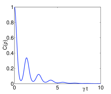
Figure 3: Evolution of the concurrence of an initially maximally entangled Bell state which decays into the non-Markovian reservoir. The dimensionless parameters of the reservoir are $\Delta_{1}=\Delta_{2}=2$, $\alpha_{1}=\alpha_{2}=2$, $\gamma=0.5$ and ${\overline{n}}=0$. The frequency $\omega_{1}$ is assumed to be $10$. The concurrence displays and oscillating behavior due to the memory effects of the non-Markovian reservoir. Entanglement which is initially lost due to decoherence is partially restored by the memory effects. Because of the large detuning, entanglement does not completely vanish in a finite time.

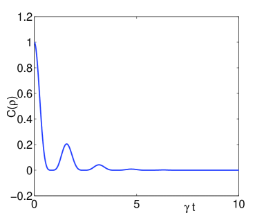
Figure 4: Evolution of the concurrence of an initially maximally entangled Bell state which decays into the non-Markovian reservoir. The dimensionless parameters of the reservoir are $\Delta_{1}=\Delta_{2}=0$, $\alpha_{1}=\alpha_{2}=2$, $\gamma=0.5$ and ${\overline{n}}=0$. The frequency $\omega_{1}$ is assumed to be $10$. As in Fig. 3 the concurrence displays and oscillating behavior due to the memory effects of the non-Markovian reservoir. However, the entanglement completely vanishes at finite times before it is partially recovered in contrast to Fig. 3. This is a consequence of the vanishing detuning.

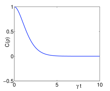
Figure 5: Evolution of the concurrence of an initially maximally entangled Bell state which decays into the non-Markovian reservoir. The dimensionless parameters of the reservoir are $\Delta_{1}=\Delta_{2}=0$, $\alpha_{1}=\alpha_{2}=0.5$, $\gamma=0.5$ and ${\overline{n}}=0$. The frequency $\omega_{1}$ is assumed to be $10$. The concurrence does not display an oscillating behavior any more since the interaction with the near environment is comparable weak and damping dominates. However, the decay of the concurrence is non-exponential which is a manifestation of the non-Markovian reservoir.

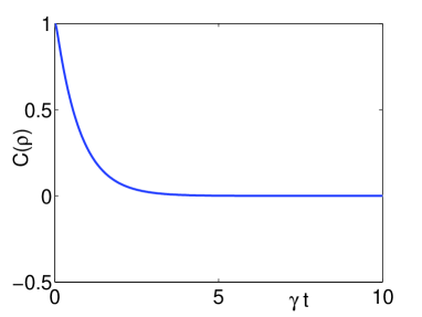
Figure 6: Evolution of the concurrence of an initially maximally entangled Bell state which decays into a Markovian reservoir which is achieved when $\alpha/\gamma\to 0$. The dimensionless parameters of the reservoir are $\Delta_{1}=\Delta_{2}=0$, $\alpha_{1}=\alpha_{2}=3$, $\gamma=27$ and ${\overline{n}}=0$ giving an effective Markovian decay rate of $\Gamma=1/3$ (see text). The frequency $\omega_{1}$ is assumed to be $10$.

An important observation with respect to entanglement is that for an open quantum system, entanglement can die off at finite times. It has recently been shown that this can happen not only when one starts with mixtures of entangled quantum states, but also in cases of initially pure and maximally entangled states, if the entangled system is coupled to a thermal reservoir at finite temperature Eberly1 ; Eberly2 ; Carvalho . In other words non-local disentanglement times are in general shorter than local decoherence times. In practical quantum computation schemes which operate at finite temperature this is of particular importance since some quantum computational algorithms rely on entanglement. We therefore ask next, to what extent a non-Markovian reservoir affects the decoherence of the entangled system in the case of an environment with non-zero temperature. This is illustrated in Figs. 7-11 for an environment with a mean photon number of $\overline{n}=0.2$, i.e. a hot reservoir.

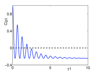
Figure 7: Evolution of the concurrence of an initially maximally entangled Bell state which decays into the non-Markovian reservoir of finite temperature with mean photon number $\overline{n}=0.2$. Here, we do not plot the actual concurrence but ${\cal{C}}[\rho_{12}(t)]=2\{|f|-[b(t)c(t)]^{1/2}\}$ instead of ${\cal{C}}[\rho_{12}(t)]=2\text{max}\{|f|-[b(t)c(t)]^{1/2}\}\geq 0$ to see how negative it becomes. The dimensionless parameters of the reservoir are $\Delta_{1}=\Delta_{2}=0$, $\alpha_{1}=\alpha_{2}=5$, $\gamma=1/3$ and ${\overline{n}}=0.2$. The frequency $\omega_{1}$ is assumed to be $10$. As in Figs. 3 and 4 the concurrence displays and oscillating behavior due to the memory effects of the non-Markovian reservoir. In contrast to the zero temperature case, however, the concurrence vanishes at a finite time completely and cannot be retrieved. In addition, during the time period where the concurrence can be partially recovered there are extended periods of time where it vanishes completely.

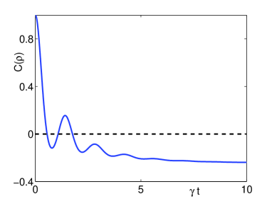
Figure 8: Same as Fig. 7 but with parameters $\Delta_{1}=\Delta_{2}=2$, $\alpha_{1}=\alpha_{2}=2$, $\gamma=0.5$ and ${\overline{n}}=0.2$. The frequency $\omega_{1}$ is assumed to be $10$.

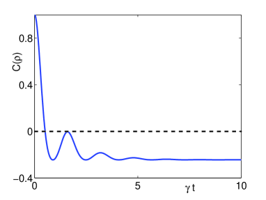
Figure 9: Same as Fig. 7 but with parameters $\Delta_{1}=\Delta_{2}=0$, $\alpha_{1}=\alpha_{2}=2$, $\gamma=0.5$ and ${\overline{n}}=0.2$. The frequency $\omega_{1}$ is assumed to be $10$.

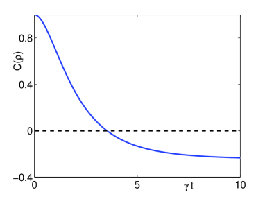
Figure 10: Same as Fig. 7 but with parameters $\Delta_{1}=\Delta_{2}=0$, $\alpha_{1}=\alpha_{2}=0.5$, $\gamma=1$ and ${\overline{n}}=0.2$. The frequency $\omega_{1}$ is assumed to be $10$. This figure displays the strong damping case in which the effect of the near environment is comparably weak. However non-Markovian effects are clearly visible since the decay of the concurrence is non-exponential. As a result the period of time during which the concurrence is maintained is extended compared to the Markovian decay.

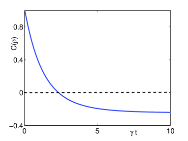
Figure 11: Evolution of the concurrence in the Markovian limit of the temperature reservoir. The parameters are $\Delta_{1}=\Delta_{2}=0$, $\alpha_{1}=\alpha_{2}=3$, $\gamma=27$ and ${\overline{n}}=0.2$ leading to an effective Markovian decay rate of $\Gamma\approx 1/6$. The frequency $\omega_{1}$ is assumed to be $10$. In comparison to Fig. 10 the concurrence is maintained during a shorter period of time.

In order to visualize the periods over which the concurrence becomes zero more clearly, we do not display the actual concurrence given in (63) but the quantity $2\{|f(t)|-[b(t)c(t)]^{1/2}\}$, which is less than zero when the concurrence vanishes. In contrast to the zero temperature case we can see that the concurrence vanishes suddenly after a finite time for all plots, a behavior which has been predicted for Markovian reservoirs in Eberly1 ; Eberly2 . In addition, in cases of strong coupling to the near environments, when $\alpha>\gamma$, the concurrence can vanish for a period of time, before being partially recovered due to the memory effect of the non-Markovian reservoir. As the interaction parameter $\alpha$ with the near environment becomes stronger, these periods of time when concurrence completely vanishes become shorter, and the rate at which the concurrence partially revives increases as shown in Figs. 7-9. The time until there is no more revival of the concurrence becomes longer when there is some detuning between the system under consideration and the near environment as can be seen by comparison of Figs. 8 and 9. When $\gamma>\alpha$ and the damping dominates, the effect of the non-Markovian reservoir becomes weaker and the evolution of the concurrence does not display an oscillating behavior any more. However the decay of the concurrence is non-exponential and the period of time before it vanishes completely can be extended in comparison with a Markovian reservoir, as can be seen by comparing Fig. 10 with Fig. 11, which shows the Markovian limit. For the parameters given in Fig. 11 the effective Markovian decay rate $\Gamma$ for the Markovian limit can be calculated from Eq. (64) to be $\Gamma\approx 1/6$. Although this effective decay rate is considerably smaller than the decay rate $\gamma=1$ used in the non-Markovian reservoir of Fig. 10, the period of time before the concurrence suddenly vanishes is shorter than for the non-Markovian reservoir. Thus a non-Markovian reservoir helps to maintain concurrence over a larger period of time in comparison to a Markovian reservoir.

V Summary and Conclusions

In this paper we have discussed the effects of a non-Markovian bath on the decoherence of an entangled two-atom system where the atoms are assumed to be two-level systems representing qubits. The non-Markovian bath is described by a model that leads to an exact Nakajima-Zwanzig type master equation that can be solved without any approximations, as discussed by Salo et al. in Salo . The advantage of this master equation is that it leads to a completely positive time evolution and therefore non-physical quantum states do not arise, a situation which can appear in parameterized phenomenological non-Markovian master equations Barnett1 .

We discuss the time-evolution of the entanglement of an initially maximally entangled Bell state in this non-Markovian reservoir. The entanglement is quantified by the concurrence Wootters1 ; Wootters2 which can be derived in an analytical form since the density matrix of the two-atom system retains a certain structure during time evolution. The dynamics of the concurrence displays some interesting features which are manifestations of the memory effects inherent in a non-Markovian reservoir. In particular, the entanglement can vanish after a finite time but, depending on the parameters of the reservoir, it can be partially restored. The revival of the concurrence is an effect that is specific to the non-Markovian reservoir since the reservoir remembers that the system was initially completely entangled, and some of this entanglement can be restored in the principle system even though it becomes zero during the time evolution.

In the case of finite temperature baths it is well known that the concurrence of an entangled system can experience “sudden death” when the system decays into a Markovian reservoir Eberly1 ; Eberly2 ; Carvalho . This sudden death of the concurrence can not be prevented in a thermal non-Markovian reservoir either. However, due to the memory effect in the non-Markovian reservoir the concurrence can revive even when it completely vanished after a finite period of time. Depending on the parameters used, the concurrence displays a collapse and revival structure in time, which finally ends in sudden death. The time of the sudden death can be extended by the non-Markovian reservoir in comparison with the Markovian reservoir. This is an effect of the non-exponential decay of the concurrence in a non-Markovian reservoir compared with its exponential decay in a Markovian reservoir.

References

• [1] H. P. Breuer and F. Petruccione, The Theory of Open Quantum Systems (Oxford University Press, Oxford, 2002).
• [2] G. S. Lindblad, Commun. Math. Phys. 48, 119 (1976).
• [3] V. Gorini, A. Kossakowski, and E. C. G. Sudarshan, J. Math. Phys. 17, 821 (1976).
• [4] F. Benatti, R. Floreanini, and R. Romano, J. Phys. A: Math. Gen. 35, L551 (2002).
• [5] R. Alicki, M. Horodecki, P. Horodecki, and R. Horodecki, Phys. Rev. A65, 062101 (2002).
• [6] R. Alicki, M. Horodecki, P. Horodecki, R. Horodecki, L. Jacak, and P. Machnikowski, Phys. Rev. A70, 010501(R) (2004).
• [7] D. Ahn, J. Lee, M. S. Kim, and S. W. Hwang, Phys. Rev. A66, 012302 (2002).
• [8] J. Lee, I. Kim, D. Ahn, H. McAneney, and M. S. Kim, Phys. Rev. A70, 024301 (2004).
• [9] S. Daffer, K. Wódkiewicz, J. D. Crasser, and J. K. McIver, Phys. Rev. A70, 010304(R) (2004).
• [10] B. M. Terhal and G. Burkard, Phys. Rev. A71, 012336 (2005).
• [11] P. Aliferis, D. Gottesman, and J. Preskill, Quant. Inf. Comput. 6, 97 (2006).
• [12] S. Nakajima, Prog. Theor. Phys. 20, 948 (1958).
• [13] R. Zwanzig, J. Chem. Phys. 33, 1338 (1960).
• [14] F. Shibata, Y. Takahashi, and N. Hashitsume, J. Stat. Phys. 17, 171 (1977).
• [15] S. M. Barnett and S. Stenholm, Phys. Rev. A64, 033808 (2001).
• [16] A. A. Budini, Phys. Rev. A69, 042107 (2004).
• [17] A. Shabani and D. A. Lidar, Phys. Rev. A71, 020101 (2005).
• [18] S. Maniscalco, Phys. Rev. A72, 024103 (2005).
• [19] S. Maniscalco and F. Petruccione, Phys. Rev. A73, 012111 (2006).
• [20] J. Salo, S. M. Barnett, and S. Stenholm, Opt. Commun. 259, 772 (2006).
• [21] W. K. Wootters, Phys. Rev. Lett. 80, 2245 (1998).
• [22] W. K. Wootters, Quant. Inf. Comp. 1, (1) 27 (2001).
• [23] T. Yu and J. H. Eberly, Phys. Rev. Lett. 93, 140404 (2004).
• [24] T. Yu and J. H. Eberly, quant-ph/0503089 (2005).
• [25] M. Jakob , Y. Abranyos, and J. A. Bergou, Phys. Rev. A64, 062102 (2001).
• [26] M. Jakob, Y. Abranyos, and J. A. Bergou, Phys. Rev. A66, 022113 (2002).
• [27] C. J. Myatt, B. E. King, Q. A. Turchette, C. A. Sackett, D. Kielpinski, W. M. Itano, C. Monroe, and D. J. Wineland, Nature (London) 403, 269 (2000).
• [28] Q. A. Turchette, C. J. Myatt, B. E. King, C. A. Sackett, D. Kielpinski, W. M. Itano, C. Monroe, and D. J. Wineland, Phys. Rev. A62, 053807 (2000).
• [29] S. M. Barnett and P. L. Knight, Phys. Rev. A33, 2444 (1986).
• [30] A. R. R. Carvalho, F. Mintert, S. Palzer, and A. Buchleitner, quant-ph/0508114 (2005).