Quantum Teleportation with Continuous Variables: a survey
Abstract
Very recently we have witnessed a new development of quantum information, the so-called continuous variable (CV) quantum information theory. Such a further development has been mainly due to the experimental and theoretical advantages offered by CV systems, i.e., quantum systems described by a set of observables, like position and momentum, which have a continuous spectrum of eigenvalues. According to this novel trend, quantum information protocols like quantum teleportation have been suitably extended to the CV framework. Here, we briefly review some mathematical tools relative to CV systems and we consequently develop the concepts of quantum entanglement and teleportation in the CV framework, by analogy with the qubit-based approach. Some connections between teleportation fidelity and entanglement properties of the underlying quantum channel are inspected. Next, we face the study of CV quantum teleportation networks where more users share a multipartite state and an arbitrary pair of them performs quantum teleportation. In this context, we show alternative protocols and we investigate the optimal strategy that maximizes the performance of the network.
pacs:
03.67.Hk, 03.67.Mn, 03.65.CaI Introduction
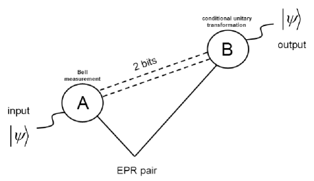
Ideally, quantum teleportation consists in the perfect transfer of an unknown quantum state from a sender, usually called Alice, to a remote receiver, usually called Bob TeleBennett . To accomplish this task, Alice divides the full information of into two parts, one classical and the other non-classical, and send them to Bob through two different channels: the classical channel and the quantum channel. The first one can be a telegraph wire, while the latter one is a bipartite quantum system with strong long-range correlations and which is distributed in advance between the two parties. After these transmissions, Bob can act on the quantum channel reconstructing a perfect replica of , while the original Alice’s state is destroyed during the process (as a direct consequence of the no-cloning theorem NoCloning ). The net result of the teleportation is the removal of from Alice’s side and its appearance in Bob’s side some time later, just the time needed by a classical message to go from Alice to Bob.
The depicted general protocol for quantum teleportation is based on a fundamental ingredient: the quantum channel which is shared by the two parties. It consists in a bipartite state of two distant systems and , possessed by Alice and Bob, respectively, and whose correlations are exploited to teleport the input state. This is possible by mixing the input state with the quantum channel at Alice’s side (system ) via a suitable collective measurement, called Bell measurement, whose projective effect causes the flow of quantum information to system via the long-range correlations. The result of the measurement is then sent to Bob through the classical channel, and Bob uses this additional classical information to completely retrieve the input state from his system . This is possible by performing a unitary transformation which is conditioned to the particular outcome of the Bell measurement.
Bennett et al. TeleBennett first show how the strong correlations between a pair of qubits and , prepared in the Einstein-Podolsky-Rosen (EPR) state
| (1) |
can assist the perfect teleportation of an unknown pure quantum state from Alice to Bob (see Fig. 1). The initial total state , involves no correlations between the unknown qubit and the EPR pair. In order transmit the information through the quantum channel, Alice couples the input qubit with the qubit of the EPR pair by performing a Bell measurement. This a joint measurement over the qubits and given by the projection on the orthonormal basis
| (2) | |||||
| (3) |
which is called Bell basis. Since the total state before the measurement can be expressed in terms of the Bell basis as
| (4) |
where
are the Pauli operators, it follows that the four outcomes of the Bell measurement have all the probabilities equal to , and after the measurement, the qubit will be projected into one of the following states
| (5) |
In every case, Bob’s qubit will be described by a state simply related to the original one . If now Alice communicates to Bob the exact outcome of her measurement, Bob can consequently apply the right unitary transformation on qubit which retrieves the original input state. This is the classical part of the protocol, i.e., the remaining information about the input state is represented by two bits of classical information which are produced by the measurement process. Exactly this amount of information has to be communicated from Alice to Bob through a classical channel in order to transmit the complete information about and therefore complete the teleportation process.
Ideally, using a quantum channel as the previous EPR pair would allow for a perfect quantum teleportation, where the output state is exactly equal to the input one. However, in any real situation, Alice and Bob access limited resources and the output state will be similar to input one by quantity called fidelity, which is defined as
| (6) |
where the bar denotes the average over many instances of the process (or the outcomes of the Bell measurement). In particular, for a pure input state , formula (6) simply becomes
| (7) |
One can ask if teleportation could be implemented classically, i.e., without any shared quantum resource. For instance, in a purely classical strategy, Alice can measure the input state on a fixed orthonormal basis and communicate the outcomes to Bob, who, in turn, tries to reconstruct the state from this classical information. However, Ref. Popescu proved that the purely classical channel can give at most , and therefore the region corresponds to a purely quantum teleportation.
In order to better understand this point, one has to introduce the concept of entanglement between two quantum systems. Basically, a bipartite quantum state is entangled when it cannot be reproduced via local operations and classical communication from the uncorrelated state Werner . Entanglement is a physical resource which can be quantified by introducing suitable entanglement measures HOROmono , and quantum teleportation is a process which exploits this resource. When a bipartite system has a high degree of entanglement, the correlations between its two subsystems and are so strong that they are not reproducible by any classical means. In other words, there is no local classical description (local hidden-variable theory) that can account for them, which are therefore purely quantum and descend directly from the non-locality behavior of quantum mechanics (marked by the violation of the Bell inequalities). Exactly exploiting such a kind of quantum correlations, it is possible to implement a purely quantum teleportation, not reproducible by any classical strategies. Ref. Horodecki5 proved that every two-qubit state which violates some generalized Bell inequality, (representing, therefore, a channel with non-local quantum correlations), allows to implement a teleportation with fidelity (i.e., purely quantum). Consider, for instance, the Werner mixture Werner
| (8) |
where is the identity operator, is the EPR state of Eq. (1), and is a parameter quantifying the entanglement relation . One can prove Peres that is entangled for , while the Bell inequality is violated in the narrower region . Here, non-local quantum correlations between the subsystem and enable to implement a purely quantum teleportation, i.e., with fidelity . In particular for , coincides with the EPR state which is a maximally entangled state and allows to perform an ideal quantum teleportation ().
All the previous considerations concerned the world of qubits, which are quantum systems described by a two-dimensional Hilbert space. In this paper, instead, we consider quantum systems described by a Hilbert space with infinite dimension. This is the case of the quantum oscillators or modes, which can be, e.g., the radiation modes of the electromagnetic field or the vibrating modes of a mechanical oscillator. Thanks to the infinite dimensionality of their Hilbert space, these systems can be described by observables, like position and momentum, which have a continuous spectrum of eigenvalues. When we use these continuous variables to characterize their state, we refer to these systems as continuous variable (CV) systems, and the usage of such variables in order to encode, process and transmit both classical and quantum information, gives rise to the CV quantum information and computation theory cvbook . In particular, we will review quantum teleportation for CV systems. In Sec. II we will introduce the necessary mathematical formalism to treat CV systems and Gaussian states. Then, in Sec. III we will treat quantum entanglement for CV systems, and in Sec. IV we will describe quantum teleportation in the CV framework together with its connection to CV quantum entanglement. In the subsequent Sec. V we will extend CV quantum teleportation from two to more users (CV quantum teleportation networks) and we will study possible protocols in the case of three parties. Finally, Sec. VI is for conclusion.
II Continuous variable systems and Gaussian states
Consider quantum oscillators labelled by , to which Hilbert spaces are associated. These modes are fully described by ladder operators satisfying the bosonic commutation relations and . Equivalently, they can be fully described by dimensionless conjugate quadratures Loock ; QOptics
| (9) |
satisfying the canonical commutation relations (CCR)
| (10) |
Introducing the vector of quadratures , the CCR be cast in the compact form
| (11) |
where
| (12) |
and denotes the direct sum. An arbitrary state of the modes is equivalently described by its symmetrically-ordered (or Wigner) characteristic function , where is the Weyl operator and . In particular, the state is said to be Gaussian if the corresponding characteristic function is Gaussian, i.e.,
| (13) |
In such a case, the state is fully characterized by its displacement , and its correlation matrix (CM) , whose generic element is defined as
| (14) |
where . All the information about the quantum and/or classical correlations among the oscillators is contained in the CM, which is a , real and symmetric matrix satisfying the bona fide condition
| (15) |
which corresponds to the uncertainty principle CCRcompact . By applying the Fourier transform to Eq. (13) one gets the Wigner function of the arbitrary Gaussian state which is again a Gaussian function and it is given by
| (16) |
In Eq. (16), the variables , conjugate of , are the continuous variables corresponding to the quadratures , and define the dimensional phase space of the system. These real variables can be arranged into complex amplitudes
| (17) |
and the Wigner function of Eq. (16) can be expressed in terms of the vector and denoted as .
Note that, since a Gaussian state of modes has a one-to-one correspondence with its first and second moments, it requires only real parameters for its full description, which is polynomial rather than exponential in IntroGauss . This mathematical tractability together with their experimental commonness have made Gaussian states the object of an intensive study during the last years.
II.1 Symplectic transformations
The most general real linear transformation over the quadratures ,
| (18) |
must preserve the CCR (11) in order to be a physical operation. This happens when the linear map (18) is described by a , real matrix [to be denoted as ], which satisfies the condition
| (19) |
The set of all matrices satisfying Eq. (19) forms the so-called real symplectic group , whose elements are called symplectic or canonical transformations. An arbitrary symplectic transformation (18) of the quadratures acts on the corresponding continuous variables of the phase space as . Therefore, it transforms the Wigner function as a scalar
| (20) |
and corresponds to a congruence at the level of the CM
| (21) |
Eq. (21) represents the relevant phase-space transformation when only the second moments are object of investigation. An arbitrary symplectic transformation acting on the phase space corresponds to a unitary operator acting on the Hilbert space , which transforms the state according to the law . The corresponding unitary operator can be determined via the relation
| (22) |
Those particular unitary operators defined by Eq. (22) are called linear unitary Bogoliubov operations (LUBOs) and, since they preserve the Gaussian character of a density matrix, they are also called Gaussian unitary transformations IntroGauss . Symplectic transformations of the form are local, and correspond to local linear unitary Bogoliubov operations (LLUBOs) having the form with acting only on .
Due to a theorem by Williamson Will , the CM of a mode Gaussian state can always be written as
| (23) |
where and
| (24) |
The quantities ’s in Eq. (24) represent the symplectic eigenvalues of the CM and they are clearly invariant under symplectic transformations. In the Hilbert space, the dual formulation of Eq. (23) reads
| (25) |
where is a thermal state Gardiner having a mean excitation number such that . The symplectic eigenvalues ’s encode essential information on the Gaussian state, and provide powerful ways to express its fundamental properties. For instance, the condition characterizes pure states, as it can be shown by the Von Neumann entropy which is equal to Holevo
| (26) |
where
| (27) |
In particular, the uncertainty principle of Eq. (15) can be cast in the following equivalent form
| (28) |
which is saturated only by pure Gaussian states.
Consider now the particular case of Gaussian states of only two modes. In this case, it is convenient to write the CM in the blockform
| (29) |
where and . For bipartite Gaussian states, the two symplectic eigenvalues of the CM are proved Alessio to be equal to
| (30) |
where
| (31) |
Here, the quantities and are invariant under (global) symplectic transformations. Furthermore, suitable local symplectic transformations allows to transform the CM of Eq. (29) into its normal form or standard form I SimonPRL
| (32) |
where and are four local symplectic invariants of the original CM.
III Continuous variable entanglement
III.1 Peres-Horodecki separability criterion for continuous variable systems
Consider two quantum systems labelled by letter (referring to Alice) and (referring to Bob), which correspond to two Hilbert spaces and , respectively. An arbitrary state of these two systems is called separable when it can be written as a convex sum of tensor products of single-party states Werner , i.e.,
| (33) |
with and . In such a case the bipartite state can be prepared via local operations and classical communications (LOCCs) acting on two uncorrelated subsystems and . On the contrary, is said entangled when Eq. (33) does not hold.
In the case of finite dimensional Hilbert spaces, i.e., and , a simple criterion to test separability was derived by Peres Peres who resorted to the so-called partial transpose (PT) operation. Introducing an orthonormal basis in the Hilbert space , the arbitrary state of the bipartite system is described by a density matrix , where Latin indices refer to the first subsystem () and Greek indices to the second one (). Now the PT operation can be defined as an inversion of the Greek indices
| (34) |
In Eq. (34) we ask if the operator is still a density operator, i.e., if and . Since the PT operation preserves the diagonal elements of the density matrix, the genuineness of the final state simply corresponds to its positivity. By definition, those density operators , for which holds, are called positive partial transpose (PPT) states. Peres showed Peres that the PPT property is a necessary condition for separability
| (35) |
and, in the particular case of two qubits, it is also sufficient
| (36) |
Later on, R. Simon SimonPRL showed how to extend the PT operation (34) and the Peres criterion (35-36) to the case of CV bipartite states, i.e., for bipartite states of two modes and . Let us introduce the phase space representation of a CV bipartite state via its Wigner function where . In phase space, transposition is defined as “time reversal” (or mirror reflection) which is given by a change of sign of momentum operators. Partial transposition is therefore a “local time reversal” which inverts the momentum of only one subsystem. Thus, the PT operation on the state in
| (37) |
is equivalent to the following partial mirror reflection of the Wigner function in phase space
| (38) |
where , with
| (39) |
and the identity matrix. Consequently, the CM of the state is transformed according to the law
| (40) |
For this reason, we can extend the Peres criterion (35) to CV bipartite states as
| (41) |
where bona fide means “corresponding to a physical state” and it is expressed by condition of Eq. (15) at the level of the second moments. Therefore, we can write the necessary condition
| (42) |
where the right-hand of Eq. (42) is also known as PPT property for the CM , by analogy with Eq. (35). More strongly, one can prove SimonPRL the following theorem in the case of Gaussian states
- Theorem.
-
Consider an arbitrary bipartite Gaussian state . Then
(43)
Note that, in the right hand of the previous Eq. (43), CM must also implicitly satisfy the bona-fide condition of Eq. (15). This remark is important when the entanglement properties are studied through the second moments and completely arbitrary CM’s are considered in the investigation, as, for instance, in deriving computable criteria for separability Commento .
The study of CV entanglement acquires an elegant form by resorting to the formalism of symplectic invariants. Consider an arbitrary Gaussian state whose CM is put in the blockform of Eq. (29). One can then verify that the PT transformation reduces to the sign flipping at the level of the local symplectic invariants. For this reason, the two symplectic eigenvalues of the partially transposed CM satisfy Eq. (30) except for the replacement
| (44) |
If we now apply Eq. (28) to the equivalence of Eq. (43), we can conclude the following
- Theorem.
-
Consider an arbitrary bipartite Gaussian state . Then
(45)
In general, one is able to provide not only a test for bipartite entanglement as before, but also computable measures of entanglement, called entanglement monotones VidMono , whose fundamental property is to be monotonic under LOCCs HOROmono . This is the case of the negativity and logarithmic negativity which are defined for discrete variable states and suitably extended to Gaussian states of CV systems VidalW . Consider an arbitrary bipartite state of a system, its negativity is defined as
| (46) |
where is the trace norm (Schatten 1-norm). One can verify that is equal to the modulus of the sum of the negative eigenvalues of . In this sense, the negativity quantifies the extent to which fails to be positive and, intuitively, represents a measure of the bipartite entanglement within . Similarly, the logarithmic negativity is defined as and has the remarkable property to be additive under tensor product. These measures can be readily extended to bipartite Gaussian states by interpreting the PT operation as partial mirror reflection as before. In such a case, one can prove Salerno1 that
| (47) |
where is the minimum PT-symplectic eigenvalue of . Thanks to its monotonic relation with the logarithmic negativity, the minimum PT-symplectic eigenvalue can be adopted as entanglement monotone for bipartite Gaussian states.
III.2 Bipartite entanglement and EPR correlations
Besides R. Simon, also L.-M. Duan et al. DuanPRL derived a criterion for entanglement, which turns out to be very useful for teleportation. As usual, consider two modes, and , with quadrature operators and . From these operators, we can define the following EPR-like operators
| (48) |
where . Note that for we have the standard EPR operators
| (49) |
An arbitrary state of the two-mode system satisfies the following necessary condition for separability
| (50) |
where and denote the variances of and , computed over the state . From (50) one derives the following sufficient criterion for entanglement
- Criterion.
-
If such that
(51) then is entangled.
As we have already said, a bipartite Gaussian state can be fully described by its displacement and CM. Since its separability properties do not vary under unitary operations, we may cancel its displacement via local displacement operators, and reduce its CM to the normal form of Eq. (32) via a sequence of local symplectic transformations (local squeezings and rotations). The final state has the same separability properties of the original one, but it is associated to a simpler pair and. Consider now those states having a CM of the type whose peculiarity is to satisfy the equality
| (52) |
For these states, one can use the quantity as a measure of the correlations between the position and momentum observables of modes and . In fact, here, quantifies the two-mode squeezing in both the EPR operators and . For we say, by definition, that the two modes possess EPR correlations in and , and the corresponding state is an EPR channel. Note that implies that is an entangled state (from Eq. (51) with ). But if one cannot exclude the existence of another pair of EPR-like operators and which implies entanglement according to Eq. (51). Thus, entanglement is only a necessary condition for the existence of EPR correlations for a particular pair of conjugate quadratures. If we take the limit in Eq. (52), we achieve the perfect EPR correlations
| (53) |
i.e., we achieve the ideal EPR state EPR . This state represents the CV version of the discrete EPR pair of Eq. (1). It is a maximally entangled state () and, as we shall see, it allows to perform an ideal quantum teleportation.
Consider now the two-mode squeezed vacuum (TMSV) state or twin beam (TB) state, which is a bipartite Gaussian state having Wigner function
| (54) |
where the CM
| (55) |
depends on a squeezing factor . Note that the CM of Eq. (55) is a particular CM of the type , showing that the twin beam is an example of EPR channel. One can easily verify that which shows that, for every , one effectively has corresponding to two-mode squeezing, i.e., EPR correlations. If we now take the limit of infinite squeezing in Eq. (54), we achieve
| (56) |
i.e., we obtain the ideal EPR state EPR . As we shall see, this asymptotic state enables to implement a perfect CV quantum teleportation. However, in any real experimental setup, one can only access finite squeezing, and, therefore, exploit quantum channels as the TMSV state of Eq. (54).
IV Continuous variable quantum teleportation
Thanks to the elements developed in the previous sections, we are now ready to discuss quantum teleportation within the continuous variable framework. First of all, one can ask why the need of a CV quantum teleportation, since the discrete one already exists. Some important facts can be quoted to justify this further development of teleportation and they are mainly connected with experimental advantages. In fact, one of the key-points of the discrete variable protocol is the usage of a Bell measurement in order to couple the input qubit with the quantum channel. Till now, in all the real experimental setups, such a measurement has not been implemented in a clear and precise way. In other words, the perfect Bell-state discrimination does not seem to be achievable in a simple way, e.g., by linear passive elements as beam splitters and photodetectors BellB0 . On the contrary, the CV version of the Bell measurement is realized via linear passive optics and homodyne measurements, whose outcomes can be discriminated with high precision (perfectly discriminated in asymptotic sense).
Essentially, CV quantum teleportation is based on the same ideas of the discrete case. The basic resource is always the same, i.e., (CV) entanglement shared between Alice and Bob, which is a necessary condition in order to have a pair of (CV) EPR-correlated observables to be exploited in the protocol by the two parties. For sufficiently high entanglement, quantum channel reveals non-local quantum correlations that enable to perform a truly quantum teleportation, i.e., a teleportation process with fidelity , where is the fidelity of the best classical strategy. In the CV case, for arbitrary input states (instead of , as for the qubits), while, for the particular task of teleporting coherent states, one has F1su2 . Such a threshold has been proved to be connected with the violation of a CHSH inequality in Ref. ClassicF .
The protocol can be shown by analogy with the one for qubits. As usual, Alice mixes the unknown input state with the shared quantum channel via a Bell measurement, which, in continuous variables, is realized by a beam splitter and two homodyne detectors. In this way she sends part of information on the state to Bob via the quantum channel. In order to complete the process, Bob needs also to know the result of Alice’s measurement and this is exactly the part of classical information on the state that Alice communicates to Bob through the classical channel (this classical information is equal to two bits in the discrete case, while it is given by two real variables in the CV case). Conditioned to this classical information, Bob performs a suitable unitary operation on his part of quantum channel (which is a Pauli operator in the discrete case, while it is a displacement operator in CV) and correctly reconstructs the original input state that was in Alice’s hands. The net result of the teleportation is the removal of the input state from Alice’s side and its appearance in Bob’s side some time later (the time needed by a classical message to go from Alice to Bob).
In the following we will first present the ideal situation of a perfect CV quantum teleportation, which one has in the case of an ideal EPR pair as quantum channel. Such analysis will be carried out in the Heisenberg picture for its simplicity. Then, we will switch to a more real situation, where the quantum channel is imperfect (given by an arbitrary two-mode state), and this subsequent analysis will be carried out in the Schroedinger picture and using the Wigner representation in phase space.
IV.1 Ideal CV quantum teleportation
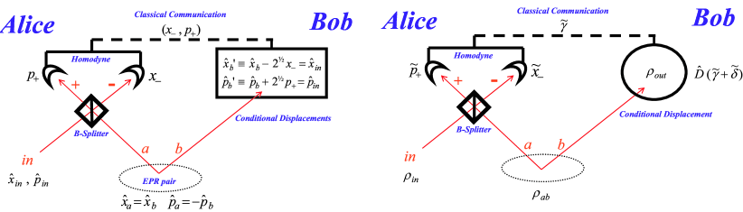
The proposal for a CV quantum teleportation was firstly made by Vaidman in Ref. vaidman and then by Braunstein and Kimble in Ref. KimbleTele . The ideal situation of a quantum channel given by an ideal EPR pair can be easily shown in the Heisenberg picture. The protocol goes as follows (see also Fig. 2, left side):
-
1.
Initial condition. Alice and Bob share a quantum channel given by an ideal EPR pair, i.e., two modes and with quadratures such that
(57) Then, Alice has an unknown input state described by an input mode with quadratures .
-
2.
Bell measurement. Alice realizes a CV version of the Bell measurement combining two subsequent operations on her modes
-
(a)
Beam splitter mixing. Alice mixes the input mode with her mode (part of the EPR pair) via a balanced (lossless) beam splitter, i.e., she performs the following bilinear transformation on their quadratures
(58) where and are the quadratures of the output modes “” and “” of the beam splitter.
-
(b)
Homodyne detection. Alice homodynes the output modes “”. In particular, she detects the quadratures and , i.e., she applies the projectors to mode “” and to mode “” notaEPR . Denoting with the two outcomes, her measurement causes in Eq. (58) the collapse
(59) Due to the EPR property (57), Bob’s quadratures, and , are instantaneously projected according to (59), i.e., we have
(60)
-
(a)
-
3.
Classical communication. At this point, Alice communicates her measurement result to Bob through a classical channel.
-
4.
Conditional displacement. Bob uses this transmitted classical information to perform a suitable conditional displacement on his own mode which allows to complete the teleportation process
(61)
In fact, according to Eq. (61), mode is finally described by a pair of conjugate quadratures ( and ) which are exactly the ones of the input ( and ). In the Schroedinger picture, this is equivalent to teleport the quantum state from the input mode , at Alice’s side, to the output mode , at Bob’s side, with fidelity .
IV.2 Real CV quantum teleportation
As we have already said in the introduction of Sec. IV, the previous situation, based on an ideal EPR pair, can only be considered as a limit of infinite squeezing of a real teleportation process, where the quantum channel has a finite amount of squeezing. Actually, also the homodyne measurement cannot be infinitely precise, and this detection inefficiency can be explicitly taken into account DABELL . Here, we will ignore this measurement imperfection and we will focus our attention on the more fundamental point concerning the reality of the channel. In particular, our analysis is carried out for quantum channels given by two-mode Gaussian states.
In this section we first show CV quantum teleportation through an arbitrary two-mode state, adopting the Schroedinger picture and, in particular, the phase space Wigner representation Chiz ; FIU ; JMO . We repeat the previous four-step analysis of the protocol in this general situation and using this different formalism Chiz . Then, we will consider the case of a Gaussian two-mode state, and we will obtain a very simple and useful formula for the fidelity FIU ; JMO . Such a case comprises the Gaussian EPR channel (see Sec. 51) and, in particular, the TMSV which is the real analog of the ideal EPR pair. The protocol goes as follows (see also Fig. 2, right side):
-
1.
Initial condition. Alice and Bob share a quantum channel given by an arbitrary state of two modes and . Such a state can be fully characterized by its Wigner function , where the complex amplitudes and refer to mode and , respectively. Then, Alice has an unknown input state of a single mode , whose complex amplitude is and Wigner function . The total initial state is given by the tensor product , and therefore it is described by the product
(62) -
2.
Bell measurement. Alice realizes a CV version of the Bell measurement combining two subsequent operations on her modes
-
(a)
Beam splitter mixing. Alice mixes the input mode with her mode via a balanced (lossless) beam splitter, i.e., she performs the following bilinear transformation on the complex amplitudes
(63) where are the complex amplitudes of the output modes . The total state just after the beam splitter is given by
(64) which is derived from Eq. (62) by using the inverse transformations of Eq. (63).
-
(b)
Homodyne detection. Alice detects the two quadratures and , and the corresponding outcomes can be expressed by a single complex number
(65) having probability . Due to her measurement, Alice remotely creates at Bob’s station (mode ) a conditioned state whose Wigner function is equal to
(66)
-
(a)
-
3.
Classical communication. Alice communicates her measurement result to Bob through a classical channel. After that Bob has received this classical information, the state of his mode is described by the Wigner function of Eq. (66).
-
4.
Conditional displacement. Bob uses the received classical information to perform a suitable conditional displacement on his own mode which aims to complete the teleportation process. What is now the “right” displacement? For a zero-displaced two-mode state, like the EPR pair of Eq. (57), the right displacement is given by Eq. (61), which is equivalent to the displacement
(67) The quantity in Eq. (67) is an extra-shift with respect to the original input state which is naturally generated by the process and, in particular, by the Bell measurement. In general, for a quantum channel given by a two-mode state with a nonzero displacement, Bob’s displacement must be composed by two terms. Besides , accounting for detection, there is another complex number which balances the shift inherited by the channel. Thus, the correct displacement has the form
(68) where depends on the first moments of the channel.
Notice that the displacement (68) is equivalent to set into the Wigner function (66) and consider the new variable . But, in order to simplify the notation, we can put and, therefore, the displacement (68) is equivalent to the formal substitution into Eq. (66). According to the previous four-step protocol, the final state at Bob’s station is given by
| (69) |
We may ask how much, on average, it is similar to the input state. In order to get teleportation fidelity , we compute the mean state teleported to Bob by averaging over all possible results
| (70) |
Inserting Eq. (69) into Eq. (70), we get the input-output relation
| (71) |
where the kernel
| (72) |
takes both the quantum channel and Bob’s additional displacement into account. If we now consider a pure state as input, the fidelity (7) takes the form
| (73) |
and, by using the input-output relation (71), we get the final formula
| (74) |
which expresses the fidelity as function of the input state, the channel and Bob’s additional displacement.
Let us consider the particular case of Gaussian states, i.e., a pure Gaussian state as input and a two-mode Gaussian state as channel. Such states are characterized by the two pairs and , respectively. From Eq. (74) one can prove that fidelity does not depend on the input displacement and, therefore, it will depend on the input and the channel via and , only. If we write in the blockform of Eq. (29) and , from Eq. (74) we get
| (75) |
where
| (76) |
and
| (77) | ||||
| (78) |
From Eq. (76) one can verify that the matrix is equal to
| (79) |
where and are the EPR operators. Thus, one can easily prove that and , so that in Eq. (77), and in Eq. (75). Matrix depends on CMs via Eq. (76), while the positive term is linked to vector via Eq. (77), which, in turn, contains both the shift of the channel and Bob’s additional displacement (see Eq. (78)) Without such a displacement (i.e., ), teleported state acquires a nonzero shift from the channel and the corresponding fidelity will depend upon such a shift via a decreasing exponential. In general, Bob can eliminate this shift by choosing an additional displacement which perfectly cancels the effects of according to Eq. (78), i.e.,
| (80) |
In such a case, fidelity of Eq. (75) becomes
| (81) |
i.e., it becomes independent from the displacement of the channel and it takes the maximum value, which is determined only by CMs and via the matrix . Thus, for a channel and an input state which are Gaussian, the “right” displacement at Bob’s station is given by Eq. (68) with given in Eq. (80), and the corresponding expression for the fidelity depends on the CMs of the channel and the input via the very simple Eq. (81).
IV.2.1 Fidelity, EPR correlations and entanglement
Suppose now that our quantum channel is a Gaussian two-mode state with CM in the normal form (32), i.e., and the input state is a coherent state, i.e., . Computing the matrix as in Eq. (76) and inserting the result into Eq. (81), the optimal fidelity turns out to be
| (82) |
where and . In particular, if then and , so that , i.e., teleportation is not quantum. On the contrary, if , i.e., , then we have as in Eq. (52), where quantity represents a measure of the EPR correlations of the relevant quadratures of the channel. From Eq. (82) it follows that
| (83) |
which shows that (for the considered class of channels) the existence of EPR correlations is equivalent to quantum teleportation, i.e.,
| (84) |
A Gaussian state described by a CM with represents a Gaussian EPR channel (see Sec. 51) and generalizes the two-parameter EPR channel studied in Ref. ClassicF . For this kind of channel, one can simply prove
| (85) |
But implication (85) holds in general for every quantum channel F1su2 . In fact, a teleportation protocol fully based on classical strategies is exactly a teleportation process which does not use any quantum entanglement between Alice and Bob, and since it implies a fidelity for coherent states’ teleportation, the condition is sufficient for the existence of bipartite quantum entanglement.
An important one-parameter Gaussian EPR channel is the TMSV state, with the squeezing-dependent CM specified in Eq. (55). In such a case , and therefore
| (86) |
which gives for while for . In this limit of infinite squeezing, the TMSV state becomes an ideal EPR pair and allows to implement a perfect quantum teleportation. In real experiments one can access only finite squeezing () and realize a quantum teleportation with fidelity like, e.g., in Ref. Furusawa , where the experimental value has been reported.
In general, it is an open problem to connect the entanglement of the quantum channel, shared by two parties, with the fidelity of teleportation of coherent states. In particular, one would like to show a monotonic relation between the fidelity and an entanglement monotone, like, e.g., the log-negativity or the minimum PT symplectic eigenvalue. Recently, Ref. AdessoTele showed that this is possible in the case of a thermal TMSV state, which can be described by the CM
| (87) |
where and are thermal noises which enters the system via modes and . Alice and Bob can try to fully exploit the resources of this channel by performing suitable LOCCs just before teleportation. For instance, they can apply local squeezing transformations, described in phase space by where . These local symplectic transformations do not alter the entanglement, i.e., the minimum PT symplectic eigenvalue remains unchanged from to , while the fidelity , computed via Eqs. (76) and (81), will depend on the parameter . One can then prove AdessoTele that takes a maximum for , for which we have
| (88) |
Thus, if Alice and Bob share a thermal TMSV state, the maximal teleportation fidelity for coherent states, achieved by optimizing over local squeezing transformations, is connected to the entanglement of the underlying quantum channel by the simple Eq. (88), which shows that is an entanglement monotone for this particular class of states.
V Continuous variable quantum teleportation networks
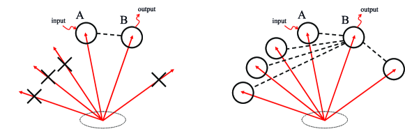
In the previous sections, we have recognized quantum entanglement as an important resource for quantum information purposes. In particular, bipartite entanglement represents the fundamental requirement that a shared quantum channel should have in order to enable a truly quantum teleportation. The possibility to generate multipartite entanglement, i.e., entanglement shared by more than two parties cinjap ; Lance ; FuruNat , has recently opened up the possibility to construct quantum teleportation networks. Here, a set of nodes have in common a quantum channel which enables to perform quantum teleportation between an arbitrary pair in the net. In a first strategy, the teleportation between these two arbitrary nodes can be implemented in the standard way (see Fig. 3), which corresponds to ignore all the other nodes and exploit the residual bipartite entanglement together with classical communications. This strategy is a direct extension of the standard teleportation protocol from two to more stations and we call it non-assisted protocol. But a more clever strategy is based upon a cooperative behavior, where all the other nodes assist the teleportation between the chosen pair (Alice and Bob) by means of LOCCs. In fact, if the external nodes perform suitable local measurements and then classically communicate their outcomes to Bob, the latter can use this additional classical information to improve the process via modified conditional displacements. We call this strategy assisted protocol.
In the CV domain, the idea of a CV quantum teleportation network was firstly developed in Ref. BraNetwork , where an easy way to produce CV multipartite entanglement was shown. The recipe of Ref. BraNetwork to create multipartite entanglement relies on a suitable distribution of squeezing. In the case of a single mode, a squeezed state is determined by two parameters: the complex amplitude and the complex squeeze factor , which is, in turn, composed by a real squeeze factor and a squeeze phase . Such a state can be generated by squeezing the vacuum and then by displacing it, i.e., where
| (89) |
is the one-mode squeezing operator, and
| (90) |
is the displacement operator (which expresses the Weyl operator in terms of complex amplitude). When two squeezed states are taken as input to a beam splitter, the squeezing mixes between the two modes and creates EPR correlations among their quadratures. For this reason, the state of the two output modes is entangled and such a procedure can be suitably extended from two to modes.
Let us consider a set of modes which will be then distributed to different nodes of a teleportation network. Before distribution, one can create a multipartite entangled state by applying local squeezing transformations to these modes, followed by a collective N-splitter transformation Nsplitter , which is a suitable sequence of beam splitter transformations. Denote by the initial vacuum state of the arbitrary mode (), and define the N-splitter transformation as
| (91) |
where
| (92) |
corresponds to a lossless beam splitter operation on the pair of modes and . Then, we can generate the following multipartite state
| (93) |
which is constructed by squeezing mode in momentum and the other modes in position, and then by applying the N-splitter (91) to all of them. The final state (93) is a Gaussian state with Wigner function cvbook
| (94) |
where and as usual. The multipartite state (94) is totally symmetric under interchange of nodes, so that every pair of them, among the different choices in the network, has the same resources for quantum teleportation. One can prove cvbook that the state (94) implies bipartite entanglement for every pair of the net, when all the other nodes are traced out. For this reason, it is a good quantum channel which, potentially, enables to perform quantum teleportation between an arbitrary pair of the net. It is straightforward to prove that, for , the Wigner function (94) is equal to the Wigner function (54) of the TMSV state, where the input squeezings (parameters and in Eq. (93) for ) are directly transformed in two-mode squeezing/EPR correlations (parameter in Eq. (55)). Practically, the state of Eq. (93), corresponding to the Wigner function of Eq. (94), represents the multi-mode version of the TMSV state, which we call N-mode squeezed vacuum (NMSV) state. Furthermore, if we take the limit of infinite squeezing in Eq. (94), such Wigner function becomes infinitely peaked at and (for ), i.e., it becomes the multi-mode version of the EPR state of Eq. (56)
| (95) |
This ideal N-mode EPR state can be rigorously defined as the zero-value eigenstate of the total momentum and relative positions . In the Heisenberg picture, it corresponds to the following conditions for the quadratures
| (96) |
The usage of an ideal N-mode EPR state, as shared quantum channel within a N-node CV quantum teleportation network (N-mode teleportation network, in the following), represents the ideal asymptotic situation corresponding to infinite squeezing, where one can exploit the perfect EPR correlations and perform perfect quantum teleportations within the network. But, actually, one can access only finite squeezing and, therefore, one can only exploit a multipartite channel as the NMSV state of Eq. (93) that has a finite amount of squeezing . In this real situation the performances of the teleportation processes are clearly lower.
In the following we will first present the case of an ideal CV quantum teleportation within the network, adopting the Heisenberg picture for simplicity. In particular, we will discuss two different protocols: the non-assisted protocol, which is connected to the notion of telecloning, and the assisted protocol, which exploits homodyne detection in the ideal case. Then, we will deal with a more realistic situation, where the quantum channel has not perfect EPR correlations. In such a case, teleportation fidelity is not equal to one, and it is open issue to determine what are the LOCCs that optimize the fidelity of the assisted protocol. This is the central problem analyzed in the subsequent sections. From now on, for simplicity, we consider only the case .
V.1 Ideal three-mode teleportation network
In the ideal three-mode teleportation network the quantum channel is given by an ideal 3-mode EPR state. Teleportation can be performed by two arbitrarily chosen nodes of the net, the sender (Alice) and the receiver (Bob), and the protocol can be assisted or non-assisted by the third node (Charlie). In the first case, a suitable homodyne detection of the third node allows to achieve a perfect teleportation (), while this is not possible in the latter case, due to the unexploited quantum resources owned by the third node. In this case, the third node may attempt to use his part of quantum channel to perform an additional teleportation from the sender to him (telecloning). In the Heisenberg picture we have the following protocol(s):
-
1.
Initial condition. Three distant parties, identified with Alice, Bob and Charlie, possess three different modes and , respectively, which have been prepared in the ideal 3-mode EPR state
(97) These three parties compose an ideal three-mode teleportation network since they can exploit their shared perfect EPR correlations (97) to implement an instance of perfect teleportation within the network. Suppose that one of the three, say Alice, wants to teleport to one of the other two, say Bob, an unknown state of an input mode with quadratures and .
-
2.
Bell measurement. Alice realizes the CV version of the Bell measurement on her modes by the usual two steps:
-
(a)
Beam splitter mixing. Alice mixes the mode with her mode (part of the channel) via a balanced beam splitter
(98) where and are the quadratures of the output modes .
-
(b)
Homodyne detection. Alice detects quadratures and . Denoting with the outcomes, her measurement causes in Eq. (98) the usual collapse
(99) Due to the EPR property (97), Bob and Charlie’s quadratures are instantaneously projected according to (99), i.e., we have
(100) (101) As we can see from Eq. (100), Bob’s momentum contains now an additional momentum operator with respect to Eq. (60). The presence of such an operator hints that Charlie can take an active part into the process and, at this point of the protocol, we may distinguish between assisted protocol and non-assisted protocol.
-
(a)
-
•
Non-assisted protocol. Charlie does not intervene in the process. Consequently, Alice and Bob ignores Charlie, and accomplish the teleportation according to the standard protocol shown in Sec. IV.1:
-
3
Classical communication. Alice communicates her measurement result to Bob through the classical channel.
-
4
Conditional displacement. Bob uses this classical information to perform the usual conditional displacement
(102) Contrary to Eq. (61), in Eq. (102) Bob does not obtain exactly the input momentum . In the Schroedinger picture, it means that the output state is not exactly the input one, but it has a certain fidelity because of the quantum resources owned by Charlie. What is the value of this fidelity? In order to answer to this question, assume that Alice has broadcasted her measurement result . In such a case, also Charlie receives this classical information and can attempt to teleport Alice’s input state to himself. From Eq. (101), we see that the best local operation he can do is the same of Bob, i.e., the conditional displacement
(103) Thus, independently and via the same shared quantum channel, both Bob and Charlie perform an imperfect teleportation from Alice. At the end of the whole process, the input state at Alice’s station is disappeared, and two imperfect copies appear at Bob and Charlie’s stations. On average (i.e., repeating the process many times with the same input) such copies are identical, but they cannot be identical to the original input state because of the no-cloning theorem NoCloning . For this reason, both the Alice-Bob and the Alice-Charlie teleportations have the same fidelity which must satisfy the bound , where is the optimal cloning fidelity for the states considered in input (for instance for coherent states NoCloCohe ). The whole protocol, where Bob and Charlie do not assist each other and perform two independent teleportations from Alice, represents the standard example of telecloning protocol CVteleCLO . In general, for telecloning we mean a process where an unknown input state is attempted to be teleported to different recipients so that (imperfect) clones are created at the remote locations.
-
•
(Ideal) assisted protocol. Charlie gets involved in the process with the aim of helping Bob. According to Eq. (100), the best thing he can do is to measure momentum and communicate the result . In fact, this additional information, besides the one communicated by Alice, allows Bob to perform a modified conditional displacement on his mode which establishes, again, at the output. In detail the assisted protocol goes as follows:
-
3’
Assisting measurement. Charlie performs a homodyne detection on his mode which realizes the measurement of the momentum . Denoting by the outcome, from Eq. (100) it follows the collapse
(104) -
4’
Classical communication. Alice and Charlie communicate their measurement results, and , to Bob through a classical channel.
-
5’
Conditional displacement. Bob uses the total classical information to perform a modified conditional displacement on his own mode
(105) which allows to complete the teleportation process. In fact, according to Eq. (105), mode is finally described by the conjugate quadratures of the input. In the Schroedinger picture this is equivalent to have teleported the state from Alice to Bob with fidelity .
V.2 Real three-mode teleportation networks
In the previous section, we have considered an ideal three-mode teleportation network, as generated by an ideal three-mode EPR state. Actually, in any real experimental setup, one can produce only finite squeezing and, therefore, imperfect EPR correlations. The corresponding real quantum channels imply teleportation processes with lower performances, i.e., with , even if it can be very close to one. Remarkable examples of real quantum channels are the 3MSV state, i.e., the NMSV state (93) with , and the following cheap three-mode state
| (106) |
which is generated by squeezing only one mode before the 3-splitter. The latter channel is sufficient to allow quantum teleportation between every pair of nodes in the net since, for every , it gives for teleportation of coherent states, if the assisted protocol is adopted BraNetwork . In addition to these quantum channels realized using squeezers and beam splitters, there are other examples of three-mode quantum channels, as the ones generated by inter-linked bilinear interactions Paris or by radiation pressure within opto-mechanical systems PRL ; PRAtele . Also in these cases quantum teleportation within the networks have been proved to be feasible and an assisted strategy, consisting in a LOCC by Charlie, can be proved to improve the process. It must be stressed that such a LOCC must not be necessarily based upon a homodyne detection at Charlie’s site, as it happens in the ideal case (and also in the case of the cheap state (106) and the 3MSV state). In general, when we consider general kinds of channels, there is the non trivial open question to determine what is the best LOCC that Charlie must perform, in order to optimize teleportation fidelity of the assisted protocol. Actually, such question is very general, and we will specialize it to the case of LOCCs given by local measurements at Charlie’s site. Then we will consider only the Gaussian case, i.e., shared quantum channels and input states which are Gaussian states. In detail, the open problem which we want to solve is
-
Problem
In a three-mode network where the quantum channel is given by an arbitrary three-mode Gaussian state, what is Charlie’s local measurement (and classical communication) which optimizes the fidelity of teleportation of pure Gaussian states between Alice and Bob?
In the following section we attempt to solve this problem of the assisted protocol. From a mathematical point of view, we can face the problem exploiting connections with the derivation of Sec. IV.2. Let us denote by the three-mode Gaussian state shared by Alice, Bob and Charlie. The non-assisted protocol is equivalent to trace Charlie and apply the above derivation to the two-mode reduced state , i.e., assuming as quantum channel between Alice and Bob. The assisted protocol, where Charlie performs a local measurement and communicates the result to Bob, can be treated by adopting that derivation with , where is the two-mode conditional state created by Charlie’s measurement.
V.3 Optimal local measurement
Consider a three-mode network where Alice, Bob and Charlie share a quantum channel given by a three-mode Gaussian state (three-mode Gaussian network from now on). Such quantum channel is used to perform quantum teleportation of a pure Gaussian state between two of the parties (Alice and Bob), while the third party (Charlie) can condition the process by means of LOCCs. Here, we show the best measurement that Charlie can perform on his own mode that preserves the Gaussian character of the three-mode state and optimizes the teleportation fidelity between Alice and Bob POVMpra . In other words, we find the optimal Gaussian measurement at Charlie’s site which maximizes the teleportation fidelity of the assisted protocol. Motivated by related results, we conjecture that this optimal Gaussian measurement is also the best among all possible measurements, trying to give a general answer to the problem of Sec. V.2. In Sec. V.3.1 we present the scenario and describe the teleportation protocols, assisted and not assisted by measurements at Charlie’s site. In Sec. V.3.2 we discuss the case when Charlie performs a dichotomic measurement with a Gaussian and a non-Gaussian outcome, while in Sec. V.3.3 we consider the case of a local Gaussian measurement. For simplicity, we have omitted the proofs of the theorems which are reported in Ref. POVMpra .
V.3.1 Assisted and non-assisted teleportation protocols
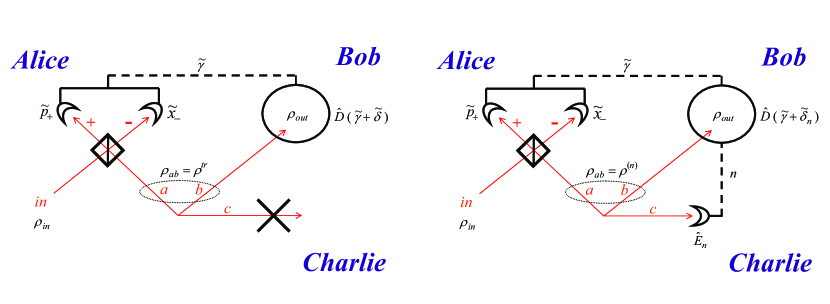
Let us consider a three-mode Gaussian network where Alice has to teleport an unknown pure Gaussian state to Bob. In a first strategy, Charlie is neglected, and Alice and Bob implement the standard CV teleportation protocol of Sec. IV.2 (non-assisted protocol). In an alternative strategy, Charlie performs a local measurement and classically communicates the result to Bob, who exploits this additional information in the teleportation process (assisted protocol). Here, we show the two protocols in detail (see also Fig. 4). For both protocols, the various steps are basically the same as presented in Sec. V.1, but, here, we prefer to show them giving the precedence to Charlie’s action (nothing in the first case, a LOCC in the second case). The inversion of the order between Alice and Charlie’s physical actions is possible because of the local character of their measurements, and it allows to study the process applying directly the results of Sec. IV.2.
-
1.
Initial condition. Alice, Bob and Charlie possess three different modes, characterized by annihilation operators and respectively, which are described by a three-mode Gaussian state , having displacement and CM
(107) where the blocks are real matrices. Alice has to teleport to Bob a single-mode pure Gaussian state with CM and displacement completely unknown to her. Since a single-mode pure Gaussian state is a single-mode squeezed state, we can put .
-
•
Non-assisted protocol. The most straightforward strategy is to ignore Charlie (see Fig. 4, left side) and use the reduced two-mode state to implement a standard CV teleportation protocol. It is easy to prove that such a state is a Gaussian state with CM
(108) and displacement . Thus, we can apply the results of Sec. IV.2, relative to Gaussian states, by taking .
-
2.
Bell measurement. Alice mixes her part of the channel (mode ) with the input (mode ) through a balanced beam-splitter and makes a homodyne detection of the output modes, i.e., she measures the quadratures and . As result she obtains which can be compacted in the complex number .
-
3.
Classical communication. Alice communicates the result to Bob through a classical channel.
-
4.
Conditional displacement. Bob uses this classical information to perform the conditional displacement on his mode , where compensates Alice’s measurement and the shift of the channel according to Eq. (80) (with ). Thanks to this displacement, Bob achieves a shift-independent fidelity which takes its maximum value. In particular, it depends on the CMs and of the input and reduced channel according to Eqs. (76) and (81), i.e., we have the non-assisted fidelity
(109) where
(110)
-
•
Assisted protocol. An alternative strategy for Alice and Bob is to ask for the help of Charlie, who can perform a suitable measurement on his own mode and classically communicate the result to Bob (see Fig. 4, right side). In this modified protocol, Bob performs his displacement only after he has received the information about the measurement outcomes from both Alice and Charlie.
-
2’.
Assisting LOCC. Charlie performs a local measurement on his mode , obtaining an outcome with probability . Then, he communicates the result to Bob through a classical channel. At this point, the resulting quantum channel between Alice and Bob is described by a reduced two-mode state conditioned to the outcome , i.e., . Such a state can be Gaussian or not, it depends on the outcome and on the kind of measurement at Charlie’s site. Since the quantum channel is conditional, all the teleportation process is conditional, and consequently we define a fidelity conditioned to the outcome . This corresponds to the fidelity of the process if the outcome was always selected by Charlie’s measurement (remember that the fidelity is a mean quantity, averaged over the measurements of the protocol). But the measurement is probabilistic, and therefore the effective fidelity of the process will be given, at the end, by , which we call assisted fidelity. This fidelity is no more conditioned to the particular outcome of the assisting measurement, but it is still a conditional quantity, since it is conditioned to the kind of assisting measurement chosen by Charlie.
-
3’.
Bell measurement and classical communication. After that Charlie has created the conditional quantum channel by means of his LOCC, Alice continues the protocol exactly as previous points 2 and 3, i.e., she performs the Bell measurement and classically communicates the result to Bob.
-
4’.
Conditional displacement. Bob uses both the classical datas (from Charlie) and (from Alice), to perform a conditional displacement on his mode , where compensates Alice’s measurement and balances the shift of the conditional reduced channel . In general, there exists an optimal displacement which optimizes the conditional fidelity according to Eq. (74). Thanks to such a displacement, Bob can maximize the conditional fidelity for every outcome , and therefore he can optimize the effective fidelity of the assisted protocol. In the particular instances where is a Gaussian state (CM and displacement ), Bob can compute such a displacement directly from Eq. (80) (with ). The corresponding Gaussian conditional fidelity takes the form (see Eq. (81))
(111) where depends on the CMs and according to Eq. (76).
In the following we consider two general kinds of quantum measurements at Charlie’s site: a local dichotomic measurement, with a Gaussian outcome and a non-Gaussian one, and a local Gaussian measurement, defined as a local measurement preserving the Gaussian character of the shared state for every outcome. Our aim is to compare the assisted fidelity and the non-assisted fidelity for both kinds of measurement. We anticipate that for the dichotomic measurement one does not have an improvement (), but the results achieved for the conditional fidelities are very useful and they can be directly extended to the case of the Gaussian measurement, where one can optimize and surely state that .
V.3.2 Dichotomic measurement
We first consider the case of a dichotomic measurement with operators where is an arbitrary Gaussian state with CM and displacement . This implies that for the outcome the conditional reduced state is still Gaussian. After some algebra POVMpra , one can prove that is Gaussian having CM
| (112) |
and displacement
| (113) |
In the previous Eqs. (112) and (113), is the following real, symmetric and strictly positive matrix
| (114) |
and
| (115) |
Since the conditional reduced state is Gaussian, the corresponding conditional fidelity of the assisted protocol is given by
| (116) |
where the strictly positive matrix depends on CMs and according to Eq. (76). Using Eq. (112) we obtain
| (117) |
where
| (118) |
and is given in Eq. (110). Since the conditional reduced state is Gaussian, the conditional reduced state corresponding to the other outcome is necessarily non-Gaussian since . In correspondence of the non-Gaussian outcome , Bob performs its local displacement using a suitable additional shift which aims to optimize the conditional fidelity according to the formula of Eq. (74). Totally, the assisted fidelity , i.e., the effective fidelity of the teleportation protocol assisted by the dichotomic measurement, is given by . One can prove POVMpra the following theorem, which specifies the relationship among the non-assisted fidelity and the conditional/assisted fidelities in the case of the dichotomic measurement
- Theorem (monotonicity).
-
The conditional fidelities corresponding to the outcomes and the assisted fidelity satisfy the inequality
(119)
Eq. (119) shows that the dichotomic measurement leads, on average, to an assisted fidelity which does not outperform , proving that the present dichotomic scheme does not seem to bring advantages in a real teleportation network. However, the situation is very interesting from the point of view of the conditional teleportation fidelities . In fact Eq. (119) shows that teleportation fidelity always increases if Charlie performs a measurement and the corresponding conditional state is still Gaussian (), while it always decreases with respect to the trace case for the outcome corresponding to the non-Gaussian conditional state (), even if in this latter case the conditional bipartite state is more pure than that without measurement nota . This result suggests which is the right kind of measurement to be considered at Charlie’s site (local Gaussian measurement) and it will be the starting point of the next Section V.3.3.
Actually the dichotomic scheme can bring advantages as a probabilistic scheme, where Bob asks Alice to perform the Bell measurement and the classical communication only if Charlie’s measurement has given the Gaussian outcome. In such a case the assisted fidelity is just the conditional one , but the protocol has a success probability equal to . One also verify that, in some instances, the Gaussian outcome can give for the teleportation of coherent states when is not entangled (and therefore ). In other words, Charlie can conditionally generate remote bipartite entanglement between Alice and Bob if the dichotomic measurement selects the Gaussian outcome. This process corresponds to an entanglement localization as already investigated in Refs. LOCALI ; LOCALI2 for qubits and CV systems. All these considerations make clear why it is profitable to optimize the Gaussian conditional fidelity upon the measurement parameters, and exactly such optimization work concerns the remainder of this section.
Thus, we restrict to the Gaussian outcome (), and look for the optimal Gaussian state which maximizes the fidelity . As a first result, one can prove POVMpra the following
- Theorem (purity).
-
For every Gaussian state , there exists a pure Gaussian state such that .
According to the latter result, the optimal Gaussian measurement operator is actually a projection onto a pure Gaussian state, and therefore it has to be searched within the set of squeezed states . Assuming that Charlie knows the CMs and , he can optimize the fidelity with respect to the CM of the Gaussian operator (the displacement can be arbitrary). According to the previous purity theorem, he can accomplish this task by optimizing directly with respect to the CM of the arbitrary squeezed state , which is given by
| (120) |
where . Thanks to the two-parameter form of the CM (120), the optimization has been reduced to an optimization over and . However, finding a global maximum point is difficult in general, and we must split the problem in two steps: we first maximize the fidelity with respect to for an arbitrary but fixed , and then we maximize the result with respect to . Mathematically speaking the function is bounded and continuous in the domain and we implicitly have to consider its continuous extension in in order to surely have the existence of global extremal points. At the end of the computation, Charlie determines an optimal couple describing a finitely, or eventually infinitely, squeezed state which optimizes the Gaussian conditional fidelity . In both cases we can denote the optimal Gaussian measurement operator compactly as with arbitrary. In particular, for it becomes the eigenstate , and for it becomes the eigenstate , where and the corresponding eigenvalue is arbitrary. Note that, here, we include the infinitely squeezed states within the set of Gaussian states. This can be justified for two reasons: first, they are a sort of asymptotic Gaussian states, since limits of Gaussian state; then, they generate a conditional reduced state which is still Gaussian IntroGauss .
The first step of maximization is solved by the following
- Theorem (optimization).
-
For every squeezing phase , Charlie can select a squeezing factor such that for every (phase-dependent global maximum point). The point can be derived analytically from the CMs and , according to the following four-step procedure:
- 1.
-
2.
Define the 2D vectors
(121) and
(122) where .
-
3.
Consider the real numbers and .
-
4.
Denote by the -dependent logic proposition .
Then
(123) (124)
The second step concerns the maximization over the squeezing phase . Using the two vectors of Eqs. (121) and (122), the fidelity can be written as
| (125) |
We then consider the piecewise continuous function of , defined according to (123), (124) and the corresponding phase-dependent teleportation fidelity which is continuous on . From Eq. (120) one has
| (126) |
and therefore and . This implies that finding the maximum point of is equivalent to find the maximum point of the piecewise continuous function
| (127) |
Now, one has three cases: (i) is a stationary point of ; (ii) is a stationary point of ; (iii) is one of the border points dividing the intervals where from those where . We report a simple analytical expression of the final global maximum point only in the first case, while in the other two cases the expressions are extremely involved. In case (i), defining the matrix , the stationary points of are given by the relation
| (128) |
In many cases of practical interest (for instance when coherent states or squeezed states are teleported through a CM with diagonal blocks, as for example in Refs. BraNetwork ; CVteleCLO ; Paris ; PRL ; PRAtele ; game ), the above procedure allows to find the maximum point and the corresponding optimal conditional fidelity quite quickly. In some easy cases, when matrices and are proportional to the identity, the above optimization becomes -independent, and therefore the maximum point is given by if or by if . In the first case the optimal Gaussian measurement operator is a coherent state, i.e., (with arbitrary), while in the second case it is an infinitely squeezed state, i.e., (with phase and eigenvalue arbitrary).
V.3.3 Local Gaussian measurement
The above optimization results refer to the conditional scheme where Charlie performs a dichotomic measurement and the Gaussian outcome is selected. However, these results can be extended to a different scheme where all the measurement outcomes are Gaussian and, therefore, all the conditional fidelities can potentially outperform according to the monotonicity theorem. More in detail, such theorem suggests to consider a measurement which creates a conditional bipartite state which is Gaussian for every outcome. We surely achieve this condition if Charlie performs a local Gaussian measurement, i.e., a local measurement transforming a Gaussian multipartite state into another Gaussian state for every outcome . As before, here we consider the term Gaussian in an extended sense, i.e., including asymptotic Gaussian states as the infinitely squeezed states. Examples of local Gaussian measurement are heterodyne or homodyne measurements on mode , or they are obtained when the mode is coupled to ancillary modes by a Gaussian unitary interaction (i.e., a LUBO) and the ancillas are subject to heterodyne or homodyne measurements.
Consider then the assisted protocol where Charlie performs a local Gaussian measurement and communicates the outcome . It is possible to prove a result analogous to purity theorem for the dichotomic case:
- Theorem.
-
For every local Gaussian measurement with fidelity , there exists a “pure” local Gaussian measurement with a suitable , such that the corresponding fidelity .
Trivially the previous theorem assures the existence of a local Gaussian measurement of the pure form which leads to an assisted fidelity . In fact it is sufficient to consider and apply the theorem. More importantly it implies that the optimal local Gaussian measurement must be searched within the set of pure measurements , which is equivalent to maximize with respect to the CM of Eq. (120). Thanks to this result, the optimization procedure is exactly the one given for the dichotomic measurement, i.e., it is given by the maximization over the squeezing factor and the squeezing phase. Repeating such procedure, it is possible to find an optimal pair of parameters which describes the optimal local Gaussian measurement and provides the corresponding optimal assisted fidelity via Eq. (125). Notice that for finite squeezing () the measurement can be realized by first applying a unitary squeezing transformation to mode and then making heterodyne detection. For infinite squeezing () the measurement is instead equivalent to a homodyne detection, i.e., to for and to for , where as usual. As for the dichotomic case, we can use this optimized measurement to create conditional bipartite entanglement between Alice and Bob, and now this can be done in a deterministic way since all the outcomes are Gaussian.
V.3.4 A conjecture vs an open problem
In the previous sections, we have studied how a two-party teleportation process (between Alice and Bob) within a three-party shared quantum channel can be conditioned by a local measurement and a classical communication of the third party (Charlie). In particular, our analysis has been carried out for a shared Gaussian channel, the teleportation of pure Gaussian states, and two general kinds of local measurement at Charlie’s site. We have first shown the case of a dichotomic measurement and we have proved that the non-Gaussian outcome always worsens the fidelity while the Gaussian outcome always improves it, even allowing the conditional generation of entanglement. Then we have shown how the dichotomic measurement can be designed so that the Gaussian outcome optimizes the teleportation fidelity, and we have extended such results directly to the case of a local Gaussian measurement at Charlie’s site. From the knowledge of the correlation matrices (the one of the shared tripartite Gaussian state and the one of the state to be teleported), Charlie can always determine and perform an optimal local Gaussian measurement, given by a set of squeezed states with squeezing factor and squeezing phase , maximizing the fidelity of teleportation of pure Gaussian states between Alice and Bob.
Let us come back to the problem of Sec. V.2. Our optimization procedure allows us to give it a partial answer, i.e., we can solve such an open problem if we specialize it to the case of local Gaussian measurements
- Partial Solution
-
Let us consider a three-mode network with quantum channel given by an arbitrary three-mode Gaussian state. From the knowledge of the CMs (of the channel and the input), Charlie can always determine and perform an optimal local Gaussian measurement, given by a set of squeezed states with squeezing factor and squeezing phase , maximizing the teleportation fidelity of pure Gaussian states between Alice and Bob.
It remains an open question to establish if this optimal Gaussian measurement is also the best among all the possible measurements at Charlie’s site. On the other hand, the monotonicity theorem clearly shows that, in the dichotomic case, the Gaussian outcome yields always a better result than the non-Gaussian one. This fact brings us to make the following conjecture as attempt to address the open problem of Sec. V.2
- Conjecture
-
In a three-mode network with quantum channel given by an arbitrary three-mode Gaussian state, the optimal local Gaussian measurement , with parameters computed from the CMs of the channel and the input as before, is Charlie’s best local measurement in order to optimize the teleportation fidelity of pure Gaussian states between Alice and Bob.
Such a conjecture is quite judicious if we meditate that, here, we are considering the particular task of teleporting a single-mode pure Gaussian state employing a tripartite Gaussian state. Moreover, we are implicitly considering among the local Gaussian measurements also asymptotic Gaussian measurement operators, as in the case of the homodyne detection.
VI Conclusion
Quantum information theory with continuous variables provides an interesting alternative to the traditional qubit-based approach, and it seems to be particularly advantageous for quantum communications, as in the case of quantum teleportation. Here, we have rapidly introduced some of the mathematical tools to treat CV quantum systems and Gaussian states. Then, we have extended the basic concepts of entanglement and teleportation to the CV framework where we have reviewed some important connections between fidelity, EPR correlations and entanglement measure. Such connections have been shown for particular cases, since they are not known in general and they are currently object of investigation.
As a generalization of CV quantum teleportation, we have approached the study of CV quantum teleportation networks, where three or more users share a multimode state and quantum teleportation between an arbitrary pair of users can be assisted or non-assisted by all the other parties. Here, assisted protocols have been proved to outperform non-assisted ones, provided that a suitable set of LOCCs are performed by the assisting parties. However, it is an open problem to determine what are the best LOCCs which assist quantum teleportation. We have attempted to address this problem in the case of a three-mode teleportation network, where the performance of quantum teleportation between Alice and Bob conditioned to a local measurement and classical communication by Charlie has been analyzed. Such analysis refers to Gaussian states and could be eventually extended to networks with more users.
References
- (1) C. Bennett, G. Brassard, C. Crepeau, R. Jozsa, A. Peres, W. K. Wootters, Phys. Rev. Lett. 70, 1895 (1993).
- (2) W. K. Wootters and W. H. Zurek, Nature 299, 802 (1982).
- (3) S. Popescu, Phys. Rev. Lett. 72, 797 (1994).
- (4) R. F. Werner, Phys. Rev. A 40, 4277 (1989).
- (5) M. Horodecki, P. Horodecki, and R. Horodecki, Phys. Rev. Lett. 84, 2014 (2000); V. Vedral, M. B. Plenio, M. A. Rippin, and P. L. Knight, Phys. Rev. Lett. 78, 2275 (1997); S. Parker, S. Bose, and M. B. Plenio Phys. Rev. A 61, 032305 (2000).
- (6) R. Horodecki, M. Horodecki and P. Horodecki, Phys. Lett. A 222, 21 (1996).
- (7) In fact, in this case where is the logarithmic negativity VidalW .
- (8) A. Peres, Phys. Rev. Lett. 77, 1413 (1996).
- (9) Quantum Information Theory with Continuous Variables, edited by A. K. Pati and S. L. Braunstein, Kluwer (Academic Press, 2002); S. L. Braunstein and P. van Loock, Rev. Mod. Phys. 77, 513 (2005).
- (10) P. van Loock, Fortschr. Phys. 50, 1177 (2002).
- (11) D. F. Walls, and G. J. Milburn, Quantum Optics, (Springer, 1994).
- (12) R. Simon, E. C. G. Sudarshan, and N. Mukunda, Phys. Rev. A 36, 3868 (1987).
- (13) J. Eisert, and M.B. Plenio, Int. J. Quant. Inf. 1, 479 (2003).
- (14) J. Williamson, Am. J. Math. 58, 141 (1936); R. Simon, S. Chaturvedi, and V. Srinivasan, J. Math. Phys. 40, 3632 (1999).
- (15) C. W. Gardiner, and P. Zoller, Quantum Noise, (Springer, 2004).
- (16) A. S. Holevo, M. Sohma, and O. Hirota, Phys. Rev. A, 59, 1820 (1998); A. S. Holevo and R. F. Werner Phys. Rev. A 63, 032312 (2001).
- (17) A. Serafini, F. Illuminati, and S. De Siena, J. Phys. B: At. Mol. Opt. Phys. 37, L21 (2004).
- (18) R. Simon, Phys. Rev. Lett. 84, 2726 (2000).
- (19) S. Pirandola, preprint (quant-ph/0511255).
- (20) G. Vidal, J. Mod. Opt. 47, 355 (2000).
- (21) G. Vidal, and R. F. Werner, Phys. Rev. A 65, 032314 (2002).
- (22) G. Adesso, A. Serafini, and F. Illuminati, Phys. Rev. A 70, 022318 (2004).
- (23) L.-M. Duan, G. Giedke, J. I. Cirac, and P. Zoller, Phys. Rev. Lett. 84, 2722 (2000).
- (24) A. Einstein, B. Podolsky, and N. Rosen, Phys. Rev. 47, 777 (1935).
- (25) N. Lütkenhaus et al., Phys. Rev. A 59, 3295 (1999).
- (26) S. L. Braunstein, C. A. Fuchs, and H. J. Kimble, J. Mod. Opt. 47, 267 (2000).
- (27) S. L. Braunstein, C. A. Fuchs, H. J. Kimble and P. van Loock, Phys. Rev. A 64, 022321 (2001).
- (28) L. Vaidman, Phys. Rev. A 49, 1473 (1994).
- (29) S. L. Braunstein and H. J. Kimble, Phys. Rev. Lett. 80, 869 (1998).
- (30) The choice of such projectors depends on the EPR property of Eq. (57). Equivalently, one could have an EPR pair of the type . In such a case Alice detects the other couple and , and the remainder of the protocol suffers of a change of sign.
- (31) G. M. D’Ariano, P. Lo Presti, and M. F. Sacchi, Phys. Lett. A 272, 32 (2000).
- (32) A. V. Chizhov, L. Knöll, and D.G. Welsch, Phys. Rev. A 65, 022310 (2002).
- (33) J. Fiurášek, Phys. Rev. A 66, 012304 (2002).
- (34) S. Pirandola, S. Mancini, D. Vitali, and P. Tombesi, J. Mod. Opt. 51, 901 (2004).
- (35) A. Furusawa, J. L. Sørensen, S. L. Braunstein, C. A. Fuchs, H. J. Kimble, and E. S. Polzik, Science 282, 706 (1998).
- (36) G. Adesso and F. Illuminati, Phys. Rev. Lett. 95, 150503 (2005).
- (37) J. Jing, J. Zhang, Y. Yan, F. Zhao, C. Xie, and K. Peng, Phys. Rev. Lett. 90, 167903 (2003); T. Aoki, N. Takei, H. Yonezawa, K. Wakui, T. Hiraoka, A. Furusawa, and P. van Loock, Phys. Rev. Lett. 91, 080404 (2003).
- (38) A. M. Lance, T. Symul, W. P. Bowen, B. C. Sanders, and P. K. Lam, Phys. Rev. Lett. 92, 177903 (2004).
- (39) H. Yonezawa, T. Aoki, and A. Furusawa, Nature (London) 431, 430 (2004).
- (40) P. van Loock and S. L. Braunstein, Phys. Rev. Lett. 84, 3482 (2000).
- (41) S. L. Braunstein, Nature (London) 394, 47 (1998).
- (42) N. J. Cerf, A. Ipe, and X. Rottenberg, Phys. Rev. Lett. 85, 1754 (2000); S. L. Braunstein, N. J. Cerf, S. Iblisdir, P. van Loock, and S. Massar, Phys. Rev. Lett. 86, 4438 (2001).
- (43) P. van Loock and S. L. Braunstein, Phys. Rev. Lett. 87, 247901 (2001).
- (44) A. Ferraro, M. G. A. Paris, M. Bondani, A. Allevi, E. Puddu, A. Andreoni, J. Opt. Soc. Am. B 21, 1241 (2004).
- (45) S. Mancini, D. Vitali, and P. Tombesi, Phys. Rev. Lett. 90, 137901 (2003).
- (46) S. Pirandola, S. Mancini, D. Vitali, and P. Tombesi, Phys. Rev. A 68, 062317 (2003).
- (47) S. Pirandola, S. Mancini, and D. Vitali, Phys. Rev. A 71, 042326 (2005); S. Pirandola, S. Mancini, and D. Vitali, Phys. Rev. A 72, 059901 (2005).
- (48) Conditioning reduces entropy i.e , where is the Von Neumann entropy.
- (49) F. Verstraete, M. Popp, and J. I. Cirac, Phys. Rev. Lett. 92, 027901 (2004).
- (50) A. Serafini, G. Adesso, and F. Illuminati, Phys. Rev. A 71, 032349 (2005).
- (51) S. Pirandola, Int. J. Quant. Inf. 3, 239 (2005); S. Pirandola, D. Vitali, P. Tombesi, and S. Lloyd, Phys. Rev. Lett. 97, 150403 (2006).