Scaling of Berry’s Phase Close to the Dicke Quantum Phase Transition

Abstract

We discuss the thermodynamic and finite size scaling properties of the geometric phase in the adiabatic Dicke model, describing the super-radiant phase transition for an $N$ qubit register coupled to a slow oscillator mode. We show that, in the thermodynamic limit, a non zero Berry phase is obtained only if a path in parameter space is followed that encircles the critical point. Furthermore, we investigate the precursors of this critical behavior for a system with finite size and obtain the leading order in the $1/N$ expansion of the Berry phase and its critical exponent.

A considerable understanding of the formal description of quantum mechanics has been achieved after Berry’s discovery Berry84 of a geometric feature related to the motion of a quantum system. He showed that the wave function of a quantum system retains a memory of its evolution in its complex phase, which only depends on the “geometry” of the path traversed by the system. Known as the geometric phase, this contribution originates from the very heart of the structure of quantum mechanics. Historically, the first implicit derivation of geometric phase is to be found in the work of H. C. Longuet-Higgins et al. Longuet-HOPS58 and G. Herzberg and H. C. Longuet-Higgins HerzbergL-H63 on the study of the $E\otimes e$ Jahn-Teller problem in molecular systems. They showed that the Born-Oppenheimer wave function, if required to be real and smoothly varying, undergoes a sign change (a $\pi$ geometric phase shift) when the nuclear configuration is brought around a crossing point of the energy levels, i.e. a point where the energy levels become degenerate. The widespread interest in geometric phases is unquestionably due to the work of Berry Berry84 who put the concept of geometric phase in an unexpectedly general scenario, showing that it is a property of the evolution of any quantum mechanical system. It is then not too surprising how this idea has been so broadly studied and applied to a variety of contexts ShapereW89 ; BohmMKNZ03 .

An apparently unrelated area in which a connection with Berry Phase (BP) has been recently drawn is the study of Quantum Phase Transitions (QPT) in many-body systems CarolloP05L ; Zhu06L ; Hamma05X . It is a well known fact that QPT Sachdev99 are accompanied by a qualitative change in the nature of correlations in the ground state of a quantum system, and describing these changes is clearly one of the major interests in condensed matter physics. In particular, critical points are associated with a non-analytical behavior of the system energy density Sachdev99 . It is expected that such drastic changes are reflected in the geometry of the Hilbert space. The geometric phase is able to capture singular behaviors of the wave function, and is therefore expected to signal the presence of QPT. The appearance of non-trivial BP in presence of criticality is also heuristically motivated by the fact that QPT arise in correspondence of energy level crossings (in the thermodynamical limit) between ground and excited states Sachdev99 . As implicitly suggested by the early work of H. C. Longuet-Higgins et al. Longuet-HOPS58 , level crossings generate singularities in the curvature of the Hilbert space. Having the ability to adiabatically change the parameters of the system so as to encircle these singularities, can reveal the critical dependence of geometric phases CarolloP05L ; Hamma05X . Indeed, due to its topological character, the BP provides a tool to detect and probe criticalities without taking the system through a phase transition. This has been recently considered in ref. CarolloP05L , where a (1+1) XY spin model is shown to display a topological behavior of the BP when a path that circulates (or not) a region of XX criticality is taken. Zhu have analyzed further the connection between BP and QPT, obtaining a scaling relation for the geometric phase Zhu06L . Very recently, Hamma has demonstrated the topological character of the BP across regions of QPT for a general model of many body system Hamma05X .

These results have been achieved in the thermodynamic limit and it would be interesting, in this context, to understand whether and how precursors of QPT for finite size systems appear in the geometric phase. In this letter, we analyze this problem for the case of the critical behavior of the Dicke Model (DM) and investigate the topological and scaling properties of the geometric phase across a region of criticality. We consider a system which consists of $N$ two-level systems (a qubit register or an ensamble of indistinguishable atoms) coupled to a single oscillator (bosonic) mode. The Hamiltonian is given by (in unit such that $\hbar=c=1$)

$$H={\omega}a^{\dagger}a+\Delta S_{x}+\frac{\lambda}{\sqrt{N}}(a^{\dagger}+a)S_{z}$$ (1)

where $\Delta$ is the transition frequency of the qubit, $\omega$ is the frequency of the oscillator and $\lambda$ is the coupling strength. The qubit operators are expressed in terms of total spin components ${S}_{k}=\sum_{i=1}^{N}{\sigma}_{k}^{i}$, where the ${\sigma}_{k}^{i}$ ’s ($k=x,y,z$) are the Pauli matrices used to describe the $i$-th qubit. A $\pi/2$ rotation around the $y$ axis shows that $H$ is canonically equivalent to the Dicke Hamiltonian dicke , including counter-rotating terms.

After the first derivation due to Hepp and Lieb hepp , the thermodynamic properties of the DM have been studied by many authorsWH ; Duncan ; gilmore ; orszag ; widom ; liberti . In the thermodynamic limit ($N\rightarrow\infty$), the system exhibits a second-order phase transition at the critical point $\lambda_{c}=\sqrt{\Delta\omega/2}$, where the ground state changes from a normal to a super-radiant phase in which both the field occupation and the spin magnetization acquire macroscopic values. The continued interest in DM stems from the fact that it displays a rich dynamics where many non-classical effects have been predicted milburn ; brandes ; frasca ; Hou ; orszagent , and from its broad range of applications phyrep . Investigations of the ground state entanglement of the DM have been recently performed lambert ; reslen ; vidal , pointing out a scaling behavior around the critical point.

The aim of present work is to investigate the DM in the adiabatic regime ($\Delta\gg\omega$) and to demonstrate the topological character of the BP for this case. Furthermore, we show that the geometric phase obeys scaling relation at the critical point for a system with finite size

In order to generate a Berry phase we change the Hamiltonian by means of the unitary transformation:

$$U(\phi)=\exp{\left(-i\frac{\phi}{2}S_{x}\right)}$$ (2)

where $\phi$ is a slowly varying parameter, changing from $0$ to $2\pi$.

The transformed Hamiltonian can be written as

$${H}(\phi)=U^{\dagger}(\phi)HU(\phi)=\frac{\omega}{2}\left[p^{2}+q^{2}+\mathbf{G}\cdot\mathbf{S}\right]$$ (3)

where $\mathbf{G}=\left(D,\frac{Lq}{\sqrt{N}}\sin{\phi},\frac{Lq}{\sqrt{N}}\cos{\phi}\right)$ is an effective vector field. Here, $D=2\Delta/\omega$ and $L=2\sqrt{2}\lambda/\omega$ are dimensionless parameters and the Hamiltonian of the free oscillator field is expressed in terms of canonical variables $q=(a^{\dagger}+a)/\sqrt{2}$ and $p=i(a^{\dagger}-a)/\sqrt{2}$ that obey the quantization condition $[q,p]=i$.

In the adiabatic limit adiabatic ; finite , where we assume a slow oscillator and work in the regime $D\gg 1$, the Born-Oppenheimer approximation can be employed to write the ground state of $H(\phi)$ as:

$$|\psi_{tot}\rangle=\int dq\,\varphi(q)|q\rangle\otimes|\chi(q,\phi)\rangle$$ (4)

Here, $|\chi(q,\phi)\rangle$ is the state of the “fast component”; namely, the lowest eigenstate of the “adiabatic” equation for the qubit part, displaying a parametric dependence on the slow oscillator variable $q$,

$$\mathbf{G}\cdot\mathbf{S}|\chi(q,\phi)\rangle=E_{l}(q)|\chi(q,\phi)\rangle\,,$$ (5)

As the qubits are indistinguishable, it is easy to prove that the ground state can be expressed as a direct product of $N$ identical factors,

$$|\chi(q,\phi)\rangle=|\chi(q,\phi)\rangle_{1}\otimes|\chi(q,\phi)\rangle_{2}\otimes\dots\otimes|\chi(q,\phi)\rangle_{N}$$ (6)

Each component can be written as

$$|\chi(q,\phi)\rangle_{i}=\sin{\frac{\beta}{2}}|\uparrow\rangle_{i}-\cos{\frac{\beta}{2}}e^{i\zeta}|\downarrow\rangle_{i},$$ (7)

where $|\uparrow\rangle_{i}$ and $|\downarrow\rangle_{i}$ are the eigenstates of $\sigma_{i}^{z}$ with eigenvalues $\pm 1$, and where

$$\cos{\beta}={{\frac{Lq\cos{\phi}}{\sqrt{N}E(q)}}}$$ (9)

$$\zeta=\arctan{\frac{Lq\sin{\phi}}{\sqrt{N}D}}$$

Here, $E(q)$ is related to the energy eigenvalue of Eq. (5) as

$$E_{l}(q)=-NE(q)=-N\sqrt{D^{2}+\frac{L^{2}q^{2}}{N}}\,.$$ (10)

In the Born-Oppenheimer approach, this energy eigenvalue constitutes an effective adiabatic potential felt by the oscillator together with the original square term:

$$V_{l}(q)=\frac{\omega}{2}\left[q^{2}-NE(q)\right].$$ (11)

Introducing the dimensionless parameter $\alpha={L^{2}}/{2D}$, one can show that for $\alpha\leq 1$, the potential $V_{l}(q)$ can be viewed as a broadened harmonic well with minimum at $q=0$ and $V_{l}(0)=-N\Delta$. For $\alpha>1$, on the other hand, the coupling with the qubit splits the oscillator potential producing a symmetric double well with minima at $\pm q_{m}=\pm\frac{\sqrt{N}D}{L}\sqrt{\alpha^{2}-1}$ with $V_{l}(q_{m})=-\frac{N\Delta}{2}\left(\alpha+\frac{1}{\alpha}\right)$.

As the last step in the Born-Oppenheimer procedure, we need to evaluate the ground state wave function for the oscillator, $\phi_{0}(q)$, that has to be inserted in Eq. (4) to obtain the ground state of the composite system. This wave function is the normalized solution of the one-dimensional time independent Schrödinger equation

$$H_{ad}\varphi_{0}(q)=\left(-\frac{\omega}{2}\frac{d^{2}}{dq^{2}}+V_{l}(q)\right)\varphi_{0}(q)=\varepsilon_{0}\varphi_{0}(q)\,,$$ (12)

where $\varepsilon_{0}$ is the lowest eigenvalues of the adiabatic Hamiltonian defined by the first equality.

Once this procedure is carried out for every value of the rotation angle $\phi$, the BP of the ground state is obtained as

$$\gamma = i\int_{c}d\phi\left\langle\psi_{tot}\left|\frac{d}{d\phi}\right|\psi_{tot}\right\rangle$$ (13)

$$= \int_{-\infty}^{+\infty}dq\varphi_{0}^{2}(q)\int_{0}^{2\pi}d\phi A(q,\phi)$$

where the $q$-parametrized connection is

$$A(q,\phi) = i\left\langle\chi_{l}(q,\phi)\left|\frac{d}{d\phi}\right|\chi_{l}(q,\phi)\right\rangle=-{N}\frac{d\zeta}{d\phi}\cos^{2}{\frac{\beta}{2}}$$ (14)

$$= -\frac{ND}{2E(q)}\frac{\frac{Lq}{\sqrt{N}}\cos{\phi}}{E(q)-\frac{Lq}{\sqrt{N}}\cos{\phi}}$$

Substituting this expression into Eq.(13), straightforward calculations lead to

$$\gamma=N\pi\left(1+\frac{\langle S_{x}\rangle}{N}\right)$$ (15)

where

$$\frac{\langle S_{x}\rangle}{N}=-\int_{-\infty}^{\infty}\varphi_{0}^{2}(q)\frac{D}{E(q)}dq\,,$$ (16)

In the thermodynamic limit, one can show finite that

$$\frac{\langle S_{x}\rangle}{N}=\left\{\begin{array}[]{ll}-1&\hbox{$(\alpha\leq 1)$}\\ \hbox{$-\frac{1}{\alpha}$}&\hbox{$(\alpha>1),$}\\ \end{array}\right.$$ (17)

and thus, for $N\rightarrow\infty$, the BP is given by

$$\frac{\gamma}{N}\Bigr{|}_{N\rightarrow\infty}=\left\{\begin{array}[]{ll}0&\hbox{$(\alpha\leq 1)$}\\ \hbox{$\pi(1-\frac{1}{\alpha})$}&\hbox{$(\alpha>1)$}\\ \end{array}\right.$$ (18)

Numerical results for the scaled BP are plotted in Fig.(1) as a function of the parameter $\alpha$, for $D=10$ and for different values of $N$, in comparison with the result for the thermodynamic limit.

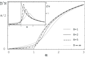
Figure 1: Numerical results for the scaled BP as a function of the parameter $\alpha$, for $D=10$ and for different values of $N$, in comparison with the result for $N\rightarrow\infty$. The BP increases with the coupling, and, in the thermodynamic limit, it displays a cusp at the critical value $\alpha=1$. The inset shows the derivative of the BP with respect to $\alpha$.

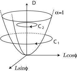
Figure 2: A qualitative illustration of the paths followed by the parameters of the Hamiltonian due to the application of $U(\phi)$. The paraboloid corresponds to the value $\alpha=L^{2}/2D=1$, for which the Hamiltonian shows a critical behavior. If the parameters follow a path, e.g. $C_{1}$, encircling the paraboloid, then the system acquires a non-trivial BP, which tends to $\pi$ for $\alpha\gg 1$. As seen from figure 1, path $C_{2}$ gives rise to a zero Berry phase (in the thermodynamical limit).

One can see that the BP increases with increasing the coupling strength and, in the thermodynamic limit, its derivative becomes discontinuous at the critical value $\alpha=\alpha_{c}=1$. This results are in accordance with the expected behavior of the BP across the critical point. Notice that, in the thermodynamic limit, a non-trivial Berry phase is only obtained when a region of criticality is encircled, as for the path $C_{1}$ in Fig. 2. Indeed, in the enlarged parameter space generated by the application of the unitary operator $U(\phi)$ of Eq. (2), the critical point corresponds to the paraboloid $\alpha=\frac{L^{2}}{2D}=1$. As the radius of the path is determined by $\alpha$, one can see that, in the limit $N\rightarrow\infty$, the BP is zero in the normal phase ($\alpha\leq 1$) and is non-zero in the super-radiant phase, i.e. if the path encloses the critical region.

We now investigate the scaling behavior of BP at the critical point by a finite size scaling approach. In order to obtain an analytic estimation of BP as a function of $N$, we expand the adiabatic potential in Eq.(12) and obtain an anharmonic oscillator potential

$$U_{l}(q)=\frac{2}{\omega}V_{l}(q)\simeq-ND+(1-\alpha)q^{2}+\frac{\alpha^{2}}{2ND}q^{4}$$ (19)

The eigenvalue problem defined by this potential can be solved with the help of Symanzik scaling finite ; simon . This is done by rewriting Eq.(12) into the equivalent form

$$\left[-\frac{d^{2}}{dx^{2}}+\zeta x^{2}+x^{4}\right]\varphi_{0}(x;\zeta)=e_{0}\left(\zeta\right)\varphi_{0}(x;\zeta)$$ (20)

where the scaled position is $x=q\left(\frac{\alpha^{2}}{2ND}\right)^{1/6}$, while $\zeta=\left(\frac{2ND}{\alpha^{2}}\right)^{2/3}(\alpha_{c}-\alpha)$. Finally, the energies in Eq.(12) and (20) obey the scaling relation

$$\frac{2}{\omega}\varepsilon_{0}(\alpha,ND)=-ND+\left(\frac{\alpha^{2}}{2ND}\right)^{1/3}e_{0}\left(\zeta\right).$$ (21)

Since $\zeta\rightarrow 0$ at the critical point, we can consider the $x^{2}$ term to be a perturbation and employ the Rayleigh-Schrödinger perturbation theory. This yields the expansion $e_{0}(\zeta)=\sum_{n=0}^{\infty}c_{n}\zeta^{n}$, where the coefficients $c_{n}$ can be obtained after solving the equation for a purely quartic oscillator. It is easy to get $c_{0}=e_{0}(0)\simeq 1.06036$ and $c_{1}=\int_{-\infty}^{\infty}q^{2}\phi_{0}^{2}(q;0)dq=e_{0}^{\prime}(0)\simeq 0.36203$.

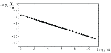
Figure 3: Scaling of the BP as a function of $N$ at the critical point $\alpha=1$, for $D=10$. For easy of comparison, the continuous plot shows the analytic expression of Eq. (23).

It can be shown that the coefficients of this expansion completely determine the average value of every physical observable at the critical point finite . In particular, a similar expansion applied to $\langle S_{x}\rangle$, allows us to write

$$\frac{\langle S_{x}\rangle}{N}\simeq-1+\frac{2c_{1}}{(2ND)^{2/3}}-\frac{2c_{0}}{(2ND)^{4/3}}.$$ (22)

Thus, we obtain the leading orders in the finite size scaling of the Berry phase as

$$\frac{\gamma}{N}\approx\pi\left[\frac{2c_{1}}{(2ND)^{2/3}}-\frac{2c_{0}}{(2ND)^{4/3}}\right].$$ (23)

This expression shows how the scaled geometric phase goes to zero as $N$ increases and how the singular thermodynamic behavior is approached at $\alpha=\alpha_{c}=1$. This analytical result, and in particular the leading critical behavior $\gamma/N\sim N^{-2/3}$ is confirmed in Fig. (3) by comparison with the BP obtained numerically from Eqs. (15)-(16). In fact, including also the second order correction scaling as $N^{-4/3}$, we are able to reproduce the numerical result even for small values of $N$.

Besides the scaling relation at the critical point $\alpha=1$, we can also obtain the leading $1/N$ correction to the thermodynamic limit of $\frac{\gamma}{N}$ for small and large values of $\alpha$. Using the fact that the oscillator localizes around $q=0$ for $\alpha\ll 1$, while its wave function is split in two components peaked around $\pm q_{m}$ for $\alpha\gg 1$, we get

$$\frac{\gamma}{N}-\frac{\gamma}{N}\Bigr{|}_{N\rightarrow\infty}\approx\left\{\begin{array}[]{ll}\hbox{$\frac{\pi\alpha}{2ND}$}&\hbox{$(\alpha\ll 1)$}\\ \hbox{$-\frac{\pi}{ND\alpha^{2}}$}&\hbox{$(\alpha\gg 1)$}\\ \end{array}\right.$$ (24)

To conclude, we have shown that the behavior of the geometric phase in correspondence of the critical region for the Dicke Model, confirms an expected connection between BP and QPT. Indeed, BP and QPT share the common feature of both appearing in presence of a singularity in the energy density of the system. This heuristic argument motivates the need to explore the use of BP as a tool to signal and investigate critical features of certain models. However, strictly speaking, singularities in the energy density of many body systems only appear in the thermodynamic limit. It is therefore not obvious that in a finite scale regime, such a connection between BP and QPT can still be drawn. Studying the BP in this regime has clearly theoretical interest and obvious experimental motivations. In the case of the Dicke model, we have found that the geometric phase shows, at finite sizes, a precursor of the topological character which appears in the thermodynamic limit. Moreover, studying the scaling of the BP as a function of the system size, we have identified its critical exponent.

References

- (1) M. V. Berry, Proc. R. Soc. A 392, 45 (1984).
- (2) H. C. Longuet-Higgins, U. Opik, M. H. L. Pryce, R. A. Sack, Proc. Roy. Soc. London Ser. A, 244,1, (1958).
- (3) G. Herzberg and H. C. Longuet-Higgins, Discuss. Faraday Soc., 35, 77 (1963).
- (4) A. Bohm, A. Mostafazadeh, H. Koizumi, Q. Niu, ad J. Zwanziger, The Geometric Phase in Quantum Systems. Springer-Verlag Berlin Heidelberg New York, 2003.
- (5) A. Shapere, and F. Wilczek (eds.), Geometric phases in physics. World Scientific, Singapore, 1989.
- (6) A. Carollo, J.K. Pachos, Phys Rev Lett, 95, 157203, (2005).
- (7) A. Hamma, preprint: quant-ph/0602091
- (8) Shi-Liang Zhu, Phys Rev Let, 96 077206, (2006).
- (9) S. Sachdev, Quantum Phase Transitions. Cambridge University press, 1999.
- (10) R.H. Dicke, Phys. Rev. 93, 99 (1954).
- (11) K. Hepp and E. Lieb, Ann. Phys. 76 (1973) 360; Phys. Rev. A 8 (1973) 2517.
- (12) Y.K. Wang and F.T. Hioe, Phys. Rev. A 7, 831 (1973).
- (13) G.C. Duncan, Phys. Rev. A 9, 418 (1974).
- (14) R. Gilmore and C.M. Bowden, Phys. Rev. A 13, 1898 (1976).
- (15) M. Orszag, J. Phys. A: Math. Gen. 10, L21 (1977).
- (16) S. Sivasubramanian, A. Widom and Y. Shrivastava, Physica A 301, 241 (2001)
- (17) G. Liberti and R.L. Zaffino, Phys. Rev. A 70, 033808 (2004); Eur. Phys. J. B 44, 535 (2005).
- (18) S. Schneider and G.J. Milburn, Phys. Rev. A 65, 042107 (2002).
- (19) C. Emary, T. Brandes, Phys. Rev. Lett. 90, 044101 (2003); Phys. Rev. E 67, 066203 (2003).
- (20) M. Frasca, Ann. Phys. 313, 26 (2004).
- (21) X. Hou and B. Hu, Phys. Rev. A 69, 042110 (2004).
- (22) V. Bužek, M. Orszag and M. Roško, Phys. Rev. Lett. 94, 163601 (2005).
- (23) T. Brandes, Phys. Rep. 408, 315 (2005).
- (24) N. Lambert, C. Emary and T. Brandes, Phys. Rev. Lett. 92, 073602 (2004); Phys. Rev. A 71, 053804 (2005).
- (25) J. Reslen, L. Quiroga and N.F. Johnson, Europhys. Lett. 69, 8 (2005).
- (26) J. Vidal and S. Dusuel, cond-mat/0510281.
- (27) G. Liberti et al., Phys. Rev. A 73, 032346 (2006).
- (28) G. Liberti, F. Plastina and F. Piperno, quant-ph/0603267.
- (29) B. Simon and A. Dicke, Ann. Phys. 58, 76 (1970).