Probability density function characterization of multipartite entanglement

Abstract

We propose a method to characterize and quantify multipartite entanglement for pure states. The method hinges upon the study of the probability density function of bipartite entanglement and is tested on an ensemble of qubits in a variety of situations. This characterization is also compared to several measures of multipartite entanglement.

I Introduction

Entanglement is one of the most intriguing features of quantum mechanics. Although it is widely used in quantum communication and information processing and plays a key role in quantum computation, it is not fully understood. It is deeply rooted into the linearity of quantum theory and in the superposition principle and basically consists (for pure states) in the impossibility of factorizing the state of the total system in terms of states of its constituents.

The quantification of entanglement is an open and challenging problem. It is possible to give a good definition of bipartite entanglement in terms of the von Neumann entropy and the entanglement of formation woot . The problem of defining multipartite entanglement is more difficult druss and no unique definition exists: different measures capture in general different aspects of the problem multipart . Attempts to quantify the degree of quantum entanglement are usually formulated in terms of its behavior under local operations/actions that can be performed on different (possibly remote) parts of the total system. Some recent work has focused on clarifying the dependence of entanglement on disorder and its interplay with chaos entvschaos ; SC , or its behavior across a phase transition QPT ; tognetti .

The work described here is motivated by the observation that as the size of the system increases, the number of measures (i.e. real numbers) needed to quantify multipartite entanglement grows exponentially. A good definition of multipartite entanglement should therefore hinge upon some statistical information about the system. We shall look at the distribution of the purity of a subsystem over all possible bipartitions of the total system. As a characterization of multipartite entanglement we will not take a single real number, but rather a whole function: the probability density of bipartite entanglement between two parts of the total system. The idea that complicated phenomena cannot be “summarized” in a single (or a few) number(s) stems from studies on complex systems parisi and has been considered also in the context of quantum entanglement MMSZ . In a few words, we expect that multipartite entanglement be large when bipartite entanglement is large and does not depend on the bipartition, namely when its probability density is a narrow function centered at a large value. This characterization of entanglement will be tested on several classes of states and will be compared with several measures of multipartite entanglement.

II The system

We shall focus on a collection of $n$ qubits. The dimension of the Hilbert space is $N=2^{n}$ and the two partitions $A$ and $B$ are made up of $n_{A}$ and $n_{B}$ spins ($n_{A}+n_{B}=n$), respectively, where the total Hilbert space reads $\mathcal{H}=\mathcal{H}_{A}\otimes\mathcal{H}_{B}$ and the Hilbert spaces $\mathcal{H}_{A}$ and $\mathcal{H}_{B}$ have dimensions $N_{A}=2^{n_{A}}$ and $N_{B}=2^{n_{B}}$, respectively ($N_{A}N_{B}=N$). We shall consider only pure states

$$|\psi\rangle=\sum_{k=0}^{N-1}z_{k}|k\rangle,$$ (1)

where $|k\rangle=|j_{A}\rangle\otimes|l_{B}\rangle$, with a bijection between $k$ and $(j_{A},l_{B})$, $0\leq j_{A}\leq N_{A}-1$ and $0\leq l_{B}\leq N_{B}-1$. As a measure of bipartite entanglement between $A$ and $B$ we consider the participation number

$$N_{AB}=\pi_{AB}^{-1},\quad\pi_{AB}=\mathop{\text{Tr}}\nolimits_{A}\rho_{A}^{2},\quad\rho_{A}=\mathop{\text{Tr}}\nolimits_{B}\rho,$$ (2)

where $\rho=|\psi\rangle\langle\psi|$, and $\mathop{\text{Tr}}\nolimits_{A}$ ($\mathop{\text{Tr}}\nolimits_{B}$) is the partial trace over the degrees of freedom of subsystem $A$ ($B$). $N_{AB}$ can be viewed as the relevant number of terms in the Schmidt decomposition of $|\psi\rangle$ eberly . The quantity $n_{AB}=\log_{2}N_{AB}$ represents the effective number of entangled spins. Clearly, for a completely separable state, $\mathop{\text{Tr}}\nolimits_{A}\rho_{A}^{2}=1$ for all possible bipartitions, yielding $N_{AB}=1$ and $n_{AB}=0$. In this sense the participation number can distinguish between entangled and separable states. Moreover $\pi_{AB}$ is directly related to the linear entropy $S_{L}=1-\pi_{AB}$, that is an entanglement monotone, i.e. it is non increasing under local operations linentropy and classical communication. In general, the quantity $N_{AB}$ will depend on the bipartition, as in general entanglement will be distributed in a different way among all possible bipartitions. Therefore, its distribution $p(N_{AB})$ will yield information about multipartite entanglement: its mean will be a measure of the amount of entanglement in the system, while its variance will measure how well such entanglement is distributed, a smaller variance corresponding to a higher insensitivity to the particular choice of the partition.

We will show that for a large class of pure states, statistically sampled over the unit sphere, $p(N_{AB})$ is very narrow and has a very weak dependence on the bipartition: thus entanglement is uniformly distributed among all possible bipartitions. Moreover, $p(N_{AB})$ will be centered at a large value. These are both signatures of a very high degree of multipartite entanglement.

By plugging (1) into (2) one gets

$$\pi_{AB}=\sum_{j,j^{\prime}=0}^{N_{A}-1}\,\sum_{l,l^{\prime}=0}^{N_{B}-1}z_{jl}\bar{z}_{j^{\prime}l}z_{j^{\prime}l^{\prime}}\bar{z}_{jl^{\prime}}.$$ (3)

We note that $\pi_{AB}=\mathop{\text{Tr}}\nolimits_{A}\rho_{A}^{2}=\mathop{\text{Tr}}\nolimits_{B}\rho_{B}^{2}$ and $1/N_{A}\leq\mathop{\text{Tr}}\nolimits_{A}\rho_{A}^{2}\leq 1$, with the minimum (maximum) value attained for a completely mixed (pure) state $\rho_{A}$. Therefore,

$$1\leq N_{AB}=N_{BA}\leq\min\{N_{A},N_{B}\}.$$ (4)

A larger value of $N_{AB}$ corresponds to a more entangled bipartition $(A,B)$, the maximum value being attainable for a balanced bipartition, i.e. when $n_{A}=[n/2]$ (and $n_{B}=[(n+1)/2]$), where $[x]$ is the integer part of the real $x$, that is the largest integer not exceeding $x$, and the maximum possible entanglement is $N_{AB}=N_{A}=2^{n_{A}}=\sqrt{N}$ ($=\sqrt{N/2}$) for an even (odd) number of qubits. As anticipated, as a characterization of multipartite entanglement we will consider the distribution of $N_{AB}$ over all possible balanced bipartitions.

III Measuring multipartite entanglement: some examples

Let us illustrate this approach on the simplest non-trivial situation, that of three entangled qubits. If the pure state is fully factorized, say

$$|\psi\rangle=|k\rangle$$ (5)

for a given $0\leq k\leq 7$, then the reduced density matrix $\rho_{A}$ of every qubit is a pure state, whence

$$p(N_{AB})=\delta_{N_{AB},1}:$$ (6)

there is no entanglement. On the other hand, for a maximally entangled state

$$|\psi\rangle=\frac{1}{\sqrt{2}}(|000_{2}\rangle+|111_{2}\rangle),$$ (7)

one gets a completely mixed state for every partition, namely $\rho_{A}=\mathrm{I}_{2}/2$ and thus

$$p(N_{AB})=\delta_{N_{AB},2},$$ (8)

with maximum average and zero variance: there is maximum multipartite entanglement, fully distributed among the three qubits. The above probability distributions should be compared with an intermediate case like

$$|\psi\rangle=\frac{1}{\sqrt{2}}(|000_{2}\rangle+|110_{2}\rangle),$$ (9)

where the first couple of qubits are maximally entangled (Bell state) while the third one is completely factorized. In such situation one gets $\rho_{1}=\rho_{2}=\mathrm{I}_{2}/2$, while $\rho_{3}=|1\rangle\langle 1|$, whence

$$p(N_{AB})=\delta_{N_{AB},1}/3+2\delta_{N_{AB},2}/3.$$ (10)

This simple application discloses the rationale behind the quantity $p(N_{AB})$ as a measure of multipartite entanglement.

When the system becomes larger, the natural extension is towards larger (balanced) bipartitions. We stress that, besides the comment that follows Eq. (4), the use of balanced bipartitions is simply motivated by the fact that, in the thermodynamical limit, the unbalanced ones give a small contribution, from the statistical point of view: this can be easily understood if one considers that for $n$ large and $n_{A}\ll n$ the binomial coefficients

$$\left(\begin{array}[]{c}n\\ n/2\\ \end{array}\right)\gg\left(\begin{array}[]{c}n\\ n_{A}\\ \end{array}\right),$$ (11)

so that our characterization of multipartite entanglement will be largely dominated by balanced bipartitions. Notice also that very unbalanced bipartitions of large systems yield negligible average entanglement kendon . For all these reasons, if one considers the distribution over all bipartitions, the contribution from the balanced bipartitions will dominate due to (11). By contrast, if only unbalanced bipartitions are considered the results will be in general very different.

It is interesting to study the features of the characterization of entanglement proposed in Sec. II when applied to particular classes of states. For the GHZ states ghz we find

$$N_{AB}(\text{GHZ})=2$$ (12)

for all possible bipartitions (both balanced and unbalanced) and for an arbitrary number of qubits. Clearly, the width of the distribution is 0, i.e. $p(N_{AB})=\delta_{N_{AB},2}$.

For the W states w we obtain

$$N_{AB}(\text{W})=\frac{n^{2}}{n_{A}^{2}+n_{B}^{2}}.$$ (13)

This value depends only on the relative size of the two partitions, i.e. also in this case the width of the distribution of bipartite entanglement is 0. Notice that, if $n$ is even, $N_{AB}(\text{W})=2$ for balanced bipartitions (and in this case a discrimination between W and GHZ states would require the analysis of unbalanced bipartitions). Moreover, in the large $n$ limit $N_{AB}(\text{W})\simeq 2$ also for $n$ odd.

These results indicate that, for $n$ large, the amount of (multipartite) entanglement is limited both for GHZ and W states. These states essentially share the same amount of entanglement when $n$ is large. They can be distinguished only by considering less relevant (from the statistical point of view) bipartitions. Moreover, for $n$ large, $N_{AB}(\text{W})\neq 1$ for balanced bipartitions. This means that also in the thermodynamical limit the W states retain some entanglement.

IV Typical states

Let us now study the typical form of our characterization of multipartite entanglement $p(N_{AB})$ for a very large class of pure states of the form (1), sampled according to a given statistical law. Several features of these random states are already known in the literature SC ; aaa ; EH , but we shall focus on those quantities that are relevant for our purpose. We write

$$|\psi\rangle=\sum_{k=0}^{N-1}r_{k}e^{i\phi_{k}}|k\rangle,$$ (14)

where $\phi_{k}$ are independent random variables with expectation

$$E[e^{i\phi_{k}}]=0$$ (15)

and ${\bm{r}}=(r_{1},\dots,r_{N})$ is a random point with a given symmetric distribution $p(\bm{r})$ on the hypersphere $S^{N-1}=\{{\bm{r}}\in\mathbb{R}^{N}|{\bm{r}}^{2}=1\}$. The features of these random states are readily evaluated: one first splits $\pi_{AB}$ in two parts

$$\pi_{AB}=X_{AB}+M_{AB},$$ (16)

where

$$X_{AB} = {\sum_{j,j^{\prime}}}^{\prime}{\sum_{l,l^{\prime}}}^{\prime}r_{jl}r_{j^{\prime}l}r_{j^{\prime}l^{\prime}}r_{jl^{\prime}}e^{i(\phi_{jl}-\phi_{j^{\prime}l}+\phi_{j^{\prime}l^{\prime}}-\phi_{jl^{\prime}})},$$

$$M_{AB} = {\sum_{j,j^{\prime}}}^{\prime}{\sum_{l}}r_{jl}^{2}r_{j^{\prime}l}^{2}+\sum_{j}{\sum_{l,l^{\prime}}}^{\prime}r_{jl}^{2}r_{jl^{\prime}}^{2}+\sum_{j,l}r_{jl}^{4},$$ (18)

with $j,j^{\prime}=0,\dots,N_{A}-1$, $l,l^{\prime}=0,\dots,N_{B}-1$, and primes banning equal indices in the sums.

We note that the expectation value $E[r_{jl}^{2}]=O(1/N)$, thus $X_{AB}$ and $M_{AB}$ are sums of at most $N^{2}$ terms of order $1/N^{2}$. By the central limit theorem, for large $N$, $\pi_{AB}$ tends to a Gaussian random variable with mean and variance

$$\mu_{AB} = E[\pi_{AB}],$$

$$\sigma^{2}_{AB} = E[\pi_{AB}^{2}]-\mu_{AB}^{2},$$ (19)

respectively, namely it is distributed as

$$f(\pi_{AB})=\frac{1}{(2\pi\sigma_{AB}^{2})^{\frac{1}{2}}}\exp\left(-\frac{(\pi_{AB}-\mu_{AB})^{2}}{2\sigma_{AB}^{2}}\right).$$ (20)

From $E[X_{AB}]=0$ and the independence between phases $\phi_{k}$ and moduli $r_{k}$ we get

$$\mu_{AB}=E[M_{AB}]=N(N_{A}+N_{B}-2)E[r_{1}^{2}r_{2}^{2}]+NE[r_{1}^{4}]$$ (21)

and

$$\sigma^{2}_{AB}=E[X^{2}_{AB}]+E[M^{2}_{AB}]-\mu^{2}_{AB},$$ (22)

where

$$E[X^{2}_{AB}]=2N(N_{A}-1)(N_{B}-1)E[r_{1}^{2}r_{2}^{2}r_{3}^{2}r_{4}^{2}]$$ (23)

and

$$E[M^{2}_{AB}]=N(N_{A}+N_{B}-2)$$

$$\qquad\quad\times[(N_{A}+N_{B})(N-4)-2(N-5)]E[r_{1}^{2}r_{2}^{2}r_{3}^{2}r_{4}^{2}]$$

$$+2N(N_{A}+N_{B}-2)(N+2N_{A}+2N_{B}-8)E[r_{1}^{2}r_{2}^{2}r_{3}^{4}]$$

$$+N(N+2N_{A}+2N_{B}-5)E[r_{1}^{4}r_{2}^{4}]$$

$$+4N(N_{A}+N_{B}-2)E[r_{1}^{2}r_{2}^{6}]+NE[r_{1}^{8}],$$ (24)

where we used $E[r_{1}^{\alpha}r_{2}^{\beta}r_{3}^{\gamma}r_{4}^{\delta}]=E[r_{i}^{\alpha}r_{j}^{\beta}r_{l}^{\gamma}r_{k}^{\delta}]$ with $i,j,l,k$ all distinct. Notice that the above results do not depend on the particular distribution of $\phi_{k}$, as far as the condition (15) is satisfied (otherwise the analysis is still valid, but Eqs. (21)-(24) become more involved). Our results particularize for the case of a typical pure state (1), sampled according to the unitarily invariant Haar measure, where each $z_{k}\in\mathbb{C}$ is chosen from an ensemble that is uniformly distributed over the projective Hilbert space $\sum_{k}|z_{k}|^{2}=1$. In such a case, in (14), $\phi_{k}\in[0,2\pi]$ are independent uniformly distributed random variables and ${\bm{r}}=(r_{1},\dots,r_{N})$ is a random point uniformly distributed on the hypersphere $S^{N-1}$, with distribution function

$$p(\bm{r})=\frac{2^{N}}{\pi^{N/2}}\,\Gamma\left(\frac{N}{2}\right)\delta(1-\bm{r}^{2}),$$ (25)

the prefactor being twice the inverse area of the hyperoctant $\{r_{i}>0\}$, with $\Gamma(x)$ the Gamma function.

The explicit expressions of (21)-(24) can be computed through (25), recovering the values of mean and variance obtained by different approaches aaa ; SC ; EH . However one can easily estimate them for large $N$ by the following reasoning. For large $N$ the marginal distributions of the amplitudes $r_{k}$ become normal,

$$p(r_{k}) = \frac{2}{\sqrt{\pi}}\frac{\Gamma(N/2)}{\Gamma\left((N-1)/2\right)}{\left(1-r_{k}^{2}\right)}^{(N-3)/2}$$ (26)

$$\sim 2\sqrt{\frac{N}{2\pi}}\exp\left(-\frac{N}{2}r_{k}^{2}\right)\qquad(\forall k),$$

with variance $1/N$. One can convince oneself of the correctness of the above expression just by recalling the asymptotic behavior of gamma function and expanding $(1-r_{k}^{2})^{N/2}$. Moreover it is not difficult to show that the $r_{k}$’s become uncorrelated, hence independent. Therefore the expectation of products factorizes and $E[r_{1}^{2m}]=(2m-1)!!/N^{m}$, yielding

$$\mu_{AB}=\frac{N_{A}+N_{B}-1}{N},\quad\sigma^{2}_{AB}=\frac{2}{N^{2}}.$$ (27)

It is important to notice that when $N\gg 1$ we can effectively replace $r_{k}$ with its mean square root value, $r_{k}=1/\sqrt{N}$, from which (27) immediately follows. In the simulation plotted in Fig. 1 we used the above substitution. The fact that for Haar distributed states the average (27) is concentrated around a large value was already recognized by other authors aaa ; SC ; EH .

$n$	GHZ	W	cluster	random
5	2	1.923	3.6	2.909
6	2	2	5.4	4.267
7	2	1.96	6.171	5.565
8	2	2	8.743	8.258
9	2	1.976	10.349	10.894
10	2	2	14.206	16.254
11	2	1.984	17.176	21.558
12	2	2	23.156	32.252

Table 1: Mean bipartite entanglement $E[N_{AB}]$, analitically evaluated according to Eqs. (12), (13) and (27). The values for the cluster state were computed by inserting (29) in the definitions (2)-(3).

The quantity of interest is $N_{AB}$ defined in Eq. (2). From Eq. (20), its probability density reads

$$p(N_{AB}) = \frac{1}{N^{2}_{AB}(2\pi\sigma_{AB}^{2})^{1/2}}\exp\left(-\frac{(N_{AB}^{-1}-\mu_{AB})^{2}}{2\sigma_{AB}^{2}}\right).$$

It is interesting to compare the features of the random states with those of other states studied in the literature. Table 1 displays the average value of $N_{AB}$ (evaluated for $n=5\div 12$) for GHZ states ghz , W states w , the generic states (14) and one-dimensional cluster states briegel defined as

$$|\phi_{n}\rangle=\frac{1}{\sqrt{2^{n}}}\bigotimes_{k=1}^{n}(|0\rangle_{k}\sigma^{(k+1)}_{z}+|1\rangle_{k}),$$ (29)

where $\sigma_{z}$ is the third Pauli matrix and the convention $\sigma^{(n+1)}_{z}=1$ is applied. While the entanglement of the GHZ and W states is essentially independent of $n$ [see Eqs. (12)-(13)], the situation is drastically different for cluster and random states. In both cases, the average entanglement increases with $n$; for $n>8$ the average entanglement is higher for random states. However, it is now clear that the average $E[N_{AB}]$ yields poor information on multipartite entanglement. For this reason, it is useful to analyze the distribution of bipartite entanglement over all possible balanced bipartitions. The results for the cluster and random states are shown in Fig. 1, for $n=5\div 12$, where the product of the probability density $p$ times the number of bipartitions $n_{p}=n!/n_{A}!n_{B}!$ is plotted vs $N_{AB}$. Notice that the distribution function of the random state is always peaked around $\mu_{AB}^{-1}$ in (27) and becomes narrower for larger $n$, in agreement with $\sigma^{2}_{AB}$ in (27). Notice also that the cluster state can reach higher values of $N_{AB}$ (the maximum possible value being $2^{[n/2]}$), however, the fraction of bipartitions giving this result becomes smaller for higher $n$. This is immediately understood if one realizes that cluster states are designed for optimized applications and therefore perform better in terms of specific bipartitions. On the other hand, according to the characterization we propose, the random states (14) are characterized by a large value of multipartite entanglement, that is roughly independent on the bipartition. The probability density functions (LABEL:eq:distrpartnumber) are displayed in Fig. 2.

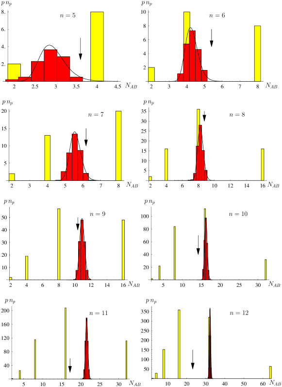
Figure 1: Number of balanced bipartitions vs $N_{AB}$; $p$ is the probability density, $n_{p}=n!/n_{A}!n_{B}!$ is the number of bipartitions. The yellow bars represent one-dimensional cluster states [see Eq. (29)], the red ones random states; the solid line is the distribution (27)-(LABEL:eq:distrpartnumber); the black arrows indicate the average $\langle N_{AB}\rangle_{\text{cluster}}$. For even $n$ ($n=12$ in particular) the distribution of the random state partially hides a peak of the corresponding cluster state distribution, centered at $N_{AB}=2^{n_{A}-1}=2^{[n/2]-1}$.

Figure 2: Probability densities functions (LABEL:eq:distrpartnumber) vs $N_{AB}$. Each curve is labeled with the corresponding value of $n$ (number of qubits). The standard deviation of the distribution is essentially independent of $n$.

A few additional comments on random states are in order. In the thermodynamical limit

$$\frac{\sigma_{AB}}{\mu_{AB}}=\frac{\sqrt{2}}{N_{A}+N_{B}-1}=O(1/\sqrt{N})$$ (30)

and the single real number $E[N_{AB}]$ is sufficient to characterize multipartite entanglement (modulo more accurate thermodynamical considerations).

In general, for finite systems, the mean bipartite entanglement $N_{AB}\simeq\mu_{AB}^{-1}$ in (27) is maximum for $N_{A}=N_{B}=\sqrt{N}$ ($N_{A}=N_{B}/2=\sqrt{N/2}$) for even (odd) $n$, namely for balanced bipartitions. Notice however that, as we already emphasized a number of times in this article, although we focused on balanced bipartitions for illustrative purposes, the main results are valid when one includes also unbalanced bipartitions, as, by virtue of (11), the contribution of the balanced bipartition will be exponentially dominant.

Moreover, for large $N$, any (symmetric) radial distribution $p(\bm{r})$ yields the same results (27), the only relevant feature being the curvature in the projective Hilbert space, forced by the normalization $\bm{r}^{2}=1$ [see for example (25)]. In this sense, the above analysis is of general validity, being independent of the particular choice of the ensemble.

V Comparison with some multipartite entanglement measures

It is interesting to compare our proposed characterization of multipartite entanglement with some other entanglement measures. In general, we will find that this characterization sheds additional light on this issue and helps specify some of the global features of multipartite entanglement in a clear-cut way.

The quantity brennen

$$Q(|\psi\rangle)=2\left(1-\frac{1}{n}\sum_{k}\mathrm{Tr}{\rho^{2}_{\{k\}}}\right),$$ (31)

where $\rho_{\{k\}}$ is the reduced density matrix of qubit $k$, i.e. $\rho_{A}$ with $A=\{k\}$. In our language, it corresponds to the mean value of $\pi_{AB}$ over maximally unbalanced bipartitions, namely

$$Q(|\psi\rangle)=2\left(1-E_{\text{max unbal}}[\pi_{AB}]\right).$$ (32)

For W states this yields $Q(\text{W})\sim 0$ for large $n$. This should be compared with the value $N_{AB}(W)=2$ (exact for even $n$, approximate for odd $n$), obtained by considering balanced bipartitions of the system. As previously stressed, this means that the W states retain some entanglement even in the thermodynamical limit.

Moreover, at variance with $Q$, the mean value of $N_{AB}$ can distinguish sub-global entanglement. For instance, the state $|\psi\rangle=(|0\rangle|0\rangle+|1\rangle|1\rangle)\otimes(|0\rangle|0\rangle+|1\rangle|1\rangle)/2$ cannot be distinguished from the GHZ state by using only $Q$. On the other hand, one gets an average $\langle N_{AB}\rangle=3$ and a width for the distribution $\sigma=1.55$. Another interesting point is that the distribution of $N_{AB}$ can distinguish GHZ and cluster states (actually the average is already sufficient, as can be seen from Table 1). From these results one can argue that the probability density function of the participation number $N_{AB}$ not only better specifies the meaning of $Q$ but also yields additional information.

It is also interesting to recall the behavior of the pairwise entanglement (concurrence) and the tangle multipart . The former is defined (for states $\rho_{\{i,j\}}$ of two qubits $i$ and $j$) as

$$C_{ij}=\mbox{max}(0,\lambda_{1}-\lambda_{2}-\lambda_{3}-\lambda_{4}),$$ (33)

where $\lambda_{k}$ are the square roots of the eigenvalues (in decreasing order) of the matrix $\rho_{\{i,j\}}\sigma_{y}\otimes\sigma_{y}\rho^{*}_{\{i,j\}}\sigma_{y}\otimes\sigma_{y}$, and is therefore related to $\pi_{AB}$ with $A=\{i,j\}$ (highly unbalanced bipartitions when $N$ is large). The tangle is defined as

$$\tau_{1}^{(i)}=4\det\rho_{\{i\}}=2(1-\mathrm{Tr}{\rho^{2}_{\{i\}}}),$$ (34)

where $\rho_{\{i\}}$ is the reduced density matrix for qubit $i$. Note that $\tau_{1}^{(i)}=2(1-\pi_{AB})$, with $A=\{i\}$, is nothing but the local version of $Q$ in (31). In particular one can consider the ratio $R^{(i)}=\tau_{2}^{(i)}/\tau_{1}^{(i)}$ tognetti where $\tau_{2}^{(i)}=\sum_{j\neq i}C_{ij}^{2}$ is the sum of the squared concurrences of qubit $i$ with qubit $j$. Due to the Coffman-Kundu-Wootters conjecture $\tau_{1}^{(i)}\geq\tau_{2}^{(i)}$ multipart one can take $R^{(i)}$ as a witness of multipartite entanglement: if $R^{(i)}<1$ pairwise entanglement is less relevant than multi-qubit correlations. In particular, in order to elucidate their relation with the bipartite entanglement of highly unbalanced bipartitions, it is interesting to apply these measures to typical states. We notice that, in the limit of large $n$ one has, on the average,

$$E[\tau_{1}] = Q=1-1/2^{n-1}\sim 1,$$

$$E[\tau_{2}] \sim 0.$$ (35)

These results are interesting because they show how, in the thermodynamical limit, pairwise entanglement is negligible for typical states. At the same time, Eq. (V) does not yield much information about the very structure of multipartite entanglement: actually one can see that the same result can be obtained for GHZ states (for arbitrary $n$). In this sense our characterization in terms of the probability density function corroborates and better specifies the results obtained by studying the behavior of $R$.

VI Conclusions

It is well known that an efficient way to generate states endowed with random features is by a chaotic dynamics entvschaos ; SC , or at the onset of a quantum phase transition QPT . In particular, the random states (14) describe quite well states with support on chaotic regions of phase space, before dynamical localization has taken place. Interestingly, other ways have been recently proposed EH ; plenio in order to generate these states, in particular by operating on couples of qubits with random unitaries followed by CNOT gates plenio . The introduction of a probability density function as a measure of multipartite entanglement paves the way to further investigations of this intimate relation between entanglement and randomness. Work is in progress in order to clarify whether the random states can be efficiently used in quantum information processing.

In some sense, the characterization we propose quantifies the robustness of entanglement against all possible partial tracing. Clearly, it is more effective for large number of qubits and when relatively few moments are sufficient to specify the distribution. We stress that although we studied the distribution function of the inverse purity (linear entropy) (2), our analysis could have been performed in terms of any other measure of bipartite entanglement, such as the entropy.

Finally, we emphasize again the main motivation behind this work: as the number of subsystems increases, the number of measures (i.e. real numbers) needed to quantify multipartite entanglement grows exponentially. It is therefore not surprising if a satisfactory global characterization of entanglement requires the use of a function.

- (1) W. K. Wootters, “Quantum Information and Computation” (Rinton Press, 2001), Vol. 1; C. H. Bennett, D. P. DiVincenzo, J. A. Smolin, and W. K. Wootters, Phys. Rev. A 54, 3824 (1996).
- (2) D. Bruss, J. Math. Phys. 43, 4237 (2002).
- (3) V. Coffman, J. Kundu and W. K. Wootters, Phys. Rev. A 61, 052306 (2000); A. Wong and N. Christensen, Phys. Rev. A 63, 044301 (2001); D.A. Meyer and N.R. Wallach, J. Math. Phys. 43, 4273 (2002).
- (4) J. N. Bandyopadhyay and A. Lakshminarayan Phys. Rev. Lett. 89 060402 (2002); S. Montangero, G. Benenti, and R. Fazio, Phys. Rev. Lett. 91, 187901 (2003); S. Bettelli and D. L. Shepelyansky, Phys. Rev. A 67, 054303 (2003); A. J. Scott and C. M. Caves, J. Phys. A 36, 9553 (2003); L. F. Santos, G. Rigolin, and C. O. Escobar, Phys. Rev. A 69, 042304 (2004); N. Lambert, C. Emary, and T. Brandes, Phys. Rev. Lett. 92, 073602 (2004); C. Mej a-Monasterio, G. Benenti, G. G. Carlo, and G. Casati, Phys. Rev. A 71, 062324 (2005).
- (5) A. J. Scott and C. M. Caves, J. Math. Phys. 36, 9553 (2003).
- (6) A. Osterloh, L. Amico, G. Falci, and R. Fazio, Nature 416, 609 (2002); T. J. Osborne and M. A. Nielsen, Phys. Rev. A 66, 032110 (2002); I. Bose and E. Chattopadhyay, Phys. Rev. A 66, 062320 (2002); G. Vidal, J. I. Latorre, E. Rico, and A. Kitaev, Phys. Rev. Lett. 90, 227902 (2003); U. Glaser, H. Büttner, and H. Fehske, Phys. Rev. A 68, 032318 (2003); S. J. Gu, H. Q. Lin, and Y. Q. Li, Phys. Rev. A 68, 042330 (2003); L. Amico, A. Osterloh, F. Plastina, R. Fazio, and G. M. Palma, Phys. Rev. A 69, 022304 (2004); V. E. Korepin, Phys. Rev. Lett. 92, 096402 (2004); J. Vidal, G. Palacios, and R. Mosseri, Phys. Rev. A 69, 022107 (2004); F. Verstraete, M. Popp, and J. I. Cirac, Phys. Rev. Lett. 92, 027901 (2004).
- (7) T. Roscilde, P. Verrucchi, A. Fubini, S. Haas and V. Tognetti, Phys. Rev. Lett. 93, 167203 (2004); Phys. Rev. Lett. 94, 147208 (2005).
- (8) G. Parisi, “Statistical Field Theory” (Addison-Wesley, New York, 1988).
- (9) V. I. Man’ko, G. Marmo, E. C. G. Sudarshan and F. Zaccaria, J. Phys. A: Math. Gen. 35, 7137 (2002).
- (10) R. Grobe, K. Rza̧żewski and J.H. Eberly, J. Phys. B 27, L503 (1994); J.H. Eberly, “Schmidt Analysis of Pure-State Entanglement” quant-ph/0508019.
- (11) C. Emary, J. Phys. A 37, 8293 (2004); A. J. Scott, Phys. Rev. A 69, 052330 (2004).
- (12) V.M. Kendon, K. Życzkowski and W.J. Munro, Phys. Rev. A 66, 062310 (2002).
- (13) D.M. Greenberger, M. Horne and A. Zeilinger, Am. J. Phys. 58, 1131 (1990).
- (14) W. Dür, G. Vidal and J.I. Cirac, Phys. Rev. A 62, 062314 (2000).
- (15) K. Brennen, Quantum Inform. Comput. 3, 619 (2003).
- (16) E. Lubkin, J. Math. Phys. 19, 1028 (1978); S. Lloyd and H. Pagels, Ann. Phys., NY, 188, 186 (1988); K Życzkowski and H.-J. Sommers J. Phys. A 34, 7111 (2001); Y. Shimoni, D. Shapira and O. Biham, Phys. Rev. A 69, 062303 (2004).
- (17) J. Emerson, Y.S. Weinstein, M. Saraceno, S. Lloyd and DG Cory, Science 302, 2098 (2003); P. Hayden, D. W. Leung and A. Winter, Comm. Math. Phys., 265, 95-117, (2006).
- (18) H.J. Briegel and R. Raussendorf, Phys. Rev. Lett. 86, 910 (2001).
- (19) R. Olivera, O. Dahlsten and M.B. Plenio, quant-ph/0605126